Is Anonymization Through Discretization Reliable? Modeling Latent Probability Distributions for Ordinal Data as a Solution to the Small Sample Size Problem

Abstract

The growing interest in data privacy and anonymization presents challenges, as traditional methods such as ordinal discretization often result in information loss by coarsening metric data. Current research suggests that modeling the latent distributions of ordinal classes can reduce the effectiveness of anonymization and increase traceability. In fact, combining probability distributions with a small training sample can effectively infer true metric values from discrete information, depending on the model and data complexity. Our method uses metric values and ordinal classes to model latent normal distributions for each discrete class. This approach, applied with both linear and Bayesian linear regression, aims to enhance supervised learning models. Evaluated with synthetic datasets and real-world datasets from UCI and Kaggle, our method shows improved mean point estimation and narrower prediction intervals compared to the baseline. With 5–10% training data randomly split from each dataset population, it achieves an average 10% reduction in MSE and a ~5–10% increase in R² on out-of-sample test data overall.

1. Introduction

Today, both private and business data are incredibly valuable and are targeted by various interest groups at every possible junction. As a result, data privacy has become a highly relevant issue affecting both individuals and organizations. Often, however, data are handled carelessly, with an overreliance on existing anonymization methods, leading to potential risks.

The permanent recording and insufficiently regulated sale of anonymized data present significant risks of re-identification [1], which, according to current research, cannot be completely ruled out despite protective measures [2]. Experts in data governance warn against the false sense of security provided by data anonymization. Advanced machine learning models and statistical techniques, such as modeling probability distributions, are increasingly uncovering methods to re-identify supposedly anonymized data, thereby compromising anonymity [3].

Common challenges in this field include the small sample size problem, whereby the sample size has a significant impact on the generalizability of research findings [4]. According to common recommendations, it should not be less than 10% in pilot studies [5]. Additionally, computational complexity and the reliability of model predictions pose hurdles, as the forecasts depend on the reliability of the given data [6] and the quantification of uncertainties in the predictions [7].

This paper addresses the traceability and reversibility of anonymized metric data or target values through discretization, which may lead to security or information loss. Techniques such as ordinalization [8] and rounding [9] coarsen the metric space into adjacent ordinal classes, leading to information loss depending on the number of ordinal classes. Previous research has explored the evaluation of data based on discrete classes, considering the uncertainty of data [10], the optimum between data usability and maximum anonymity [11], and data diversity and characteristic details [12]. It has also investigated applying k-anonymization for de-identification [13], the conversion of ordinal classes back to metric values, focusing on assumptions about underlying distributions [14], and an unsupervised learning approach combined with discriminative information [15]. Other approaches have examined how rough set theory, as an example, benefits from discretizing continuous value ranges [16], the conditions under which it makes sense to convert the data [17], and how ordinal classes can be treated as a continuous space [18].

Recent studies have also shown improved methods for enhancing data privacy and anonymity [19,20,21,22,23,24,25], where the main focus is on providing a systematic overview of existing anonymization techniques, especially in light of the increasing availability of data from social networks [19], as well as a comparative study of five current techniques for anonymizing collected data, assessing their strengths and weaknesses [20]. Further research has reviewed existing methods such as generalization and bucketization [21], compared suppression with slicing with other common techniques [22], highlighted weaknesses related to the compatibility of independently generalized data [23], and explored anonymization through pseudonymization [24] and a pseudo creation technique [25]. Furthermore, it is interesting to note how the use of latent influencing factors based on ordinal classes improves Bayesian analysis [26] and generates more accurate classifications compared to traditional classification methods [27].

Modeling probabilistic distributions for latent categorical variables suggests that assuming a continuous latent distribution within ordinal classes allows for precise value derivation from limited data using machine learning models. This implies that probability distributions for ordinal classes, even with small datasets, can provide a good distributional model and a reliable approximation of the underlying continuous latent distribution. This paper aims to demonstrate that data coarsening for anonymization can be misleading and not fully reliable. We propose a new approach that enables high prediction accuracy of true metrics values from anonymized data using deterministic or probabilistic supervised learning regression models. The re-anonymized results are also analyzed for uncertainties.

In the following sections, we apply our approach to simulation studies on both low- and high-complexity synthetic data and conduct a benchmarking study with publicly available datasets from various application domains.

2. De-Anonymization of Metric Data

To ensure anonymity in surveys or, in general, in data protection, data discretization is an often-applied approach. This approach involves dividing metric or continuous data into classes, thereby coarsening it into discrete information. In this section, we describe our novel methodology for reliably reverting anonymized information to its true (metric) values, highlighting the issues of this anonymization technique.

2.1. Introduction to the Method

Our methodology is based on the assumption that even a small set of precise, non-discretized information (a very small training dataset with metric values) is sufficient to train models that are capable of de-anonymizing coarsened data and inferring the metric values of out-of-sample data, considering uncertainties. In the process, we model latent distributions (of each class) with normal distributions based on the available precise information and use these to generate probabilities for the discretized observations. The goal is to retrospectively reverse the discretization with minimal bias.

2.2. Process of Discretization

The new approach promises that reliable inferences for the entire discrete ordinal class can be drawn from just a few metric data points per class and their distributions. This logic describes the partitioning of the distribution of the entire metric space into ordered, discrete classes, each associated with a specific sampling distribution. Consequently, the division and choice of class boundaries significantly influence the sampling distribution within each class.

The grouping of data inevitably leads to a loss of information. However, statistical clustering methods that minimize squared errors can assist in optimally establishing group boundaries, thereby facilitating an optimal classification of normally distributed data concerning the frequency distribution within the class [28]. Other methodologies aim to reduce the complexity of continuous distributions while preserving as much information as possible through Representative Points (RPs). RPs can be generated using techniques such as Monte Carlo sampling, deterministic point selection, or MSE-based clustering, thereby optimizing classification by minimizing a loss function. The commonly used k-means algorithm can also be employed as an approach in this context [29].

In contrast to statistical grouping, there is also the possibility of a predefined, data-independent, or random classification into ordered classes. In practical applications, it may occur that existing classes are utilized by the methodology. Therefore, the objective of this paper is to model existing classes and boundaries that may contradict an optimal statistical clustering.

2.3. Theoretical Formulation

Let $X=\{x_1,x_2,x_3,\dots x_m\}$ be the feature matrix of $m$ independent variables, where each variable is assumed to be independently and identically distributed (i.i.d.). Let $y$ be the dependent target variable with the value range $W_y$. We address a regression problem

$$\begin{gathered} f:{\mathbb{R}}^{\mathrm{m}}\to W\subseteq \mathbb{R} \\ f:X\to y \end{gathered}$$

with a very small training sample relative to the test data (i.e., small sample size problem). We sloppily define the grid with $K+2$ subclasses as

$$grid\mid y=\{{class}_0,clas{s}_1,clas{s}_2,\dots ,clas{s}_K,{class}_{K+1}\mid y\}, \left|grid\right|=K+2$$

comprising disjoint ordinal classes that depend on the target variable $y$. The $grid$ refers to a finite set of ordered, ordinally scaled classes $\{0,1,2,\dots ,K+1\}$. Consequently, the following holds:

$$\{{class}_0,clas{s}_1,clas{s}_2,\dots ,clas{s}_{K+1}\}=\{0,1,2,\dots ,K,K+1\}.$$

Each class $k$ from the set $\{0,1,2,\dots ,K+1\}$ is defined by two threshold values, $a_k$ and $a_{k+1}$. These thresholds satisfy the following conditions:

$$-\mathrm{\infty }=a_0<a_1<\dots <a_K<a_{K+1}<a_{K+2}=\mathrm{\infty }.$$

As a result, the following holds:

$${\forall }_{k=1}^{K+1}{\forall }_{i=1}^n:y_i\in clas{s}_k\to y_i\in \left[a_k,a_{k+1}\right]\to a_k\le y_i<a_{k+1}$$

and for $k=0$:

$${\forall }_{i=1}^n:y_i\in clas{s}_0\to y_i\in \left[a_0,a_1\right]\to -\mathrm{\infty }=a_0<y_i<a_1.$$

$K+2$ classes are defined by $K+3$ thresholds. Hence, each class has a lower threshold $a_k$ and an upper threshold $a_{k+1}$, which partition the continuous value range $W$ of $y$ into discrete, adjacent subgroups. Specifically, this can be expressed as:

$$grid|y=\left[a_0,a_1,\dots ,a_K,a_{K+1},a_{K+2}\right]\subseteq W.$$

In the following application, we focus on a selected finite subset of the classes and their associated thresholds. Consequently, we disregard the outer classes $clas{s}_o=\left[a_0,a_1\right]$ and $clas{s}_{K+1}=\left[a_{K+1},a_{K+2}\right]$. This restriction does not impact the results because:

$${\forall }_{i=1}^n:y_i\in \left[a_1,\dots ,a_{K+1}\right]\subseteq \left[a_0,a_1,\dots ,a_K,a_{K+1},a_{K+2}\right]\subseteq W.$$

In the transformation $T$, the metric values $y$ are mapped to classes based on these thresholds:

$$\begin{gathered} T:\mathrm{W}\subseteq \mathbb{R}\to \left\{clas{s}_1,clas{s}_2,\dots ,clas{s}_{\mathrm{K}}\right\}\subseteq {\mathbb{N}}_0 \\ T:y\to \{1,\dots ,K\} \end{gathered}$$

The resulting vector $clas{s}^y$ is defined as a new, optionally applicable feature $X_{m+1}$, which is subsequently used as an ordinal-scaled variable and one-hot encoded.

Following, each class for each observation represents a discretized continuous value $y$. Now, we split the given data with observations $\{1,\dots ,n\}$ into training data $\{1,\dots ,l\}$ and test data $\left\{l+1,\dots ,n\right\}$. For each $k$-th ordinal class $clas{s}_k$, a normal distribution $N({\mu }_k,{\sigma }_k^2)$ is fitted by estimating its parameters using the mean and standard deviation formulas to approximate the histogram of the training data for $y\in clas{s}_k$. With mean ${\mu }_k$ and standard deviation ${\sigma }_k$ of the normal distribution for the $k$-th class from $k=\{1,\dots ,K\}$, it follows that:

$$\left({\forall }_{i=1}^l:y_i^{train}\in clas{s}_k\right)|clas{s}_k~N({\mu }_k,{\sigma }_k^2).$$

The parametric modeling of the normal distributions allows for determining the parameters $\mu$ and $\sigma$ for each class, and thus, the densities for each observation can be calculated. While random sampling from the distribution could be used to capture the properties of the density function as an input feature, we aim to provide more precise information for each observation. Therefore, we determine the absolute $f_i$ and relative frequency $p_i$ of $y_i$ based on the density of its class. For each $k$-th class, we determine the mean and standard deviation as follows:

$${\forall }_{k=1}^K:\mu \left(y\in clas{s}_k\right)={\mu }_k\wedge \sigma \left(y\in clas{s}_k\right)={\sigma }_k.$$

Then, we calculate the probability density function (PDF) value for the given train data $y_i^{train}$ given the $k$-th class:

$$f\left(y_i^{train}|clas{s}_k\right)={\displaystyle \frac{1}{{\sigma }_k\sqrt{2\pi }}}exp\left(-{\displaystyle \frac{{\left(y_i^{train}-{\mu }_k\right)}^2}{2{\sigma }_k^2}}\right)=f_{ik}$$

The PDF indicates how densely the random variable $y_i^{train}$ is distributed around a specific value. For the relative frequency density, we have:

$$p_{ik}^{train}={\displaystyle \frac{f_{ik}^{train}}{N_k^{train}}}$$

where $N_k^{train}$ is the total number of training samples in class $k$, and:

$$\sum _{k=1}^K{N}_k=\sum _{k=1}^K{N}_k^{train}+\sum _{k=1}^K{N}_k^{test}=\sum _{k=1}^K(N_k^{train}+N_k^{test})=n.$$

The relative frequency $p_{ik}^{train}$ thus provides a value that is proportional to the probability density at $y_i$, indicating how likely it is that $y_i$ lies in a small interval around the given point. By integrating the density over a continuous range

$$\left[b-{\displaystyle \frac{ϵ}{2}},b+{\displaystyle \frac{ϵ}{2}}\right]$$

with a sufficient small $ϵ$, the actual probability can be approximated by:

$$P\left(b-{\displaystyle \frac{ϵ}{2}}\le y_i\le b+{\displaystyle \frac{ϵ}{2}}|clas{s}_k\right)={\int }_{b-{\displaystyle \frac{ϵ}{2}}}^{b+{\displaystyle \frac{ϵ}{2}}}f\left(y_i|clas{s}_k\right)dy.$$

Since $f\left(y_i|clas{s}_k\right)$ is nearly constant within a sufficiently small interval around $b$, it follows that:

$$P\left(b-{\displaystyle \frac{ϵ}{2}}\le y_i\le b+{\displaystyle \frac{ϵ}{2}}|clas{s}_k\right)\approx ϵ\ast f\left(b|clas{s}_k\right),$$

where $ϵ$ is independent of the density function $f$.

To enable this for out-of-sample applications where $y$-values are not available, we employ a simple linear regression model as a transfer learning method. In the first step, we predict the $y^{test}$- values for the out-of-sample data. In the next step, we determine the proportional probabilities with PDF-values that the $i$-th prediction ${{\widehat{y}}_i}^{test}$ for $i=\{l+1,\dots ,n\}$ falls within the given classes. With the linear prediction model

$${\widehat{y}}^{test}=X\widehat{\beta }+ϵ,ϵ~N(0,{\sigma }_{ϵ})$$

and the class distribution based on the training data $y^{train}$ (with ${\mu }_k,{\sigma }_k$), we generate $K$ new input features for the test data for these $K$ classes as follows:

$$f\left({\widehat{y}}_i^{test}|clas{s}_k\right)={\displaystyle \frac{1}{{\sigma }_k\sqrt{2\pi }}}exp\left(-{\displaystyle \frac{{\left({\widehat{y}}_i^{test}-{\mu }_k\right)}^2}{2{\sigma }_k^2}}\right)=f_{ik}^{test}$$

and

$$p_{ik}^{test}={\displaystyle \frac{f_{ik}^{test}}{N_k}}$$

with $N_k^{test}$ as the total number of test samples in class $k$. Finally, this results in a new feature matrix $P$ with $n$ observations for $K$ classes, and therefore:

$$P=\left(\begin{array}{ccc}{p}_{11}& \cdots & p_{1K}\\ ⋮& \ddots & ⋮\\ p_{n1}& \cdots & p_{nK}\end{array}\right)=\left(\begin{array}{ccc}{p}_{11}& \cdots & p_{1K}\\ ⋮& \ddots & ⋮\\ p_{l1}& \cdots & p_{lK}\end{array}\right)\oplus \left(\begin{array}{ccc}{p}_{(l+1)1}& \cdots & p_{(l+1)K}\\ ⋮& \ddots & ⋮\\ p_{n1}& \cdots & p_{nK}\end{array}\right)=\left(\begin{array}{c}{P}^{train}\\ P^{test}\end{array}\right)$$

with $\oplus$ as the row-wise binding operator.

2.4. Features and Model Definition

The choice of regression model is flexible and independent of our proposed method. For demonstration purposes, this paper uses linear regression, but other supervised learning regression models can also be employed. We differentiate between four models based on the features used. Each of these models is evaluated using both linear regression and Bayesian linear regression approaches.

2.4.1. Linear Regression

Let $X^{train}$ be the $(l\times m)$-Matrix of the training data, $clas{s}^{train}(=clas{s}^{train}|y)$ as the $(l\times K)$-matrix of ordinal classes dependent on the target variable train data ($clas{s}^{train}$ is a one-hot-encoded $\left(l\times 1\right)-vector$), and $P^{train}$ as the ($l\times K)$-probability matrix (with the probably for each $k$-th class of all $K$ for all training data observations $l$). In the following, we modify the input feature matrix $X^{\ast }$ for four different model approaches. For all models, the following applies:

$$y^{train}=X^{\ast }\beta +ϵ,ϵ~N({\mu }_{ϵ},{\sigma }_{ϵ})$$

where $X^{\ast } (\ast \in \left\{1,\dots ,4\right\}$) serves as a placeholder for the respective input feature matrix. It follows that:

Model 1:

$$X_{l\times \left(1+m\right)}^1=\left(\begin{array}{cc}{1}_{l\times 1}& X_{l\times m}^{train}\end{array}\right) (\mathrm{with} {\beta }_{\left(1+m\right)\times 1})$$

Model 2:

$$X_{l\times \left(1+m+K\right)}^2=\left(\begin{array}{ccc}{1}_{l\times 1}& X_{l\times m}^{train}& P_{l\times K}^{train}\end{array}\right) (\mathrm{with} {\beta }_{\left(1+m+K\right)\times 1})$$

Model 3:

$$X_{l\times \left(1+m+K\right)}^3=\left(\begin{array}{ccc}{1}_{l\times 1}& X_{l\times m}^{train}& {class}_{l\times K}^{train}\end{array}\right) (\mathrm{with} {\beta }_{\left(1+m+K\right)\times 1})$$

Model 4:

$$X_{l\times \left(1+m+2K\right)}^4=\left(\begin{array}{cc}{1}_{l\times 1}& X_{l\times m}^{train}\end{array}\begin{array}{cc}{class}_{l\times K}^{train}& P_{l\times K}^{train}\end{array}\right) (\mathrm{with} {\beta }_{\left(1+m+2K\right)\times 1}).$$

2.4.2. Bayesian Linear Regression

Following a deterministic analysis, it is essential to consider whether uncertainties behave similarly. Therefore, we extend the models to a probabilistic perspective by incorporating prior distributions for $\beta$ in each model. Therefore, we use standard prior distributions with

$$\beta ~N\left({0, 10}^{2}I\right) \mathrm{and} \sigma ~Half-N\left(1\right).$$

The linear prediction is then given by

$$\mu ={\mathrm{X}}^{\ast }\beta$$

with the likelihood

$$y|\beta ,\sigma ~N(\mu ,{\sigma }^2)$$

Finally, the posterior distribution is derived as:

$$\begin{gathered} p\left(\beta |y\right)\propto LH\ast p\left(\beta \right)\ast p\left(\sigma \right) \\ \mathrm{with} LH: p(y\mid \beta ,\sigma )={\prod }_{i=1}^{n}N(y_i\mid \beta \check{X},{\sigma }^2). \end{gathered}$$

2.5. Evaluation Metrics

In the following sections, we examine various use cases and compare them based on selected metrics. For deterministic analysis, we use the Mean Squared Error ($MSE$) and the coefficient of determination ($R^2$). The evaluation is conducted using a train-test data split, which enables the assessment of the model’s performance (in-sample evaluation) and its predictive accuracy (out-of-sample evaluation) using $MSE$ and $R^2$.

In the probabilistic analysis, we extend these metrics to include the $Coverag{e}_{rate}$, the average width of the prediction interval ($PI width$), and the ratio of coverage to width ($ratio$).

The Bayesian linear regression enables sampling $M$ prediction vectors ${\widehat{y}}^{\left(1\right)},\dots ,{\widehat{y}}^{\left(M\right)}$ from the posterior predictive distribution, where each draw ${\widehat{y}}^{\left(m\right)}={({\widehat{y}}_{l+1}}^{\left(m\right)},\dots .,{{\widehat{y}}_n}^{\left(m\right)})$ represents an out-of-sample forecast using the same parameter. This results in the following out-of-sample prediction matrix:

$${\widehat{y}}_{post}={\left(\begin{array}{ccc}{\widehat{y}}_{l+1}^{\left(1\right)}& \cdots & {\widehat{y}}_n^{\left(1\right)}\\ ⋮& \ddots & ⋮\\ {\widehat{y}}_{l+1}^{\left(M\right)}& \cdots & {\widehat{y}}_n^{\left(M\right)}\end{array}\right)}^T.$$

From this matrix, we calculate the vector of posterior mean estimates by taking the row-wise mean:

$$mea{n}_{post}=\left(\begin{array}{c}{\overline{y}}_{l+1}\\ ⋮\\ {\overline{y}}_n\end{array}\right)=\left(\begin{array}{c}{\displaystyle \frac{1}{M}}{\sum }_{m=1}^M{\widehat{y}}_{l+1}^{\left(m\right)}\\ ⋮\\ {\displaystyle \frac{1}{M}}{\sum }_{m=1}^M{\widehat{y}}_n^{\left(m\right)}\end{array}\right)$$

The vector of standard deviations is then given by:

$$st{d}_{post}=\left(\begin{array}{c}std\left({\widehat{y}}_{l+1}\right)\\ ⋮\\ std\left({\widehat{y}}_n\right)\end{array}\right)=\left(\begin{array}{c}\sqrt{{\displaystyle \frac{1}{M}}{\sum }_{m=1}^M{\left({\widehat{y}}_{l+1}^{\left(m\right)}-{\overline{y}}_{l+1}\right)}^2}\\ ⋮\\ \sqrt{{\displaystyle \frac{1}{M}}{\sum }_{m=1}^M{\left({\widehat{y}}_n^{\left(m\right)}-{\overline{y}}_n\right)}^2}\end{array}\right).$$

For a 95% prediction interval (PI), the interval boundaries are calculated as:

$$\mathrm{P}\mathrm{I}:mea{n}_{post}\pm 1.96\ast st{d}_{\mathit{post}}$$

Due to the simplicity of the regression problem, using a small $M$ is sufficient for the normal approximation of the PI. However, for more complex data problems, $M$ should be large (e.g., $M\ge 100$) to accurately determine the credibility interval for the 2.5% and 97.5% quantiles of the $M$ values with respect to the model parameters. The coverage rate is calculated as:

$$coverag{e}_{rate}={\displaystyle \frac{\sum _{i=1}^n{1}_{\left\{\widehat{y}\in PI\right\}}}{n}}$$

Thus, the PI boundaries are based on discrete forecast values. Using these boundaries, the mean distance between them is calculated as follows:

$$width={\displaystyle \frac{\sum _{i=l+1}^n{\left[\left(mea{n}_{post}+1.96\ast st{d}_{post}\right)-\left(mea{n}_{post}-1.96\ast st{d}_{post}\right)\right]}_i}{n-l+1}}$$

Finally, the ratio is given by:

$$ratio={\displaystyle \frac{coverag{e}_{rate}}{width}}$$

This ratio represents the number of predictions within the PI divided by the mean width of the PI boundaries.

3. Explanatory Application Example

To gain a deeper understanding of probability distributions and models, we start with a straightforward regression problem. We compare various test-training data ratios for standard and Bayesian linear regression.

3.1. Application Example Design

For the multivariate application problem, 10,000 observations are drawn i.i.d. with $X ~ N(0,1)$ and the target variable is determined using the function:

$$y=f\left(x\right)=4+3\ast X+ϵ, ϵ~N(0,{\sigma }_{ϵ})$$

Ordinal class boundaries dependent on $y$ are randomly set (boundaries = {−8.9, 0, 5, 10, 16.8} with $K=4$ classes), which determine the ordinal class for each observation. The generated population is divided into different ratios of test and training datasets for the analysis. The split is stratified based on the original classes to ensure that the class distribution remains proportional and all classes are represented in the training data. Each ordinal class thus has training data used to estimate the parameters (mean and standard deviation) of a normal distribution for that class.

In the subsequent analysis, $X$ and the ordinal classes for the population are assumed to be given. The goal is to achieve the best possible out-of-sample prediction for the target variable (for the test data), taking uncertainties into account. We compare the four models mentioned with their respective input feature combinations for both standard linear regression and Bayesian linear regression.

3.2. Input Features

The given input features for the population are the observations $X$ and the ordinal class $clas{s}^y$. To account for the probability distributions of the classes $P$, we use the target variable from the training data $y^{train}$ to determine the probability of being in a class. Since the target variable for the test data $y^{test}$ is unknown during model training, we use a simple linear model to obtain an estimate of the target variable and, based on this estimate and the probability distributions, determine the probabilities approximately.

Thus, the prediction is:

$${\widehat{y}}^{test}=X^{test}\ast \widehat{\beta }\to {\forall }_{k=1}^K{P}_k^{test}$$

This results in new input feature variables with probabilities for the test data, depending on the number of classes (and also introducing variability in the prior distribution).

3.3. Models to Compare

We compare standard and Bayesian linear regression using the following feature settings:

Model	1 (Standard)	2 (Baseline)	3	4
X*	X1	X2	X3	X4

3.4. Descriptive Statistics

The goal of our new methodology is to provide robust out-of-sample predictions with limited training data. A critical factor in this is the test-training data ratio. Figure 1 illustrates the Mean Squared Error ($MSE$) and the Jensen-Shannon Divergence between the Kernel density estimation (KDE)-modeled distribution of the training data and the distribution of the target variable in the entire population. Various ratios ranging from 0 to 1 are evaluated. The idea is to compare the approximated distribution of the small sample training dataset with the distribution of the ground truth.

Figure 1 indicates that, in the case of low complexity, there is no significant increase in discrepancy up to a test proportion of approximately 95%. This suggests that beyond a certain size of the training dataset, the distribution from the training data, despite the small sample size, can probably closely approximate the ground truth. Based on this evaluation, we next examine training data proportions of 5%, 10%, 20%, and 50% from the population.

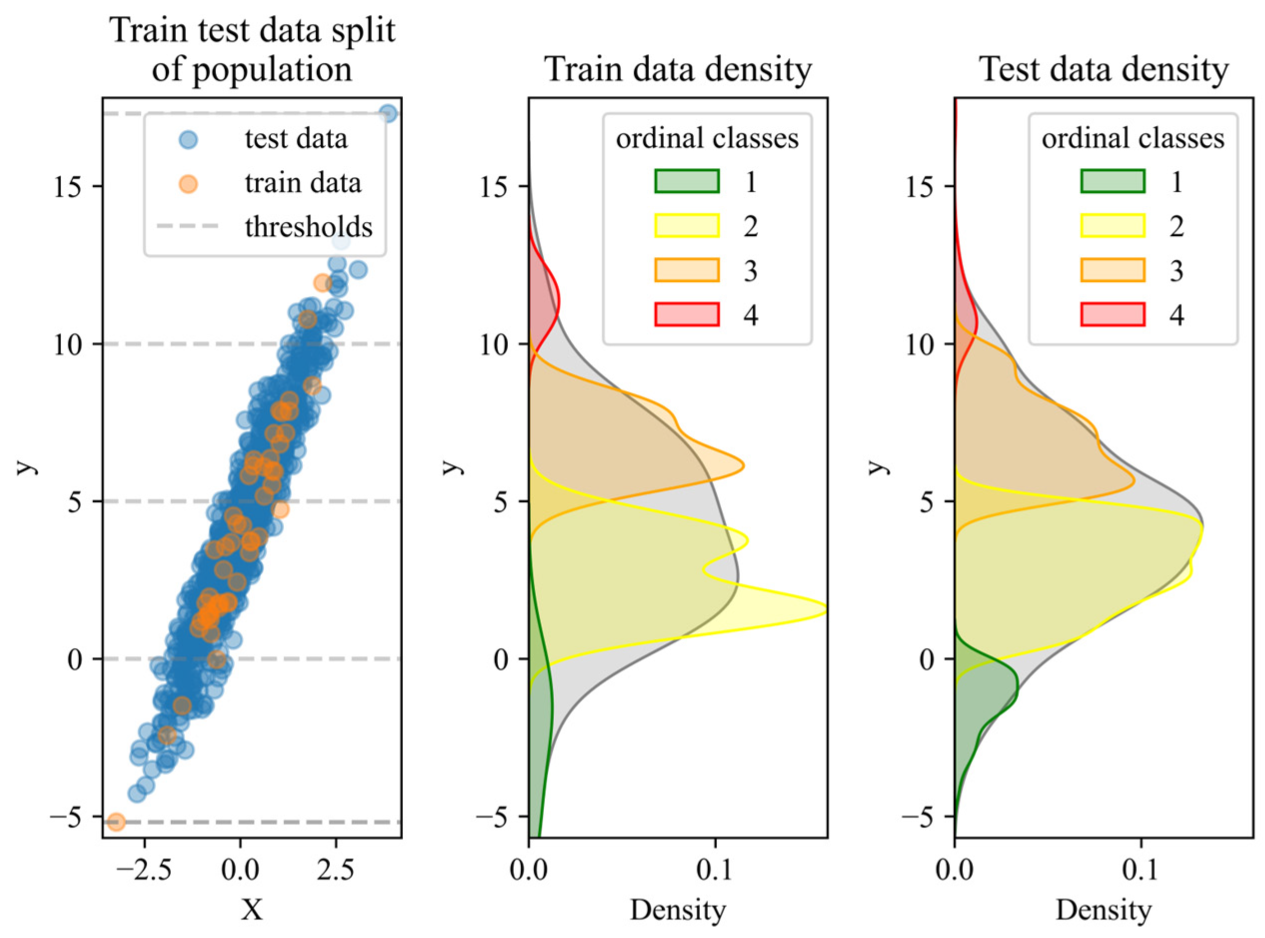
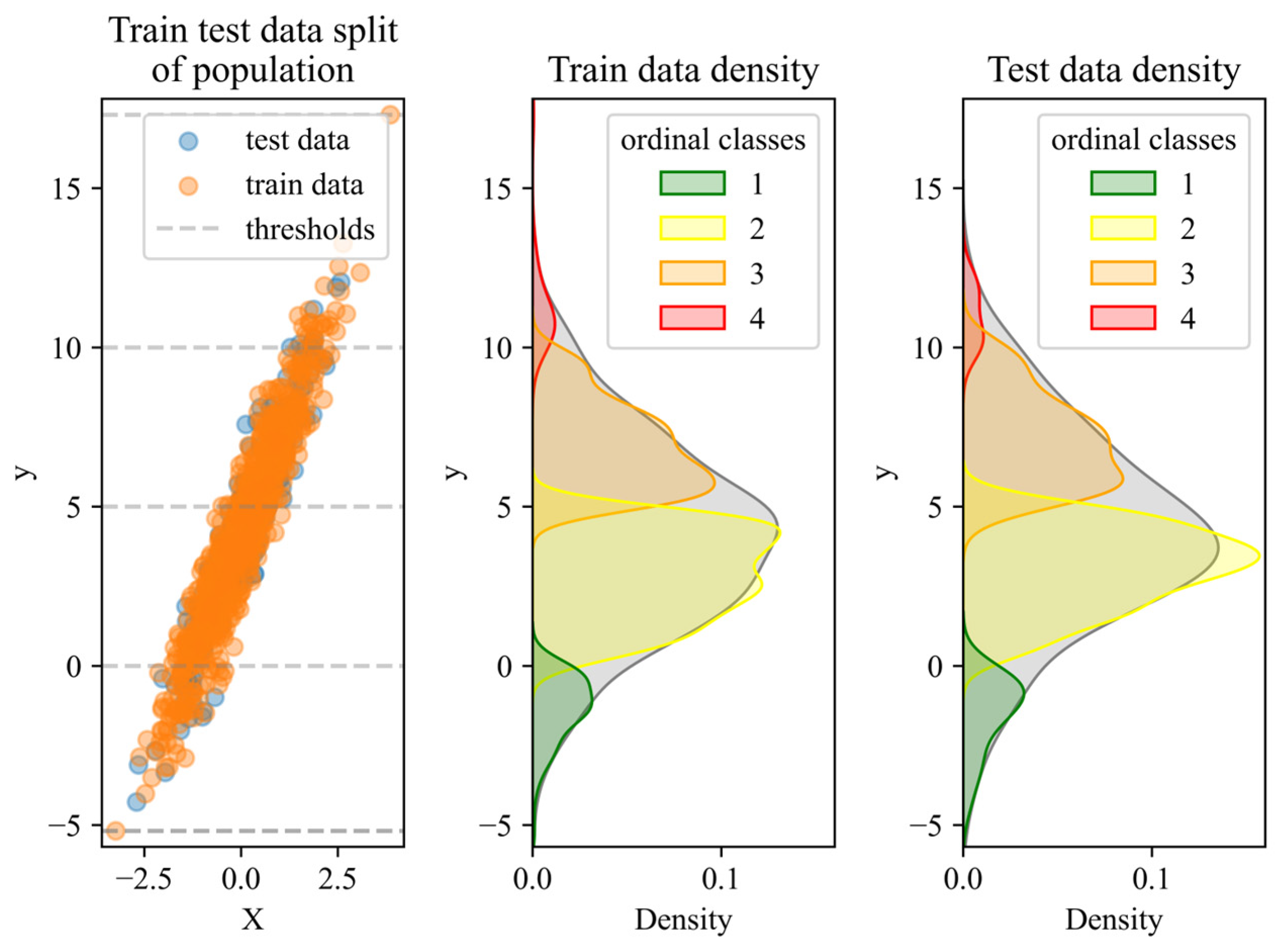
The following figures display the described data in x-y plots, showing the corresponding probability distributions for each class based on the training-test split with 5/95 (Figure 2) and 80/20 ratios (Figure 3).

Figure 2 visually demonstrates that even with just 5% of the training data, the probability distribution is similar to that based on the entire dataset. Increasing the proportion of training data to 80% leads to an even closer approximation of the class distribution from the total data, as shown in Figure 3. However, despite the significantly larger training dataset, there is no exceptionally strong visual improvement in the comparison between Figure 2 and Figure 3. This supports our hypothesis for this application case: with a less complex frequency distribution of $y$, having as little as 5% of the training data can already yield comparably good results for predicting the true value of $y$.

3.5. Analysis and Evaluation

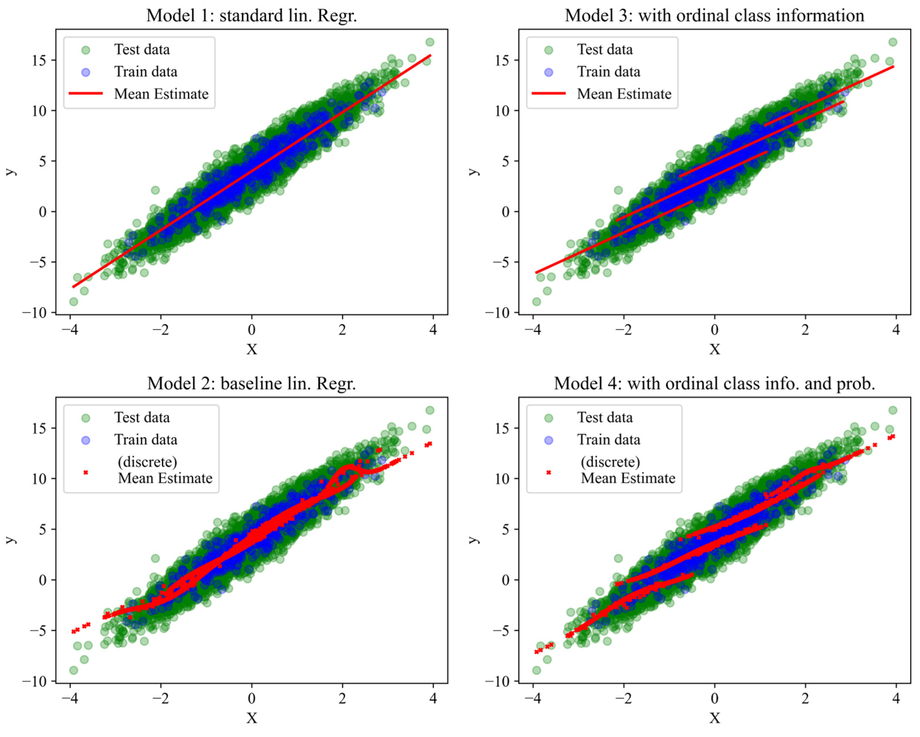
In the detailed analysis, we examine how well the models fit depending on the given features. Figure 4 displays the test and training data along with the linear regression predictions for the out-of-sample forecasts across all feature settings. It is important to note that while linear regression can appear non-linear in the subsequent figures, this is due to the graphical representation being limited to a 2D x-y view. Other influencing factors are still incorporated into the predictions. Therefore, several dimensions (influencing factors) used in the analysis are reduced to two for visual clarity.

Figure 4 illustrates the significant impact of including probability features and, especially, class features on model performance. A visual comparison in 2D between (1) and (4) shows that our method allows for a more flexible (and even seemingly nonlinear) modeling compared to standard linear regression. This is because the hyperplane in multivariate standard linear regression is extended by $2K$ additional planes, where $K$ is the number of classes. In the following

Table 1. Comparison of the different feature input settings (with linear regression) based on the training data proportion for in- and out-of-sample predictions. Evaluation metrics are $MSE$, R², and the computational time (CT). The best results per comparison are highlighted in bold.

Train Data Proportion [in %]	Model	MSE		R2 [%]		CT [s]
		in *	out **	in *	out **
5	1	0.876	1.001	89.47	89.39	1.27
	2	0.646	0.893	92.24	90.53	1.39
	3	0.499	0.594	94.00	93.71	1.90
	4	0.427	0.527	94.86	94.41	1.99
20	1	1.011	0.991	88.41	89.62	1.50
	2	0.724	0.873	91.70	90.85	1.66
	3	0.527	0.544	93.95	94.30	1.45
	4	0.459	0.501	94.73	94.75	1.47
50	1	1.066	0.921	88.19	90.54	1.22
	2	0.739	0.864	91.82	91.11	1.23
	3	0.465	0.594	94.85	93.89	1.25
	4	0.426	0.547	95.28	94.38	1.14
80	1	0.998	0.977	89.09	90.52	1.08
	2	0.730	0.987	92.02	90.42	0.95
	3	0.485	0.691	94.69	93.30	0.87
	4	0.467	0.616	94.89	94.02	0.91

* in-sample. ** out-of-sample.

, we prove this statement with regression evaluation metrics.

The out-of-sample results in Table 1 indicate that expanding the model from input feature setting (1) to (2) leads to a significant reduction in $MSE$ (approximately 5–10%) and an average improvement in $R^2$ of about 1% across all proportions. Notably, as the proportion of training data increases, the benefit from the probability distributions diminishes. This, combined with the in-sample results, suggests that a higher proportion may increase the likelihood of overfitting. However, the new features provide substantial benefits in out-of-sample evaluation, especially when training data are limited (i.e., in small sample size problems). This advantage is also observed in the comparison between settings (3) and (4). The comparison between (1) and (3) is less relevant because the additional categorical variable has a significant impact on the model, making such a comparison less meaningful.

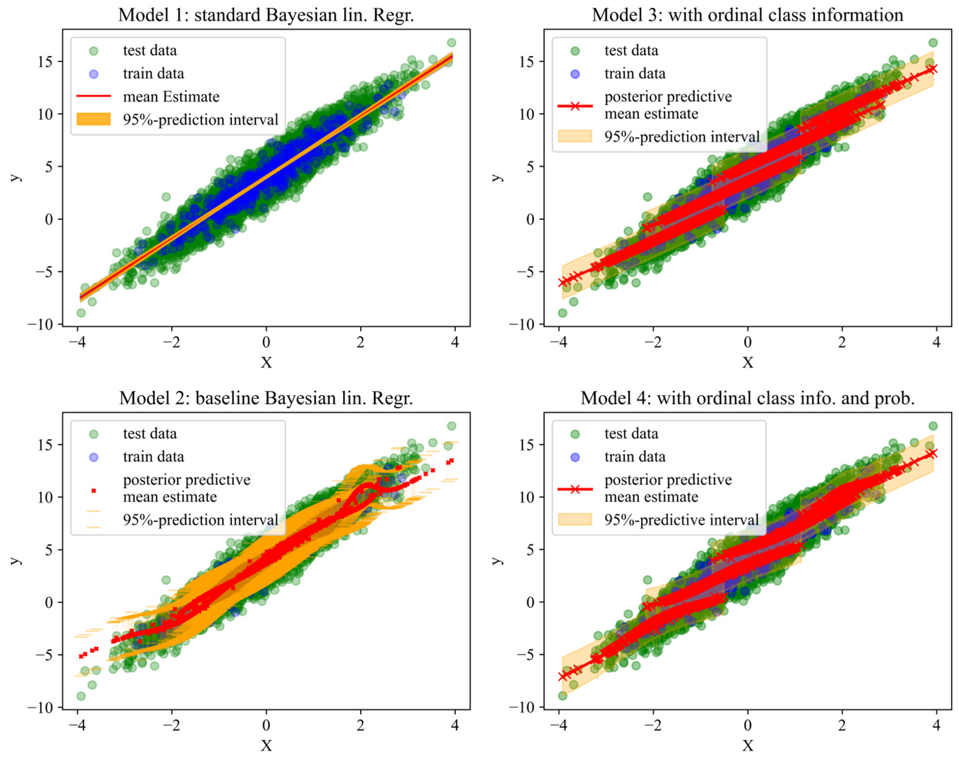
In the next step, we examine the same evaluation considering uncertainties. For Bayesian linear regression, we extend point estimates with a PI. Figure 5 shows, similar to Figure 4, how different feature combinations (1)–(4) affect out-of-sample predictions.

Comparing Figure 5 to Figure 4, the average predictions remain nearly identical. However, when examining the PIs, it becomes apparent that adding probability features increases the uncertainty, as seen in the comparison between models (1) and (2) and between (3) and (4). Nevertheless, the very narrow PI for (1) seems to underestimate the actual uncertainty of the test data.

Regarding Figure 5,

Table 2. Comparison of different feature input settings (using Bayesian linear regression) was conducted by evaluating the coverage of model predictions within the PI (out-of-sample). Evaluation metrics are $coverag{e}_{rate}$, $PI width$, $ratio$, and the computational time $\left(CT\right)$. The best results per comparison are highlighted in bold.

Train Data Proportion [in %]	Input Feature Settings	Pl Metrics			CT [s]
		Cov. Rate [in %]	PI Width	Ratio [in %]
5	1	31.68	1.31	24.25	53.94
	2	53.89	3.75	14.38	56.27
	3	96.21	3.25	29.61	78.09
	4	97.89	3.43	28.55	97.43
20	1	15.13	0.56	27.14	50.89
	2	24.63	1.57	15.66	55.21
	3	96.00	2.96	32.49	96.06
	4	95.63	2.83	33.78	138.68
50	1	9.80	0.40	24.79	50.48
	2	20.80	0.89	23.45	53.81
	3	94.00	2.71	34.66	118.48
	4	93.2	2.62	35.55	191.8
80	1	7.50	0.31	24.34	49.81
	2	15.00	0.62	24.10	54.81
	3	94.00	2.75	34.15	154.44
	4	93.50	2.72	34.37	215.88

confirms that while the absolute coverage rate increases in comparisons between (1) and (2) and between (3) and (4), the coverage relative to the width of the PI (Ratio) generally decreases.

4. Simulation Study

In this section, we examine a more complex simulation study, oriented on a real-world application with respect to variable names and ranges. This approach allows us to gain comprehensive insights into the entire population, unlike using potentially biased or skewed samples. As before, the data are divided into training and test sets.

4.1. Simulation Design

The generated synthetic data include four input features that influence the log-normally distributed target variable. Let $X$ be the feature matrix. This multivariate data problem is designed to simulate a real-world application where, in a street survey, individuals are asked about their age, work experience, education level, weekly hours, and the target variable, salary. A relatively small portion is asked for their exact salary (training data), while the remainder are asked to categorize their salary into ranked (ordinal) classes based on predefined thresholds (test data), such as ‘low income’ or ‘high income’.

For dataset 1, the following equation applies:

$$salary=0.02\ast X_1+0.05\ast X_2+0.1\ast X_3+0.03\ast X_4+{ϵ}_1$$

and for dataset 2:

$$salary=0.03\ast X_1+0.06\ast X_2+0.04\ast X_4+0.1\ast X_5+{ϵ}_2$$

with

$$salary~Log-N(\mu ,{\sigma }^2)$$

and

$$X1: age [in a] ~ U(20,65)$$

$$X2: experience \left[in a\right] ~ U\left(0,40\right)$$

$$X3: educational level ~ U(1,5)$$

$$X4: hours per week \left[in h\right] ~ U(20,60)$$

$$X5: performance rating ~ U(1,6)$$

$${ϵ}_1: noise ~ N\left(0,0.1\right)$$

$${ϵ}_2: noise ~ N(0,0.2).$$

The coefficients are chosen randomly. In the simulation, $n$ samples are drawn such that the input matrix $\dim \left(X\right)=(n\times 4)$. Samples are also randomly drawn and evaluated for $n=3000$ and $n=5000$ for each dataset. For reproducibility, a random seed is used per dataset. Figure 6 shows a simulation example ($n=3000$) with the correlations between the independent and dependent variables on the left and the approximately log-normally distributed target variable (salary) in detail on the right.

The simulation allows us to apply the methodology to a known and thoroughly understandable ground truth. We compare different train-test split ratios of 5/95, 10/90, and 20/80. This simulates the applicability to small sample size problems to re-anonymize ordinal data. Only for the training data, the exact salary values are provided. In the next step, we evaluate the simulated datasets for the application of the methodology.

4.2. Simulation Results

Table 3. Comparison of the different feature input settings (with linear regression) and training data proportion based on the simulation study data for in- and out-of-sample. Evaluation metrics are $MSE$ and $R^2$. The best results per comparison are highlighted in bold.

Dataset	Train Data Proportion	Model	MSE		R2
			in *	out **	in *	out **
1 (# 3000)	5	1	0.00246	0.00358	84.97	80.85
		2	0.00050	0.00118	96.97	93.72
		3	0.00055	0.00113	96.65	93.97
		4	0.00048	0.00130	97.06	93.03
	10	1	0.00366	0.00352	80.16	81.09
		2	0.00111	0.00098	93.98	94.73
		3	0.00104	0.00098	94.39	94.71
		4	0.00092	0.00102	95.00	94.51
	20	1	0.00342	0.00354	80.17	81.30
		2	0.00104	0.00108	93.95	94.30
		3	0.00099	0.00099	94.27	94.75
		4	0.00094	0.00093	94.56	95.07
2 (# 3000)	5	1	0.00488	0.00528	66.18	65.13
		2	0.00054	0.00121	96.25	92.00
		3	0.00059	0.00114	95.92	92.49
		4	0.00053	0.00113	96.32	92.54
	10	1	0.00474	0.00534	66.99	64.89
		2	0.00087	0.00119	93.92	92.20
		3	0.00093	0.00109	93.55	92.84
		4	0.00084	0.00110	94.15	92.80
	20	1	0.00517	0.00523	66.32	65.31
		2	0.00084	0.00138	94.51	90.84
		3	0.00095	0.00109	93.78	92.75
		4	0.00083	0.00130	94.59	91.37
3 (# 5000)	5	1	0.00311	0.00285	80.75	81.05
		2	0.00107	0.00093	93.41	93.86
		3	0.00086	0.00081	94.71	94.59
		4	0.00073	0.00074	95.46	95.10
	10	1	0.00297	0.00287	80.54	81.02
		2	0.00085	0.00082	94.40	94.56
		3	0.00090	0.00080	94.13	94.72
		4	0.00083	0.00075	94.58	95.01
	20	1	0.00316	0.00278	80.19	81.32
		2	0.00124	0.00080	92.20	94.64
		3	0.00104	0.00074	93.50	95.02
		4	0.00098	0.00072	93.88	95.19
4 (# 5000)	5	1	0.00501	0.00497	67.83	66.18
		2	0.00096	0.00107	93.86	92.69
		3	0.00105	0.00103	93.24	92.97
		4	0.00095	0.00107	93.87	92.70
	10	1	0.00403	0.00502	70.46	66.24
		2	0.00052	0.00113	96.17	92.40
		3	0.00062	0.00108	95.46	92.76
		4	0.00051	0.00111	96.28	92.54
	20	1	0.00480	0.00492	66.17	66.91
		2	0.00117	0.00116	91.76	92.24
		3	0.00095	0.00100	93.32	93.30
		4	0.00089	0.00094	93.76	93.69

* in-sample. ** out-of-sample.

shows the evaluation of the six different datasets. Notably, in all cases, using the linear baseline model (2) instead of the standard model (1) provides a significant improvement. This confirms that even without including the ordinal class (3) as a categorical feature, exceptional out-of-sample results can be achieved. In the comparison between models (3) and (4), no substantial improvement was observed. Often, model (4) tends to overfit, indicating that model (3) is sufficiently trained. However, in some cases, such as dataset 3 with 5% training data, an improvement in the out-of-sample R² value by 0.5% was achieved despite the already very good result of ~95%. We conclude that, depending on the data complexity and the SL regression model used, further improvements are possible by incorporating probabilities even when using categories as features. Regarding the MSE, it is also very clear that using probabilities (2) results in a 3–5 times lower MSE compared to standard linear regression (1).

5. Benchmarking

To evaluate real-world applicability, we use multiple datasets from the UCI Database and Kaggle to conduct a benchmark study comparing various feature combinations and models.

5.1. Datasets

For a comprehensive analysis, we select datasets that differ in terms of the ratio between the number of observations and the number of features. We examine two datasets for each category: average, low, and high sample/feature ratio.

Table 4. Descriptive information about class size and thresholds for the multivariate Benchmark datasets.

	Descriptive Analysis of the Target			Class Size	Class Thresholds
	Min	Mean	Max
AutoMPG	9	23.52	46.6	4	[8, 16, 24, 32.5, 48]
Boston Housing	5	22.53	50	4	[4, 15, 25, 35, 51]
Student Performance	0	11.91	19	4	[−1, 9, 12, 15, 20]
Automobile *	-	-	-	2	[−3.5, 1, 3.5]
California Housing	14,999	206,855	500,001	4	[14,998, 136,249, 257,500, 378,751, 500,002]
Bike Sharing	1	189.46	977	4	[0, 150, 350, 500, 1000]

* Automobile has an ordinal-scaled regression target. The target does not have to be metric scaled to further coarsen into classes.

shows the settings for class size and thresholds for each dataset, and

Table 5. Descriptive information for the normalized multivariate Benchmark datasets.

	Samples Size	Features Size	Sample/ Feature- Ratio	Target	Target Unit	Target Mean	Target IQR
AutoMPG	398	8	49.8	MPG	$\left[{\displaystyle \frac{\mathrm{m}\mathrm{i}\mathrm{l}\mathrm{e}\mathrm{s}}{\mathrm{g}\mathrm{a}\mathrm{l}\mathrm{l}\mathrm{o}\mathrm{n}}}\right]$	0.3860	0.3059
Boston Housing	506	14	36.1	MEDV	[1k USD]	0.3896	0.1772
Student Performance	649	57	11.4	G3	Points	0.6266	0.2105
Automobile	205	69	3.0	Risk	Level	0.5668	0.4000
California Housing	20,640	14	1474.3	MHV	[USD]	0.3956	0.2992
Bike Sharing	17,379	14	1241.4	Count	Bikes	0.1931	0.2469

provides additional descriptive information.

5.2. Evaluation

In the evaluation, we use models (1) and (3) as benchmarks for models (2) and (4), respectively, because models (1) and (2) and models (3) and (4) are comparable based on the given input. Looking at

Table 6. Comparison of the different feature input settings (with linear regression) and training data proportion based on the Benchmark datasets for in- and out-of-sample. Evaluation metrics are $MSE$ and $R^2$. The best results per comparison are highlighted in bold.

Dataset	Train Data Proportion	Model	MSE		R2
			in *	out **	in *	out **
AutoMPG	5	1	0.00273	0.01178	92.92	72.77
		2	0.00079	0.00975	97.96	77.47
		3	0.00087	0.00507	97.75	88.28
		4	0.00041	0.03101	98.93	28.36
	10	1	0.00642	0.00938	85.46	78.14
		2	0.00249	0.00398	94.37	90.73
		3	0.00231	0.00362	94.76	91.57
		4	0.00202	0.00528	95.42	87.71
	20	1	0.00625	0.00852	86.02	80.04
		2	0.00155	0.00439	96.52	89.71
		3	0.00167	0.00380	96.27	91.10
		4	0.00130	0.00424	97.10	90.08
Boston Housing	5	1	0.00318	0.01769	92.32	57.55
		2	0.00216	>1	94.79	$<1{ \times 10}^{-5}$
		3	0.00057	0.01033	98.63	75.21
		4	0.00037	0.01878	99.11	54.95
	10	1	0.00349	0.02233	88.87	47.85
		2	0.00147	0.01741	95.32	59.35
		3	0.00122	0.00656	96.11	84.69
		4	0.00093	5.82780	97.03	$<1{ \times 10}^{-5}$
	20	1	0.00653	0.01684	83.81	59.93
		2	0.00258	0.00642	93.59	84.72
		3	0.00185	0.00329	95.40	92.18
		4	0.00165	0.00373	95.91	91.12
Automobile	5	1	$<1{ \times 10}^{-5}$	0.07078	100.00	−12.98
		2	$<1{ \times 10}^{-5}$	0.07211	100.00	−15.10
		3	$<1{ \times 10}^{-5}$	0.06992	100.00	−11.61
		4	$<1{ \times 10}^{-5}$	0.07121	100.00	−13.66
	10	1	$<1{ \times 10}^{-5}$	0.08464	100.00	−36.34
		2	$<1{ \times 10}^{-5}$	0.08549	100.00	−37.70
		3	$<1{ \times 10}^{-5}$	0.05165	100.00	16.80
		4	$<1{ \times 10}^{-5}$	0.05027	100.00	19.04
	20	1	$<1{ \times 10}^{-5}$	0.17308	100.00	−181.87
		2	$<1{ \times 10}^{-5}$	0.14112	100.00	−129.83
		3	$<1{ \times 10}^{-5}$	0.16912	100.00	−175.43
		4	$<1{ \times 10}^{-5}$	0.14078	100.00	−129.27
Student Performance	5	1	$<1{ \times 10}^{-5}$	0.08539	100.00	−197.44
		2	$<1{ \times 10}^{-5}$	0.07496	100.00	−161.09
		3	$<1{ \times 10}^{-5}$	0.02395	100.00	16.56
		4	$<1{ \times 10}^{-5}$	0.02728	100.00	4.99
	10	1	0.00910	0.07507	66.09	−158.08
		2	0.00186	0.03561	93.05	−22.41
		3	0.00151	0.01194	94.37	58.95
		4	0.00100	0.02383	96.27	18.07
	20	1	0.01423	0.03304	47.32	−12.67
		2	0.00403	0.01178	85.06	59.82
		3	0.00312	0.00659	88.43	77.53
		4	0.00305	0.00676	88.70	76.95
California Housing	5	1	0.01949	0.02040	65.61	63.96
		2	0.00497	0.00532	91.23	90.60
		3	0.00382	0.00389	93.27	93.12
		4	0.00381	0.00389	93.28	93.13
	10	1	0.01783	0.02049	68.19	63.84
		2	0.00455	0.00518	91.87	90.87
		3	0.00366	0.00384	93.48	93.22
		4	0.00363	0.00386	93.52	93.19
	20	1	0.01969	0.02027	64.68	64.32
		2	0.00521	0.00523	90.65	90.80
		3	0.00371	0.00381	93.35	93.29
		4	0.00369	0.00380	93.37	93.31
Bike Sharing	5	1	0.02051	0.02143	40.93	37.93
		2	0.00343	0.00339	90.13	90.17
		3	0.00255	0.00297	92.65	91.41
		4	0.00249	0.00296	92.84	91.43
	10	1	0.02122	0.02117	39.20	38.63
		2	0.00333	0.00347	90.47	89.94
		3	0.00282	0.00294	91.93	91.48
		4	0.00280	0.00292	91.98	91.53
	20	1	0.02141	0.02111	39.42	38.52
		2	0.00411	0.00371	88.36	89.19
		3	0.00295	0.00291	91.65	91.54
		4	0.00291	0.00289	91.78	91.60

* in-sample. ** out-of-sample.

, it is evident that the use of probability distributions as additional input in model (2) often provides a significant improvement compared to standard models (1). This also holds true in comparisons between (1) and (3). However, when comparing models (2) and (3), their performance is often comparable. Specific exceptions include the Boston Housing dataset for 5% and 10% training data, where the use of probability distributions with models (2) and (4) confuses the model, which results in worse results. Comparing models (3) and (4) confirms that overfitting is a concern, particularly with model (4). The datasets for Automobile and Student Performance highlight a key limitation of both linear regression and our new approach: models with a low sample-to-feature ratio struggle to produce reliable results, even when probabilistic features are incorporated. In these cases, our method combined with linear regression reaches its limits. This limitation is particularly evident in the Student Performance dataset, where increasing the proportion of training data leads to improved model results. This suggests that a low sample-to-feature ratio significantly restricts performance. A similar trend is observed in the AutoMPG and Boston Housing datasets, which have a moderately higher sample-to-feature ratio. While we observe improvements from model (1) to (2) and even (3), model (4) appears to overfit, occasionally yielding exceptionally poor results. In contrast, model (4) achieved the best results across all evaluations for the California Housing and Bike Sharing datasets. This demonstrates that, when well calibrated, the use of probabilistic features can marginally improve performance compared to the categorical variable model (3).

6. Conclusions and Discussion

This paper aimed to explore the feasibility of tracing anonymized data from very small sample sizes. We developed a methodology that combines latent probabilistic distributions over ordinal classes—i.e., anonymized data—with a small sample approach. This combination enables significantly improved predictions of actual values using linear regression, applicable to both simple and complex data structures. In the context of increasing data protection concerns, our new method demonstrates how standard anonymization techniques, such as discretizing metric data in street surveys or similar contexts, can be accurately reversed. While it might seem counterintuitive to infer exact values from discrete classes using latent distributions, this approach aligns with existing methodologies. The use of distributions to describe latent relationships within a class provides notable advantages.

Our application results show that even a small training dataset can outperform standard linear regression when using latent probabilistic distributions. However, when comparing models that include ordinal class variables, probabilistic distributions often do not provide substantial additional benefits and may even lead to overfitting. This methodology is particularly versatile for any supervised learning regression task. While data quantity and quality can be limited, the approach remains effective. One limitation is that latent probabilistic distributions require a minimum amount of data, which, in our cases, did not need to be excessively large.

Future research should focus on a more detailed examination of the distribution of latent influencing factors, while considering the potential for optimizing class boundaries. Considering the significant impact of class boundaries, combining the optimal clustering solution and given class boundaries could further improve the methodology.

This paper used normally distributed modeling of ordinal classes and considered these as influencing features. Future work could explore more detailed modeling with Gaussian mixture models or other distributions.

Overall, beyond data protection and anonymization, our approach offers universal applicability and could improve various supervised learning regression problems, particularly when latent probabilistic distributions are not independently or sufficiently recognized by the model.

References

1. Lubarsky, B. Re-Identification of “Anonymized Data”. Georg. Law Technol. Rev. 2010. Available online: https://www.georgetownlawtechreview.org/re-identification-of-anonymized-data/GLTR-04-2017 (accessed on 10 September 2021).
2. Porter, C.C. De-Identified Data and Third Party Data Mining: The Risk of Re-Identification of Personal Information. Shidler JL Com. Tech. 2008, 5, 1. [Google Scholar]
3. Senavirathne, N.; Torra, V. On the Role of Data Anonymization in Machine Learning Privacy. In Proceedings of the 2020 IEEE 19th International Conference on Trust, Security and Privacy in Computing and Communications (TrustCom), Guangzhou, China, 29 December 2020–1 January 2021; pp. 664–675. [Google Scholar]
4. Ercikan, K. Limitations in Sample-to-Population Generalizing. In Generalizing from Educational Research; Routledge: Abingdon, UK, 2008; ISBN 978-0-203-88537-6. [Google Scholar]
5. Hertzog, M.A. Considerations in Determining Sample Size for Pilot Studies. Res. Nurs. Health 2008, 31, 180–191. [Google Scholar] [CrossRef]
6. Li, T.; Li, N.; Zhang, J. Modeling and Integrating Background Knowledge in Data Anonymization. In Proceedings of the 2009 IEEE 25th International Conference on Data Engineering, Shanghai, China, 29 March–2 April 2009; pp. 6–17. [Google Scholar]
7. Stickland, M.; Li, J.D.-Y.; Tarman, T.D.; Swiler, L.P. Uncertainty Quantification in Cyber Experimentation; Sandia National Lab. (SNL-NM): Albuquerque, NM, USA, 2021. [Google Scholar]
8. Oertel, H.; Laurien, E. Diskretisierung. In Numerische Strömungsmechanik; Vieweg+Teubner Verlag: Wiesbaden, Germany, 2003; pp. 126–214. ISBN 978-3-528-03936-3. [Google Scholar]
9. Senavirathne, N.; Torra, V. Rounding Based Continuous Data Discretization for Statistical Disclosure Control. J. Ambient Intell. Humaniz. Comput. 2023, 14, 15139–15157. [Google Scholar] [CrossRef]
10. Inan, A.; Kantarcioglu, M.; Bertino, E. Using Anonymized Data for Classification. In Proceedings of the 2009 IEEE 25th International Conference on Data Engineering, Shanghai, China, 29 March–2 April 2009; pp. 429–440. [Google Scholar]
11. Pors, S.J. Using Discretization and Resampling for Privacy Preserving Data Analysis: An Experimental Evaluation. Master’s Thesis, Utrecht University, Utrecht, The Netherlands, 2018. [Google Scholar]
12. Milani, M.; Huang, Y.; Chiang, F. Data Anonymization with Diversity Constraints. IEEE Trans. Knowl. Data Eng. 2021, 35, 3603–3618. [Google Scholar] [CrossRef]
13. Bayardo, R.J.; Agrawal, R. Data Privacy through Optimal K-Anonymization. In Proceedings of the 21st International Conference on Data Engineering (ICDE’05), Tokyo, Japan, 5–8 April 2005; pp. 217–228. [Google Scholar]
14. Robitzsch, A. Why Ordinal Variables Can (Almost) Always Be Treated as Continuous Variables: Clarifying Assumptions of Robust Continuous and Ordinal Factor Analysis Estimation Methods. Front. Educ. 2020, 5, 589965. [Google Scholar] [CrossRef]
15. Zouinina, S.; Bennani, Y.; Rogovschi, N.; Lyhyaoui, A. A Two-Levels Data Anonymization Approach. In Artificial Intelligence Applications and Innovations; Maglogiannis, I., Iliadis, L., Pimenidis, E., Eds.; IFIP Advances in Information and Communication Technology; Springer International Publishing: Cham, Switzerland, 2020; Volume 583, pp. 85–95. ISBN 978-3-030-49160-4. [Google Scholar]
16. Xin, G.; Xiao, Y.; You, H. Discretization of Continuous Interval-Valued Attributes in Rough Set Theory and Its Application. In Proceedings of the 2007 International Conference on Machine Learning and Cybernetics, Hong Kong, China, 19–22 August 2007; Volume 7, pp. 3682–3686. [Google Scholar]
17. Rhemtulla, M.; Brosseau-Liard, P.É.; Savalei, V. When Can Categorical Variables Be Treated as Continuous? A Comparison of Robust Continuous and Categorical SEM Estimation Methods under Suboptimal Conditions. Psychol. Methods 2012, 17, 354. [Google Scholar] [CrossRef]
18. Jorgensen, T.D.; Johnson, A.R. How to derive expected values of structural equation model parameters when treating discrete data as continuous. Struct. Equ. Model. A Multidiscip. J. 2022, 29, 639–650. Available online: https://scholar.google.de/scholar?hl=de&as_sdt=0%2C5&q=Jorgensen%2C+T.D.%3B+Johnson%2C+A.R.+How+to+Derive+Expected+Values+of+Structural+Equation+Model+Parameters+When+Treating+Discrete+Data+as+Continuous.&btnG= (accessed on 10 October 2024). [CrossRef]
19. Zhou, B.; Pei, J.; Luk, W. A Brief Survey on Anonymization Techniques for Privacy Preserving Publishing of Social Network Data. ACM Sigkdd Explor. Newsl. 2008, 10, 12–22. [Google Scholar] [CrossRef]
20. Murthy, S.; Bakar, A.A.; Rahim, F.A.; Ramli, R. A Comparative Study of Data Anonymization Techniques. In Proceedings of the 2019 IEEE 5th Intl Conference on Big Data Security on Cloud (BigDataSecurity), IEEE Intl Conference on High Performance and Smart Computing,(HPSC) and IEEE Intl Conference on Intelligent Data and Security (IDS), Washington, DC, USA, 27–29 May 2019; pp. 306–309. [Google Scholar]
21. Mogre, N.V.; Agarwal, G.; Patil, P. A Review on Data Anonymization Technique for Data Publishing. Int. J. Eng. Res. Technol. IJERT 2012, 1, 1–5. [Google Scholar]
22. Kaur, P.C.; Ghorpade, T.; Mane, V. Analysis of Data Security by Using Anonymization Techniques. In Proceedings of the 2016 6th International Conference-Cloud System and Big Data Engineering (Confluence), Noida, India, 14–15 January 2016; pp. 287–293. [Google Scholar]
23. Martinelli, F.; SheikhAlishahi, M. Distributed Data Anonymization. In Proceedings of the 2019 IEEE Intl Conf on Dependable, Autonomic and Secure Computing, Intl Conf on Pervasive Intelligence and Computing, Intl Conf on Cloud and Big Data Computing, Intl Conf on Cyber Science and Technology Congress (DASC/PiCom/CBDCom/CyberSciTech), Fukuoka, Japan, 5–8 August 2019; pp. 580–586. [Google Scholar]
24. Marques, J.F.; Bernardino, J. Analysis of Data Anonymization Techniques. In Proceedings of the KEOD 2020—12th International Conference on Knowledge Engineering and Ontology Development, Online Streaming, 2–4 November 2020; pp. 235–241. [Google Scholar]
25. Abd Razak, S.; Nazari, N.H.M.; Al-Dhaqm, A. Data Anonymization Using Pseudonym System to Preserve Data Privacy. IEEE Access 2020, 8, 43256–43264. [Google Scholar] [CrossRef]
26. Muthukumarana, S.; Swartz, T.B. Bayesian Analysis of Ordinal Survey Data Using the Dirichlet Process to Account for Respondent Personality Traits. Commun. Stat.-Simul. Comput. 2014, 43, 82–98. [Google Scholar] [CrossRef]
27. Sha, N.; Dechi, B.O. A Bayes Inference for Ordinal Response with Latent Variable Approach. Stats 2019, 2, 321–331. [Google Scholar] [CrossRef]
28. Cox, D.R. Note on Grouping. J. Am. Stat. Assoc. 1957, 52, 543–547. [Google Scholar] [CrossRef]
29. Fang, K.-T.; Pan, J. A Review of Representative Points of Statistical Distributions and Their Applications. Mathematics 2023, 11, 2930. [Google Scholar] [CrossRef]
Figure 1. Mean squared error (MSE) and Jensen-Shannon divergence (J-S divergence) as evaluation metrics for comparing KDE-modeled distributions between test data proportions and the population. The train-test split is performed based on the x-range values. The blue line represents the mean result of the evaluation based on repeated train-test splits, while the orange line indicates the corresponding standard deviation.
Stats 07 00070 g001
Figure 2. Comparison of KDE-modeled distributions for a 5/95 train-test split of the population (depicted by the gray distribution). The distributions are modeled based on values within the respective thresholds for each ordinal class using training data (middle inset) and test data (right inset). The test and training datasets are split randomly but with class stratification. Despite the visually apparent lower dispersion in the training data, the variability of both datasets is similar.
Stats 07 00070 g002
Figure 3. Comparison of KDE-modeled distributions for an 80/20 train-test split (i.e., standard cross validation ratio) of the population (gray distribution). The distributions are modeled based on values within the respective thresholds for each ordinal class, using train data (middle inset) and test data (right inset). The test and training datasets are split randomly but with class stratification.
Stats 07 00070 g003
Figure 4. Comparison of four linear regression models based on different input features for a 5/95 train-test split. The insets show a 2D cross-section of the multivariate models, where all features are used. The test and training datasets are split randomly but with class stratification. Despite the visually apparent lower dispersion in the training data, the variability of both datasets is similar.
Stats 07 00070 g004
Figure 5. Comparison of four Bayesian linear regression models based on different input features for a 5/95 train-test split. The insets show a 2D cross-section of the multivariate models, where all features are used. The test and training datasets are split randomly but with class stratification. Despite the visually apparent lower dispersion in the training data, the variability of both datasets is similar.
Stats 07 00070 g005
Figure 6. Heatmap and histogram with an approximated log-normal distribution for a simulated example with n = 3000 .
Stats 07 00070 g006