Article

Hierarchical Time Series Forecasting of Fire Spots in Brazil: A Comprehensive Approach

by
Ana Caroline Pinheiro
1,2 and
Paulo Canas Rodrigues
1,2,*
1
Department of Statistics, Federal University of Bahia, Salvador 40170-115, BA, Brazil
2
Statistical Learning Laboratory (SaLLy), Federal University of Bahia, Salvador 40170-115, BA, Brazil
*
Author to whom correspondence should be addressed.
Stats 2024, 7(3), 647-670; https://doi.org/10.3390/stats7030039
Submission received: 9 May 2024 / Revised: 24 June 2024 / Accepted: 24 June 2024 / Published: 27 June 2024
(This article belongs to the Special Issue Modern Time Series Analysis II)

Abstract

:
This study compares reconciliation techniques and base forecast methods to forecast a hierarchical time series of the number of fire spots in Brazil between 2011 and 2022. A three-level hierarchical time series was considered, comprising fire spots in Brazil, disaggregated by biome, and further disaggregated by the municipality. The autoregressive integrated moving average (ARIMA), the exponential smoothing (ETS), and the Prophet models were tested for baseline forecasts, and nine reconciliation approaches, including top-down, bottom-up, middle-out, and optimal combination methods, were considered to ensure coherence in the forecasts. Due to the need for transformation to ensure positive forecasts, two data transformations were considered: the logarithm of the number of fire spots plus one and the square root of the number of fire spots plus 0.5. To assess forecast accuracy, the data were split into training data for estimating model parameters and test data for evaluating forecast accuracy. The results show that the ARIMA model with the logarithmic transformation provides overall better forecast accuracy. The BU, MinT(s), and WLS(v) yielded the best results among the reconciliation techniques.

1. Introduction

Forest fires are a recurring problem in Brazil, with 222,798 fire spots recorded nationwide in 2020 [1]. These wildfires significantly impact the ecosystem, infrastructure, and population. The Brazilian biomes host a rich biodiversity that can be partially lost due to these fires. Amazon forest fires substantially affect air quality and public health [2]. The quality and quantity of water can also be affected if the fires reach the vegetation around watersheds. Fires can impact crops and, in the long term, compromise food production if soil fertility is affected by the flames [1]. Producing statistics regarding fire spots is crucial for implementing more efficient control measures. Forecasting forest fires is pivotal in designing effective policies for preventing and controlling these phenomena [3].
The number of fire spots can be expressed as a time series, whether at the municipal, biome, state, or national level. Several studies have analyzed and forecast time series related to the number of fire spots in Brazil. For example, ref. [4] used multiple linear regression and non-seasonal ARIMA techniques associated with meteorological variables to model and forecast forest fires in the Pantanal of Mato Grosso do Sul in Corumbá. The logarithm of the number of fire spots was introduced as the dependent variable, and maximum temperature, relative humidity, and solar radiation were introduced as independent variables. The results showed that the ARIMA model was more suitable for modeling and predicting forest fires [4]. Another study, conducted in the same location, used artificial neural networks (ANNs) to forecast the number of fire spots and showed that it was possible to predict the number of fire spots with a predictive power of 84.8% using a set of meteorological variables as predictors, and 99.4% using only the time series of the number of fire spots as a predictor [5]. However, existing studies on fire spot forecasting have been conducted for specific biomes and/or regions, with no study considering making forecasts for all municipalities and biomes in Brazil.
Moreover, the number of fire spots per municipality, biome, and Brazilian territory can be organized hierarchically to form a hierarchical time series (HTS), which refers to a time series that can be aggregated at different levels based on products, geography, or other characteristics [6,7,8]. An example of a hierarchical time series is the sales of a particular item in a country, where total sales can be disaggregated by state, and each state’s sales can further be disaggregated by municipality. Forecasting hierarchical time series is typically done for all levels, and they should be “coherent”, meaning that aggregate forecasts should be equal to the sum of the corresponding disaggregated forecasts [9]. For instance, the sales forecast for a product in municipalities should result in state-level sales, and the sum of state-level forecasts should equal the total sales forecast for the country.
The first methods for forecasting reconciliation in hierarchical time series (HTS) were the top-down, the bottom-up, and the middle-out. These involve generating forecasts for one aggregation level and then using them to create coherent forecasts for the other levels. The bottom-up approach requires forecasts for all series at the lowest level, which are then aggregated to obtain higher-level forecasts. The top-down method requires a forecast only for the total series, which will be disaggregated to obtain forecasts for the other series at lower levels. The middle-out approach combines the bottom-up and top-down approaches to make forecasts. There is no consensus in the literature on which method is more efficient, as it may depend on the number of series in the hierarchy and the data quality [10].
More recently, methods have emerged that use all aggregation levels to generate coherent forecasts. These methods combine forecasts for all levels to provide the best aggregate forecasts [6] and are known as optimal combination or optimal reconciliation [10,11]. This approach requires estimating the variance and covariance matrix of forecast errors, leading to five variations of this method [9].
To generate coherent forecasts, individual forecasts of the series in the hierarchy are needed without considering any constraints; these are called incoherent forecasts or base forecasts. This paper considers three widely used methods for generating the base forecasts. Exponential smoothing, known as ETS [12,13,14], forecasts the time series as a weighted average of past observations, with weights exponentially decreasing as observations move away from the end of the series. The autoregressive integrated moving average (ARIMA) model generates forecasts based on the autocorrelation of the data. The Prophet, created by Facebook, generates forecasts considering a trend component, seasonality, a component capturing holiday effects, and an error term [15].
Therefore, this study aims to forecast the number of fire spots for each Brazilian municipality, biome, and whole territory by considering different reconciliation techniques and base forecast methods in a three-level hierarchical time series structure. The number of fire spots between January 2011 and December 2022 was obtained from the Brazilian National Institute for Space Research (INPE) and organized by [16]. The autoregressive integrated moving average (ARIMA), the exponential smoothing (ETS), and the Prophet models were tested for baseline forecasts, and nine reconciliation approaches, including top-down, bottom-up, middle-out, and optimal combination methods, were considered to ensure coherence in the forecasts.
The rest of this paper is organized as follows. Section 2 describes the data, the methodology behind hierarchical time series and reconciliation techniques, the models used to obtain the base forecasts, and the accuracy measures used to compare the competing models. Section 3 presents a descriptive and exploratory analysis of the data, followed by the results of the accuracy measures for each model. Finally, Section 4 presents the concluding remarks of the study.

2. Materials and Methods

2.1. The Data

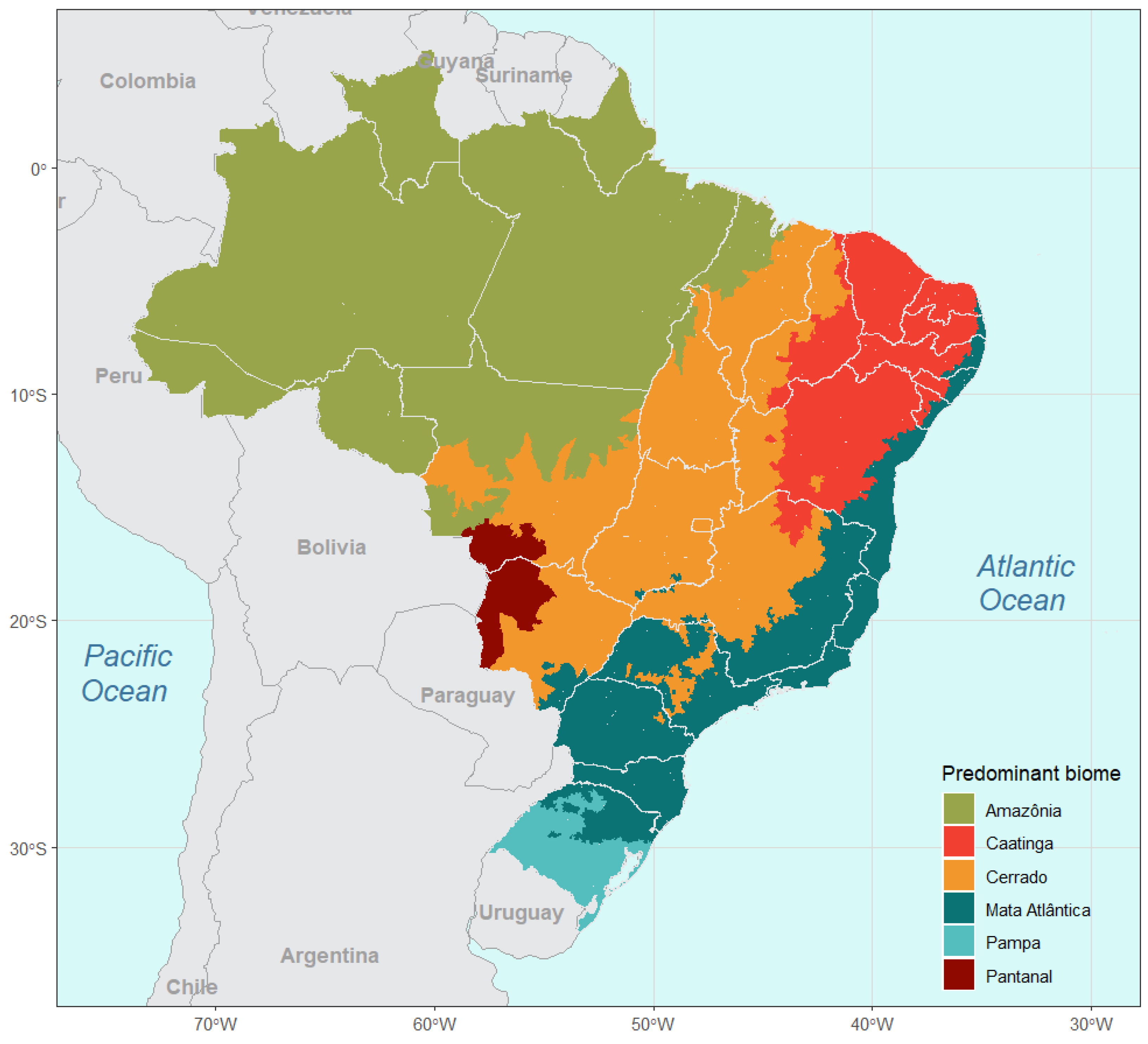
The data used in this study were provided by the QUEIMADAS program of the Brazilian National Institute for Space Research (INPE). The dataset contains the number of fire spots per month in each municipality in Brazil from January 2011 to December 2022 and was organized and made available by [16]. The Brazilian territory is divided into six biomes: (i) Amazônia, encompassing approximately 60% of the world’s largest rainforest, rich in mineral reserves, and providing 20% of the world’s water supply; (ii) Caatinga, featuring a semi-arid climate with remarkable biological diversity and unique species; (iii) Cerrado, acknowledged as the world’s richest savanna in terms of biodiversity, which remained largely unchanged until the 1950s when the federal capital was moved to Brasília; (iv) Mata Atlântica, situated along the Brazilian coast and considered the most endangered biome in the country, with only 27% of the original forest cover still preserved; (v) Pampas, characterized by a rainy climate without a dry period and negative temperatures during winter; and (vi) Pantanal, recognized as the planet’s most extensive continuous floodplain.
The Brazilian municipalities composed of more than one biome were associated with the predominant biome based on the results of a Brazilian Agricultural Research Corporation (Embrapa) project [17]. Figure 1 shows the locations of each of the six biomes in the Brazilian territory.

2.2. Hierarchical Time Series

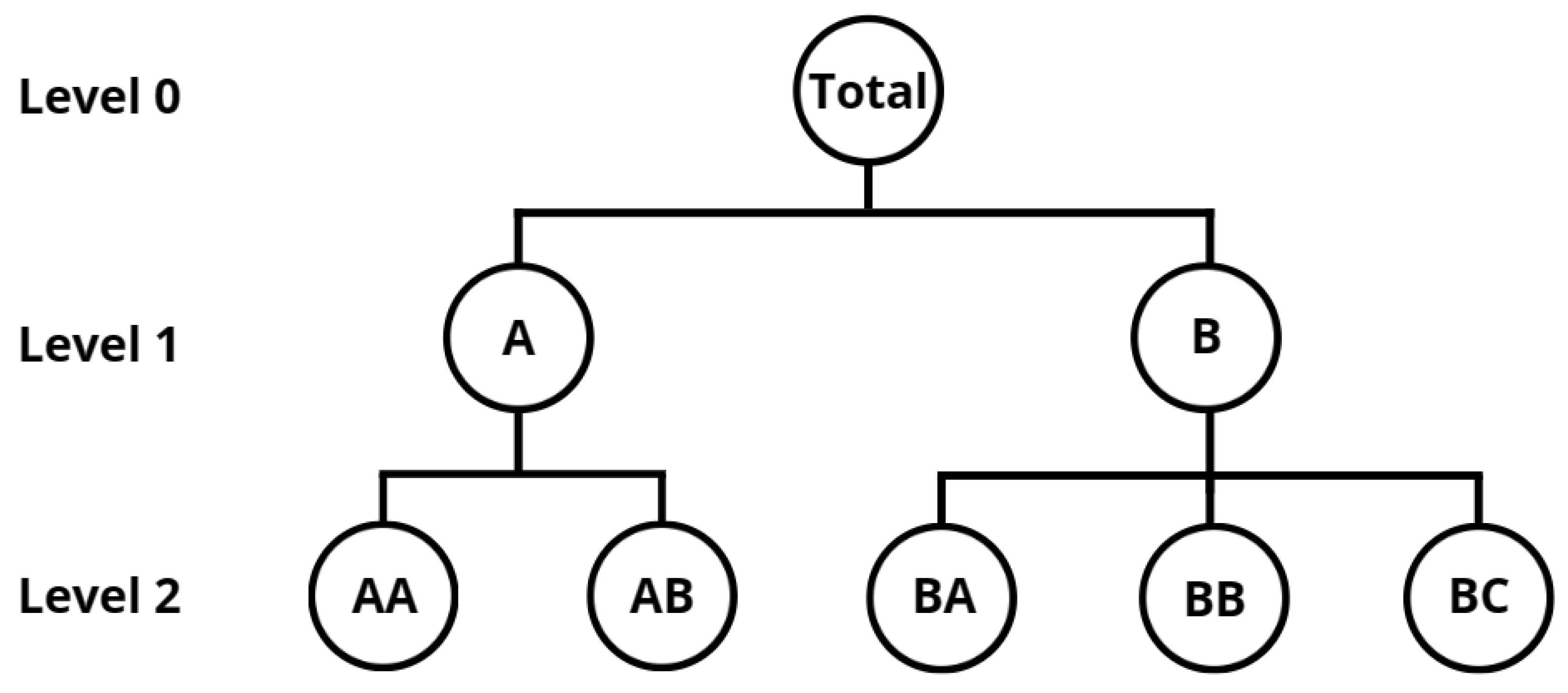
A hierarchical time series is a time series that can be disaggregated into various attributes and different levels. An example of a hierarchical time series is the sales of a specific item in a country, where total sales can be disaggregated by state, and municipalities can further disaggregate each state’s sales. Figure 2 illustrates a hierarchical time series with three levels: Total, which is disaggregated into two time series, A and B, and these are further disaggregated into two (AA and AB) and three (BA, BB, and BC) time series, respectively.
In a hierarchical time series, obtaining observations at time t is possible by summing the observations from the level below. Considering the series in Figure 2, we have the following equations,
y t = y A , t + y B , t ,
y A , t = y A A , t + y A B , t and y B , t = y B A , t + y B B , t + y B C , t ,
Substituting (2) into (1) we get
y t = y A A , t + y A B , t + y B A , t + y B B , t + y B C , t ,
where y t is the total of the time series in the time point t, t = 1 , 2 , T .
The equations above can be written in matrix form as follows:
y t y A , t y B , t y A A , t y A B , t y B A , t y B B , t y B C , t = 1 1 1 1 1 1 1 0 0 0 0 0 1 1 1 1 0 0 0 0 0 1 0 0 0 0 0 1 0 0 0 0 0 1 0 0 0 0 0 1 y A A , t y A B , t y B A , t y B B , t y B C , t ,
that simplifies as:
y t = Sb t ,
where y is an n-dimensional vector of all observations at time t, S is the n × m sum matrix, and b t is an m-dimensional vector of all observations at the lower level of the series at time t.

2.3. Forecasting Approaches for Hierarchical Time Series

It is possible to represent all forecasting methods using a single matrix notation:
y ˜ h = SG y ^ h ,
where y ˜ h represents the coherent forecasts, S is the sum matrix, y ^ h is the base forecasts for all time series in the hierarchy, and G is the matrix mapping the base forecasts, varying in each approach. The following sections briefly describe the different approaches to obtaining coherent forecasts for a hierarchical time series that will be considered in this paper.

2.3.1. Bottom-Up (BU) Approach

The bottom-up (BU) approach involves making forecasts for each time series at the lowest level and then aggregating/summing them to obtain forecasts for the higher levels. The advantage of this method lies in utilizing all available information because the forecasts are made at the lowest level. However, data at the lowest level can be quite noisy, leading to inaccurate forecasts. We can represent this approach using the general form of Equation (4), as follows:
G = [ 0 m × ( n m ) | I m ] ,
where 0 m × ( n m ) is a null matrix and I m is the identity matrix. The matrix G , mapping the base forecasts, is an identity matrix, as the individual forecasts are directly used as coherent forecasts for the higher levels. The bottom-up approach is useful when the lower levels of the hierarchy significantly contribute to the higher levels or when the data quality at the lower levels is more reliable.

2.3.2. Top-Down (TD) Approach

The top-down (TD) method, or top-down forecasting, involves forecasting the total series and then disaggregating it to the lower levels. For this purpose, proportions p 1 , p 2 , , p m are used to determine how these forecasts will be distributed to obtain the forecast for the lower series. This approach has the advantage of simplicity, as it uses only one series to generate forecasts, which also results in significant information loss [10]. In this approach, the matrix G in Equation (3) takes the following form:
G = [ p | 0 m × ( n 1 ) ] ,
where p = [ p 1 , p 2 , , p m ] is a set of proportions. There are different approaches to obtaining these proportions; ref. [18] propose two: average historical proportions and proportions of the historical averages. The top-down (TD) approach in forecasting hierarchical time series is useful when there is insufficient or unreliable data at the lower levels of the hierarchy, making it challenging to model individual series accurately or when straightforward and computationally efficient forecasting methods are preferred.
The average historical proportions are computed as follows.
p j = 1 T t = 1 T y j , t y t j = 1 , , m ,
where p j represents the historical average proportions of the lower series y j , t in relation to y t . In the results of this paper, this approach is denoted as TDAP.
The proportions of the historical averages are obtained as follows.
p j = t = 1 T y j , t T / t = 1 T y t T j = 1 , , m ,
where p j represents the historical average value of the lower-level series y j , t in relation to the mean of y t . In the results of this paper, this approach is denoted as TDPA.
The methods described by Gross and Sohl take into account historical proportions but do not consider how these proportions may change over time, which can impact the accuracy of forecasts for lower levels. To address this, ref. [19] proposed the “Forecast Proportions”, where forecasts for the lower levels are used to calculate the proportions to be applied. The proportions are calculated as follows:
p j = 𝓁 = 0 K 1 y ^ j , h ( 𝓁 ) S ^ j , h ( 𝓁 + 1 )
where y ^ j , h ( 𝓁 ) is the h-step ahead forecast of the series corresponding to the node that is levels above j, and S ^ j , h ( 𝓁 + 1 ) is the sum of the base forecast h steps ahead below the node that is levels above j, which is directly connected to that node. This approach was denoted as TDFP.

2.3.3. Middle-Out (MO) Approach

In the middle-out approach, or intermediate approach, an intermediate level is chosen, and forecasts are generated for all series at that level. Using these forecasts, the bottom-up approach is applied to the levels above the intermediate level, and the top-down approach is applied to the levels below the intermediate level. This strategy aims to strike a balance between the detailed insights provided by the bottom-up method and the high-level overview offered by the top-down method. The choice of the intermediate level is crucial and may vary depending on the specific characteristics of the time series data and the hierarchy structure.

2.3.4. Minimum Trace (MinT) Optimal Reconciliation Approach

The minimum trace (MinT) optimal reconciliation approach optimally combines base forecasts to produce coherent forecasts. Unlike other approaches, it utilizes all information in the hierarchy to generate unbiased forecasts at all levels of the hierarchy [19]. It involves finding the matrix G that minimizes the variances of errors in coherent forecasts y ˜ h , as demonstrated by [9]. The matrix of variance and covariance of errors in coherent forecasts h steps ahead is given by:
V h = V a r [ y T + h y ˜ h ] = SGW h G S ,
where W h = V a r [ y T + h y ^ h ] is the variance–covariance matrix of base forecast errors. Minimizing the variances of errors in coherent forecasts is equivalent to minimizing the trace of the matrix V h , hence the name minimum trace. The matrix G that minimizes the trace of the matrix V h is
G = ( S W h 1 S ) 1 S W h 1 ,
provided that SGS = S is satisfied. Therefore,
y ˜ h = S ( S W h 1 S ) 1 S W h 1 y ^ h .
To obtain y ˜ h , it is necessary to estimate the matrix W h . Several approximations have been proposed, giving rise to various approaches. The five main ones are listed below:
1.
W h = k h I for k h > 0 , transforms MinT into an ordinary least squares (OLS) estimator and assumes that the matrix G is independent of the data, facilitating calculations [6]. However, it assumes independence, leading to information loss.
2.
W h = k h diag ( W ^ 1 ) for all h, where k h > 0 and
W ^ 1 = 1 T t = 1 T e t e t ,
where e t is an n-dimensional vector of residuals from the model generating base forecasts. This approach scales base forecasts using the variance of residuals. In this case, W h can be described as the weighted least squares (WLS) estimator [20]. In the results, this approach is denoted as WLS(v).
3.
W h = k h Λ for all h, where k h > 0 , Λ = diag ( S 1 ) , and 1 is a unit vector of dimension m. This implies that lower-level base forecast errors have variance k h and are uncorrelated between nodes. This estimator depends only on the aggregation structure and not on the data, hence termed structural scaling [21]. It is denoted by WLS(s) in the results.
4.
W h = k h W ^ 1 for all h, where k h > 0 . In this approach, error covariance matrices are considered proportional to each other, and the covariance matrix of a one-step-ahead W 1 is estimated using sample covariance. Despite being simple to obtain, it may not be a good estimate when m > t [9]. This approach is denoted by MinT(Cov).
5.
W h = k h W ^ 1 , D * for all h, where k h > 0 , W ^ 1 , D * = λ D W ^ 1 , D + ( 1 λ D ) W ^ 1 , with W ^ 1 , D being a diagonal matrix composed of the diagonal of W ^ 1 , and λ D is the shrinkage intensity parameter. This estimator aims to reduce the sample covariance to a diagonal matrix. λ D is estimated through sample correlation [22], given by:
λ ^ D = i j V a r ( r ^ i j ) ^ i j r ^ i j 2 ,
where r ^ i j is the i j -th element of R ^ 1 , the sample correlation matrix one step ahead. This approach is denoted by MinT(s).
The minimum trace (MinT) optimal reconciliation approach aims to minimize the discrepancy between aggregated and coherent forecasts at different hierarchical levels. It achieves this by determining adjustment proportions that minimize the trace of the residual covariance matrix. This approach seeks to optimize the consistency of forecasts throughout the hierarchy, enhancing their accuracy and alignment. In practice, MinT is used as a reconciliation technique to adjust forecasts obtained from different methods, ensuring coherence and adherence to the hierarchical structure. This technique aims to improve the quality of forecasts, especially when distinct methods are applied at different levels of the time series hierarchy. The MinT approach uses all the available information in the hierarchy, but its disadvantage lies in the difficulty of estimating the covariance matrix W h , as it must be positive definite to ensure that its inverse exists, which is not always the case.

2.4. Univariate Time Series Forecasting

Individual or base forecasts of the series are required to generate coherent forecasts. This study will consider three models: autoregressive integrated moving average (ARIMA), the ETS class of exponential smoothing models, and Prophet. A brief explanation of each model follows.
The ARIMA model is a combination of three components: autoregressive (AR), moving average (MA), and integrated (I). The autoregressive component involves regressing the variable of interest using its past values. The moving average component for a stationary time series describes the variable of interest as a linear combination of its past forecast errors. The integrated part refers to the difference between consecutive observations of a variable, aiming to make a time series stationary [23]. The seasonal ARIMA model can be written as follows:
ϕ p ( B ) Φ P ( B s ) d s D z t = θ q ( B ) Θ Q ( B s ) a t
and is denoted by A R I M A ( p , d , q ) ( P , D , Q ) s , where
  • B is the backward shift operator, defined by B z t = z t 1 , e.g., B s z t = z t s ;
  • ϕ p ( B ) = 1 ϕ 1 B ϕ 2 B 2 ϕ p B p is the autoregressive operator of order p;
  • θ q ( B ) = 1 θ 1 B θ 2 B 2 θ q B q is the mean average operator of order q;
  • Φ P ( B s ) = 1 Φ 1 B s Φ 2 B 2 s Φ P B P s is the seasonal autoregressive operator of order P;
  • Θ Q ( B s ) = 1 Θ 1 B s Θ 2 B 2 s Θ Q B Q s the seasonal mean average operator of order Q;
  • d = ( 1 B ) d is the referencing operator, with d the number of differences to make the time series stationary;
  • s D = ( 1 B s ) D is the seasonal differences operator;
  • a t is the white noise.
The selection of the ARIMA model can be done automatically in the R software, version 4.4.0, using the ARIMA function from the Fable package, which uses a variation of the Hyndman-Khandakar algorithm [24]. For model selection, the unit root test, minimization of the corrected Akaike information criterion (AICc), bias-corrected version of the AIC for a small sample [25], and maximum likelihood estimation (MLE) are used.
The ARIMA model is a combination of three components: autoregressive (AR), moving average (MA), and integrated (I). The autoregressive component involves regressing the variable of interest using its past values. The moving average component for a stationary time series describes the variable of interest as a linear combination of its past forecast errors. The integrated part refers to the difference between consecutive observations of a variable, aiming to make a time series stationary [23]. The ARIMA model can be written as follows:
y t = c + ϕ 1 y t 1 + + ϕ p y t p + θ 1 ε t 1 + + θ q ε t q + ε t ,
where y t is the differenced time series. This model is called the ARIMA(p,d,q) model, where p is the order of the auto-regressive part, d is the degree of differencing, and q is the order of the moving average part. For data with seasonality, seasonal terms are included in Equation (6), and the model would be of the form A R I M A ( p , d , q ) ( P , D , Q ) m , where m is the seasonal period. Uppercase letters represent the model’s seasonal part, and lowercase letters represent the non-seasonal part. The seasonal term is similar to the non-seasonal term but involves lags of the seasonal period. In the model, the seasonal terms are multiplied by the non-seasonal terms.
The selection of the ARIMA model can be done automatically in the R software using the ARIMA function from the Fable package, which uses a variation of the Hyndman-Khandakar algorithm [24]. For model selection, the unit root test, minimization of the Akaike information criterion (AIC), and maximum likelihood estimation (MLE) are used.
In exponential smoothing models, the time series forecasts are a weighted average of past observations, where the weights decay exponentially as the observations move away from the end of the series. The simplest exponential smoothing method is called simple exponential smoothing for data without trend and seasonality. In this method, the forecasts are a weighted average of the data, and the weights decrease exponentially as follows:
y ^ T + 1 | T = α y T + α ( 1 α ) y T 1 + α ( 1 α ) 2 y T 2 + ,
where 0 α 1 is the smoothing parameter. An extension of simple exponential smoothing that allows forecasting data with a trend was created by [13], called the Holt linear model, which adds a trend parameter. Another version of this model is the damped trend, which also includes a parameter that dampens the trend to a flat line in the future [26]. A version of the linear Holt model for data with seasonality was proposed by [12,13], and it is known as the Holt–Winters model. This model has two variations: the additive and multiplicative, depending on the nature of the seasonal component.
These models were put into state space form by [27]. Each exponential smoothing model consists of an equation describing the observed data and state equations describing how the level ( 𝓁 t ), trend ( b t ), and seasonality ( s t ) components change over time. Each method described above has two models, one with additive errors and the other with multiplicative errors. Thus, each state space model is denoted as ETS( · , · , · ) for (error, trend, seasonality). The selection of the ETS model is done automatically in the R software using the ETS function from the Fable package.
The Prophet model is a recent model created by Facebook [15]. The model is ideal for data with strong seasonality and large series. It is based on an additive model composed of four components, which are combined as follows:
y ( t ) = g ( t ) + s ( t ) + h ( t ) + ϵ t ,
where g ( t ) is a trend function, s ( t ) describes various seasonal patterns, h ( t ) captures the effects of holidays, and ϵ t is the error term. The model can be selected automatically in the R software using the prophet function from the fable.prophet package.

2.5. Accuracy Measures

To assess the accuracy of the forecasts, the data were divided into two sets: training data to estimate the model parameters and test data to evaluate its accuracy. The years 2011 to 2021 were used for training, and 2022 was used for testing. This way, 12 forecasts will be obtained for each series to test the model. Two metrics using forecasting errors were employed to measure accuracy. The first is the root mean squared error (RMSE). This scale-dependent measure cannot be used on series with different units. RMSE is defined as follows:
R M S E = i = 1 h ( y t y ^ t ) 2 h ,
where h is the number of forecasts, y t is the actual series values, and y ^ t is the corresponding forecast. The mean absolute scaled error (MASE) and the root mean squared scaled error (RMSSE) were also used, which are useful for comparing series with different units, as they do not depend on the scale of the data [28]. The MASE and RMSSE are given by:
M A S E = 1 n t = 1 n | y t y t ^ | 1 n m t = m + 1 n | y t y t m |
R M S S E = 1 n t = 1 n ( y t y t ^ ) 2 1 n m t = m + 1 n ( y t y t m ) 2
where n is the length of the time series and m the seasonal period. M A S E < 1 and R M S S E < 1 indicate that the proposed method, on average, presents smaller errors than those of a single step of the seasonal naive method.
It is also important to analyze whether the forecasts using different reconciliation approaches yield better results than the base forecasts. The relative root mean squared error (AvgRelRMSE) recommended by [29] can be defined through the geometric mean of the ratios of the mean absolute errors. The AvgRelRMSE is calculated as follows:
A v g R e l R M S E = t = 1 m r i 1 / m ; r i = R M S E i R e c R M S E i B a s e ,
where R M S E i B a s e is the RMSE of the base forecasts for series i, and R M S E i R e c is the RMSE obtained for the same series i after reconciliation, and m is the number of time series. One advantage of this metric is that the calculation of ( 1 AveRelRMSE ) × 100 % represents the percentage improvement of each reconciliation approach compared to the base forecasts. In an analogous manner to the AveRelRMSE, the AveRelMASE and AveRelRMSSE can also be calculated.

2.6. Data Transformation

To ensure that the base forecasts are positive, data transformation is necessary. This work studied two transformations: l o g ( y + 1 ) and a square root transformation applied to y + 0.5 , where y represents the time series data. In this case, it is necessary to reverse the transformation to obtain the forecasts in the original scale.
In the database used in this study, 140 municipalities had no fire spots, 96 municipalities had only one fire spot, and 13 municipalities had the same distribution of fire spots as another municipality. This makes it impossible to calculate the inverse of the W h matrix of variance and covariance of the base forecast errors for the MinT(s), MinT(c), and WLS(s) approaches, as seen in Section 2.3.4. To solve this problem, random Gaussian noise with zero mean and a standard deviation of 0.001 was added to these municipalities’ fire spot time series. After the inclusion of the noise, it was still not possible to calculate the forecasts using the MinT(c) approach.

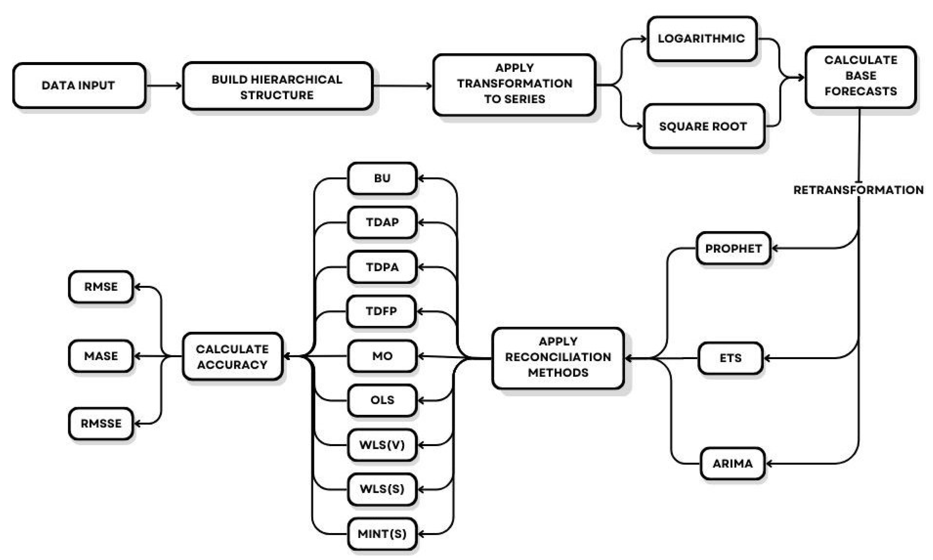
2.7. Flowchart of Methodology

To better understand the methodology used in this study, a flowchart is presented in Figure 3.

3. Empirical Study

3.1. Fire Spots in Brazilian Biomes and Municipalities

A fire spot, also known as a heat spot, is a point with a temperature above 47 °C that may indicate fires or burns. Moreover, flames can originate from one or more locations. A spot is detected by monitoring satellites at approximately 700 to 900 km altitude.
In this study, a hierarchical time series with three levels was considered. Level 0 represents Brazil’s total number of fire spots from January 2011 to December 2022. Level 1 consists of fire spots disaggregated by Brazilian biome: Amazon, Caatinga, Cerrado, Atlantic Forest, Pampa, and Pantanal. The lowest level, or level 2, represents biomes disaggregated by municipality in Brazil, totaling 5570 municipalities. Thus, a total of 5577 time series are included in the hierarchy.
Table 1 presents the descriptive measures of the number of fire spots in Brazil, its biomes, and municipalities. The data show high variability in monthly fire spots across all hierarchy levels, particularly in the municipalities. The Amazon and Cerrado biomes exhibit the highest numbers of fire spots, with significant variability between months, while the Pampa biome has the lowest number of fire spots and the least variability in the data. When grouped by their predominant biome, municipalities generally show a prevalence of months with few or no fire spots; 75% of the total observations from municipalities where the Caatinga, Atlantic Forest, and Pampa are the predominant biomes reported zero fire spots.
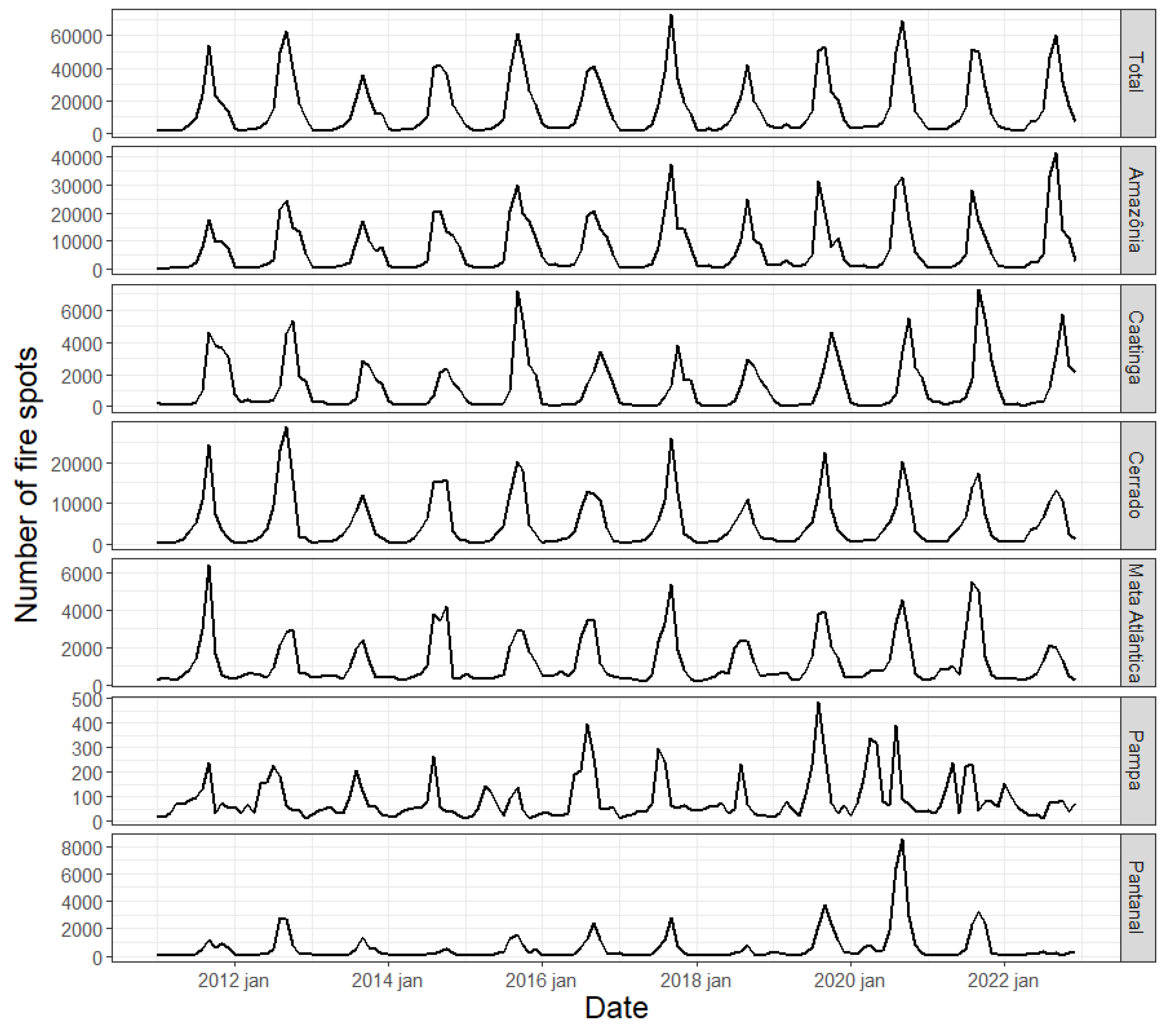
Figure 4 displays the time series of fire spots in Brazil and its biomes, representing the series at levels 0 and 1 of the hierarchy. In 2017, Brazil experienced the month with the highest number of fire spots between 2011 and 2022, with over 60 thousand fire spots. The Amazon had the highest number of fire spots among the six biomes, while the Pampa had the lowest. The sudden increase in the number of spots in the Pantanal in 2020 is noteworthy, a year in which the biome lost approximately 30% of its vegetation [1]. The seasonal component in the series is visible in Figure 4, being less explicit for the Pantanal due to the peak in spots in 2020 and the Pampa, which does not exhibit a well-defined pattern.
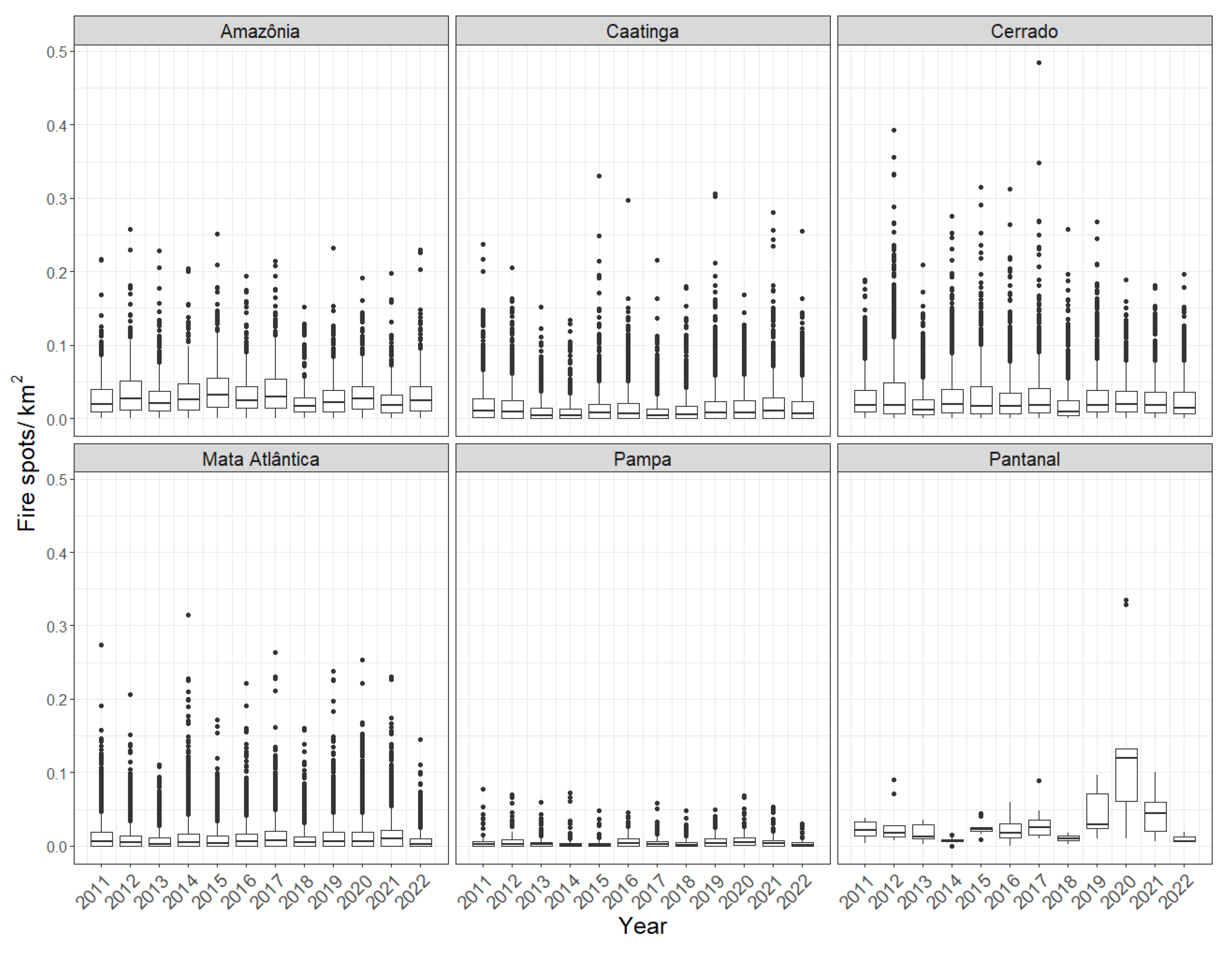
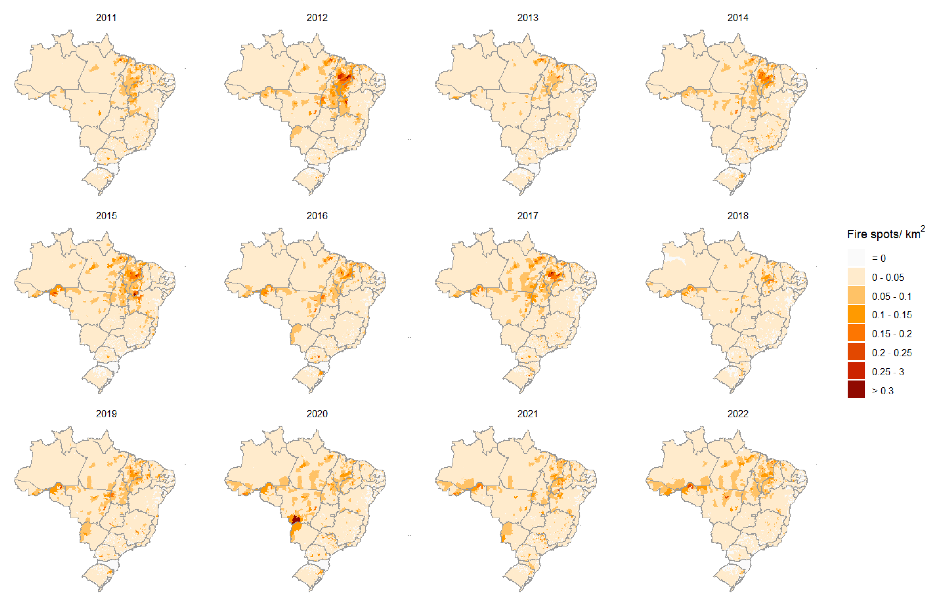
Due to the large number of municipalities (5570), it is unfeasible to visualize the series at the last level of the hierarchy. To better understand the distribution of fire spots and consider the discrepancy in the number of spots between municipalities, analyses were conducted regarding the number of spots per area (km   2 ) from 2011 to 2022 in each municipality (Figure 5, Figure 6, Figure 7 and Figure 8). Most municipalities showed a low number of spots per area. There is no clear trend of increase or decrease in spots over the years (Figure 5 and Figure 6). In the Pantanal, the peak of fires in 2020 is again visible in this graph, and only two municipalities were responsible for most spots in the biome that year (Figure 6). Figure 6 shows that fire spots are not evenly distributed across the country; some municipalities are responsible for most spots in Brazil. From 2011 to 2022, the country’s southern region had few fire spots per km   2 , and the state of Santa Catarina, belonging to this region, had no spots in some years. Municipalities in the states of Maranhão and Tocantins had a high number of spots per km   2 throughout all years. These states have the Cerrado biome as their predominant biome.
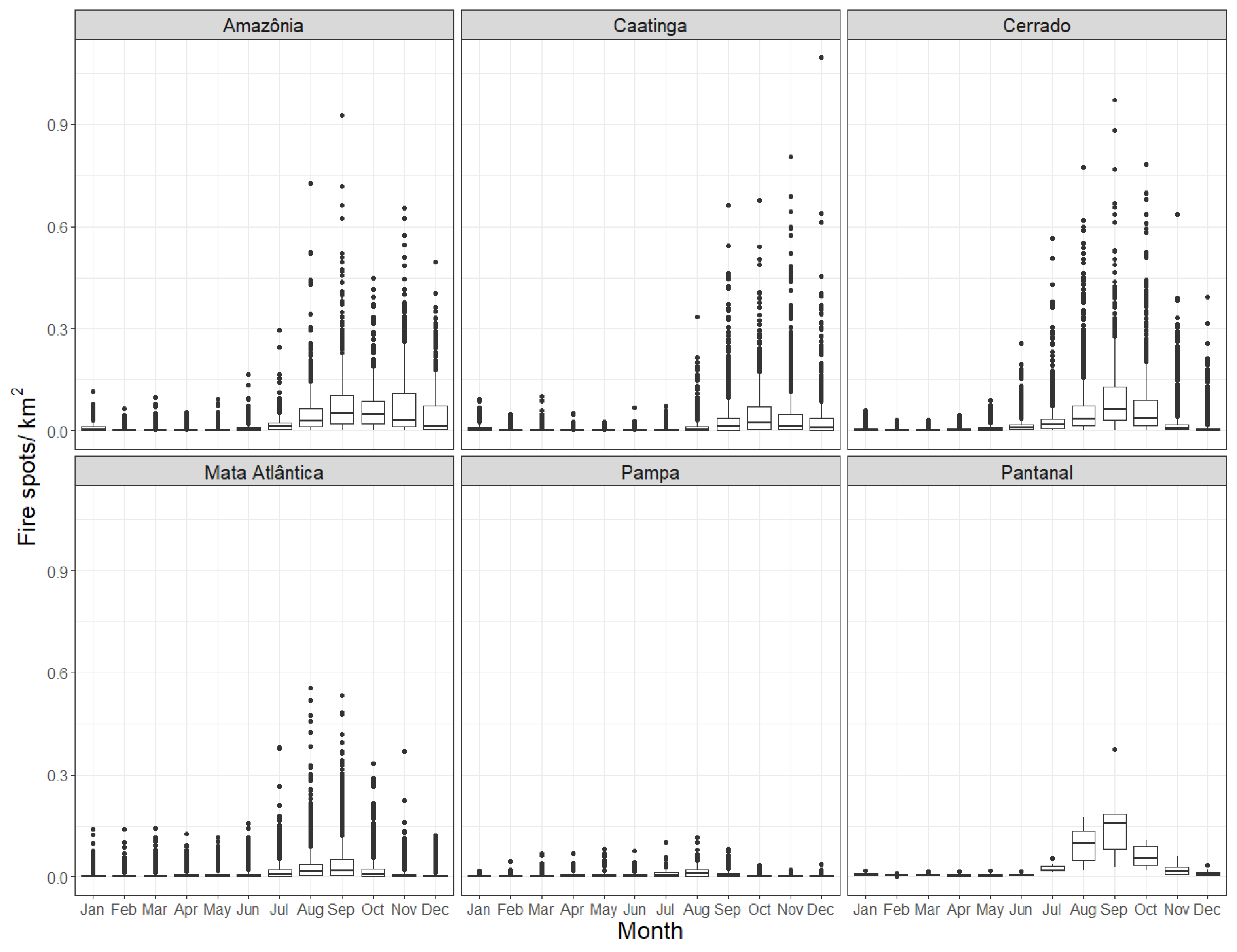
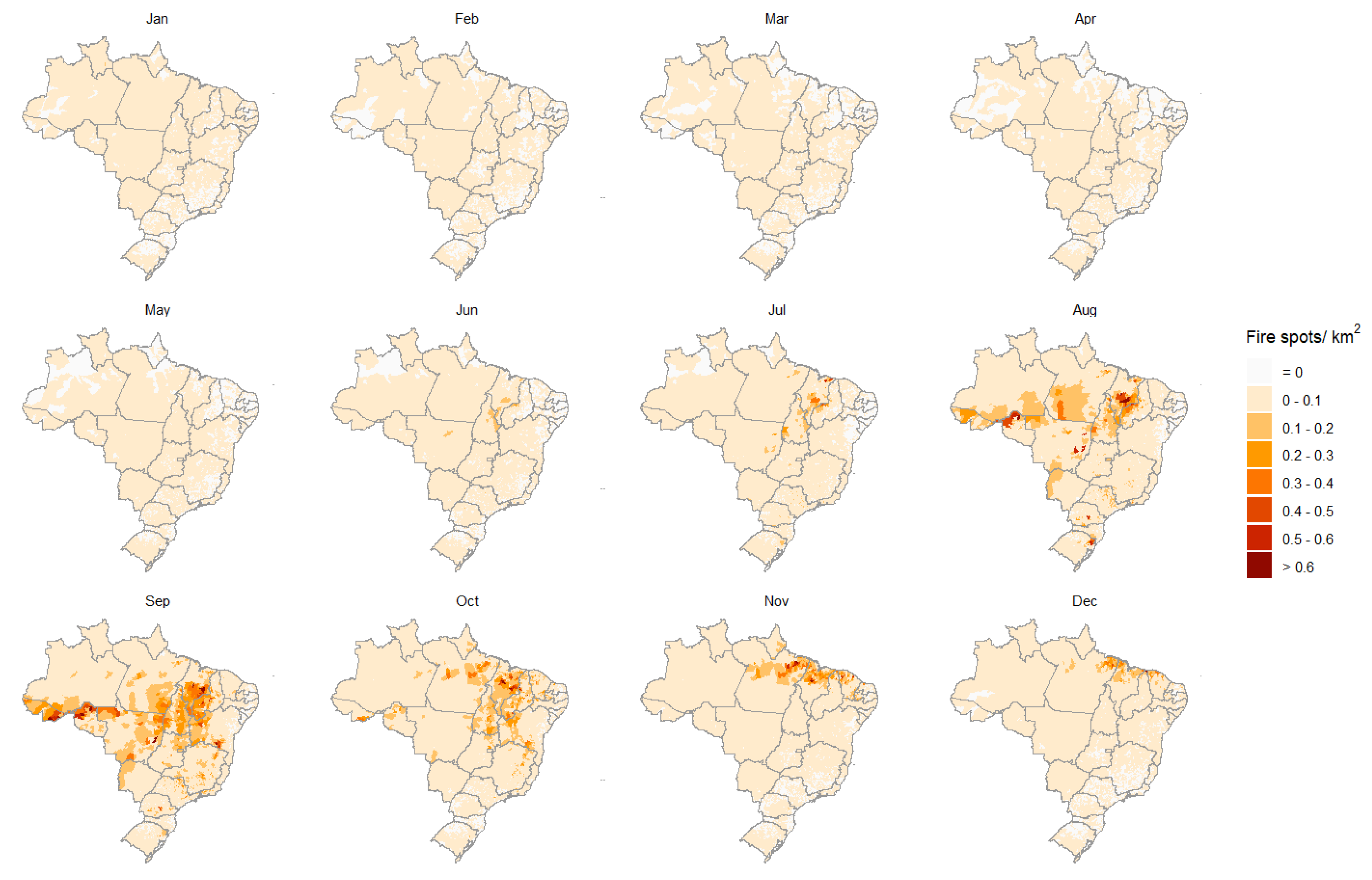
The analysis of the distribution of fire spots per area in each municipality throughout the months of the year indicates the presence of seasonality in the data (Figure 7 and Figure 8). At the beginning of the year, the number of fire spots per area in municipalities is low or zero, and this number begins to increase in July (Figure 7 and Figure 8). The peak of fire spots occurs between September and October, depending on the municipality’s biome. Only in cities where the Pampa is the predominant biome is a pattern less clear to identify (Figure 7). In September, the highest number of fire spots per km   2 occurs throughout the country, and by December, this number decreases considerably (Figure 8). Fires are more frequent in the winter and spring months, from the end of June to the end of December, due to low rainfall levels [30].

3.2. Hierarchical Time Series Forecasting

The routines for calculating fire spot forecasts for the twelve months of 2022 were implemented using R software, version 4.3.0. The results in this section pertain to reconciled forecasts using the square root transformation of fire spots plus 0.5 and the logarithmic transformation of fire spots plus 1. Both transformations used the ARIMA model for base forecasts. The ETS model was also used for base forecasts with the square root transformation of fire spots plus 1. Reconciled forecasts using ETS and the logarithmic transformation of fire spots encountered convergence errors, and the adjusted values and forecasts were unrealistic, so they were not presented.
Table 2 shows the root mean squared error (RMSE) for the level 0 series, related to the overall number of fire spots throughout Brazil, and the average RMSEs for the level 1 and 2 series. Values in bold indicate the lowest RMSEs at each hierarchical level. The results of the average accuracy for different reconciliation approaches using the square root plus 0.5 transformation in the data and the ARIMA model for base forecasts are presented in the first part of the table. With this setup, at level 0, the OLS approach exhibited the lowest RMSE. At level 1, the WLS(s) approach yielded better results, followed by the MinT(s) approach. At level 2, the MinT(s) and WLS(s) outperformed the other approaches. When considering the ARIMA model for base forecasts and a logarithmic transformation of the number of fire spots plus 1, at level 0, the MinT(s) approach had the lowest RMSE. At levels 1 and 2, BU, MinT(s), and WLS(v) outperformed the others (Table 2). The logarithmic transformation results outperformed those based on the square root transformation when the ARIMA model obtained the base forecasts, especially for BU, MinT(s), and WLS(v). When considering the square root transformation and the ETS model to obtain the base forecasts, BU showed better results at level 0, and MinT(s) at the other two levels. The average RMSE values were generally higher than those obtained using the ARIMA model to obtain the base forecasts (Table 2). Reconciled forecasts using ETS and the logarithmic transformation encountered convergence errors, and the adjusted values and forecasts were unrealistic, so they were not presented. When considering the Prophet to obtain the base forecasts, the overall best performance was obtained by BU, followed by MinT(s) and WLS(v) for both transformations (Table 2).
Table 3 is similar to Table 2, but uses MASE as the accuracy measure. The ARIMA model with logarithmic transformation presented the lowest average MASE values, particularly with the MinT(s) approach for level 0 and WLS(v) for levels 1 and 2. Comparing the average MASEs by hierarchical level, level 0, representing Brazil, showed the best results in terms of accuracy, followed by level 1. The MASE values for municipalities were, on average, greater than 1 for all models and approaches.
Table 4 presents the results for the RMSSE, which are similar to those of RMSE and MASE (Table 2 and Table 3) in terms of the best model and approach. Unlike for MASE (Table 3), at level 2, the average RMSSE was less than one for some approaches. The base forecasts without considering any hierarchical structure, especially at levels 0 and 1, resulted in worse outcomes when compared to some reconciliation approaches (Table 2, Table 3 and Table 4).
In addition to calculating the RMSE, MASE, and RMSSE, it is important to know which approaches produce better forecasts than the baseline. If they are not better, hierarchical time series forecasting loses relevance. Table A1, Table A2 and Table A3 of Appendix A show the AveRelRMSE, AveRelMASE, and AveRelRMSSE, respectively, for each level of the hierarchy considering the ARIMA, ETS, and Prophet base forecast models and the two transformations. A value of the AvgRelRMSE, AveRelMASE, and AveRelRMSSE equal to one indicates that the reconciled forecast is equal to the base forecast at that level. An example is the bottom-up approach, which uses base forecasts from municipalities, level 2, and sums them to obtain forecasts for the above levels. A value of AveRelRMSE, AveRelMASE, and AveRelRMSSE lower than one indicates that the reconciled forecasts showed improvements compared to the base forecasts, with bold values being the lowest in Table A1, Table A2 and Table A3.
Here, we summarize the results for the AveRelRMSE (Table A1 of the Appendix A). The interpretation for the AveRelMASE (Table A2 of the Appendix A) and AveRelRMSSE (Table A3 of the Appendix A) are done similarly.
Considering the ARIMA model and the square root transformation of fire spots plus 0.5, at level 0, only the OLS and MO approaches had a value of less than one, showing an improvement of 11.1% and 5.0%, respectively, in RMSE compared to the base forecasts. At level 1, WLS(s) was the one that showed a higher improvement, with a value of 5.8%. At level 2, TDFP showed an improvement of 5.3%. Considering the ARIMA model and the logarithmic transformation of fire spots plus 1, at level 0, only the forecasts from the BU and WLS(v) approaches did not show improvements in the RMSE compared to the base forecasts. At this level, MinT(s) obtained the best result, with an improvement of 22.2% in the RMSE value. At level 1, out of the nine approaches, four of them showed improvements in the RMSE up to 20.0%. In the last level, no method showed improvement compared to the base forecasts (Table A1). When considering the Prophet model for the base forecasts, the overall best reconciliation method was the BU, but without an RMSE improvement in level two. Overall, the MinT(s) and TDFP approaches outperformed the remaining when considering the logarithm transformation and the ARIMA model to obtain the base forecasts.
The AvgRelRMSE of the approaches using ETS for base forecasts and the square root transformation of fire spots plus 0.5 is also presented in Table A1. At level 0, excluding the top-down approaches that use base forecasts at this level, all approaches showed improvements in RMSE. BU showed an improvement of 76.3% at this level. At level 1, only WLS(s) and TDPA showed improvements in RMSE, and six approaches showed improvements in RMSE at level 2, with TDPA having the highest improvement. It is also noted that the MO and TDPA approaches showed improvements at all levels.
When considering the Prophet model for the base forecasts, the most effective reconciliation method overall was the BU, except for level 0 in the case of the square root transformation, where the TDPA showed superior performance.
Despite the percentage improvements in RMSE, it is important to consider that the reconciled forecasts using each base model and transformation have different magnitudes. For example, the ETS model with the square root transformation had the overall highest RMSE values (Table 2) compared to the prophet with the logarithm transformation. Thus, reconciled forecasts using the ETS model show significant improvements over base forecasts, but they are not better than those using the Prophet model.
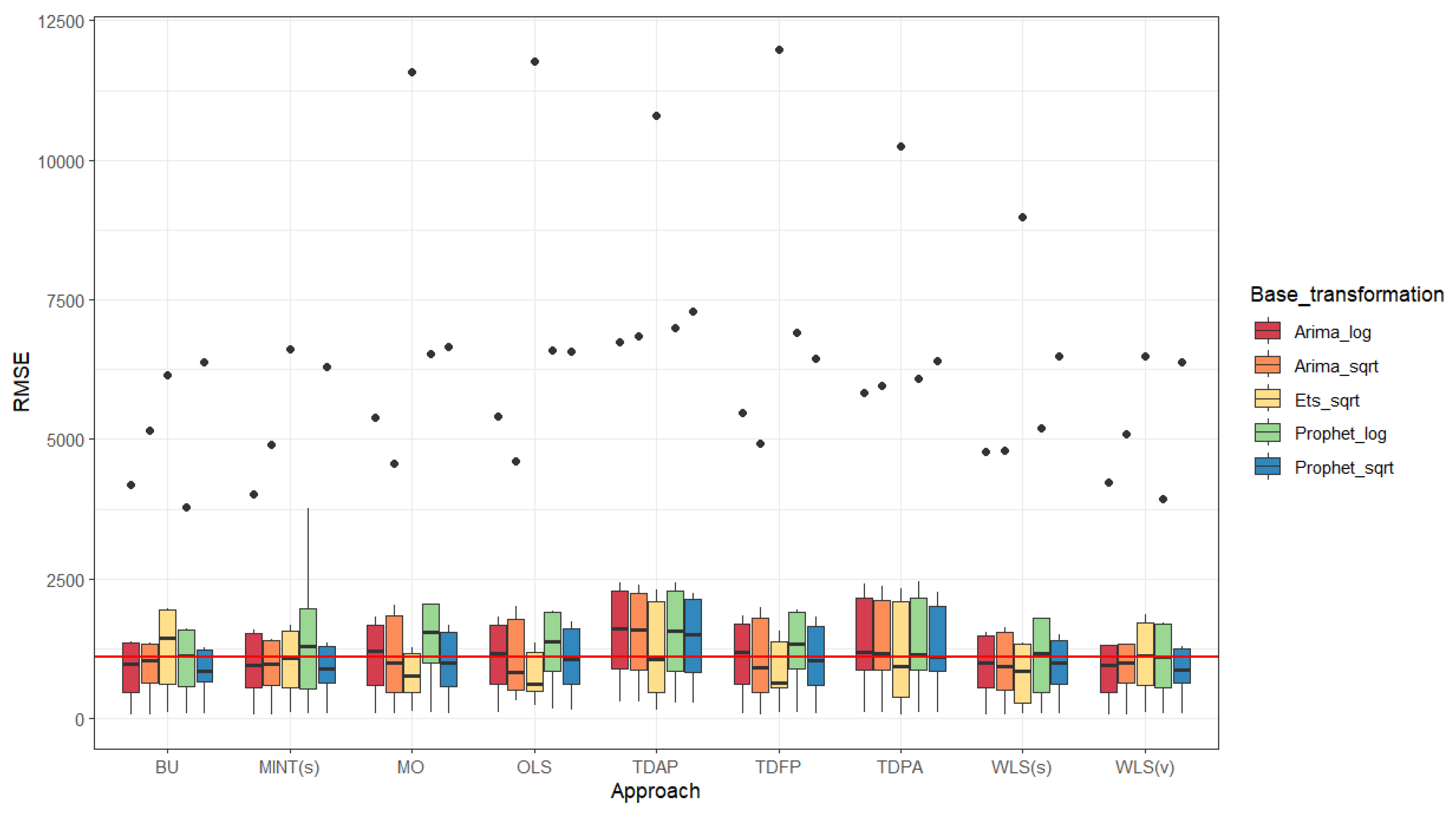
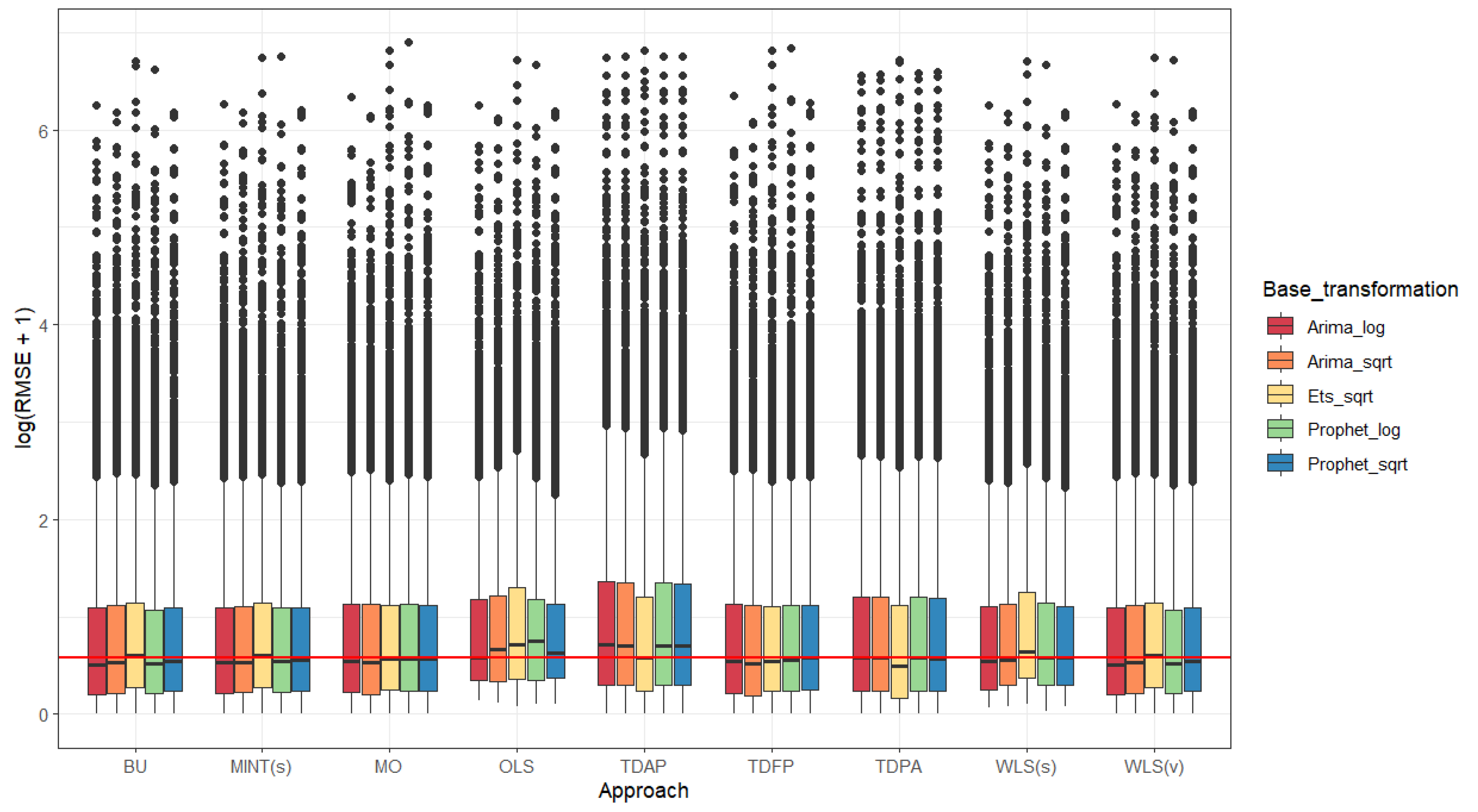
Figure 9 and Figure 10 show the boxplots for the RMSE for the nine forecasting reconciliation approaches and the three models and two transformations under consideration for level one (biomes) and level two (municipalities), respectively. For level one (Figure 9), the WLS(s) seems to be the better-performing reconciliation approach, and the ETS model with the square root transformation is the best to obtain the base forecasts. For level two (Figure 10), when not considering the “outliers”, a good overall performance was obtained for the TDFP reconciliation approach, and the ETS with the square root transformation seems to be the overall winner in performance.
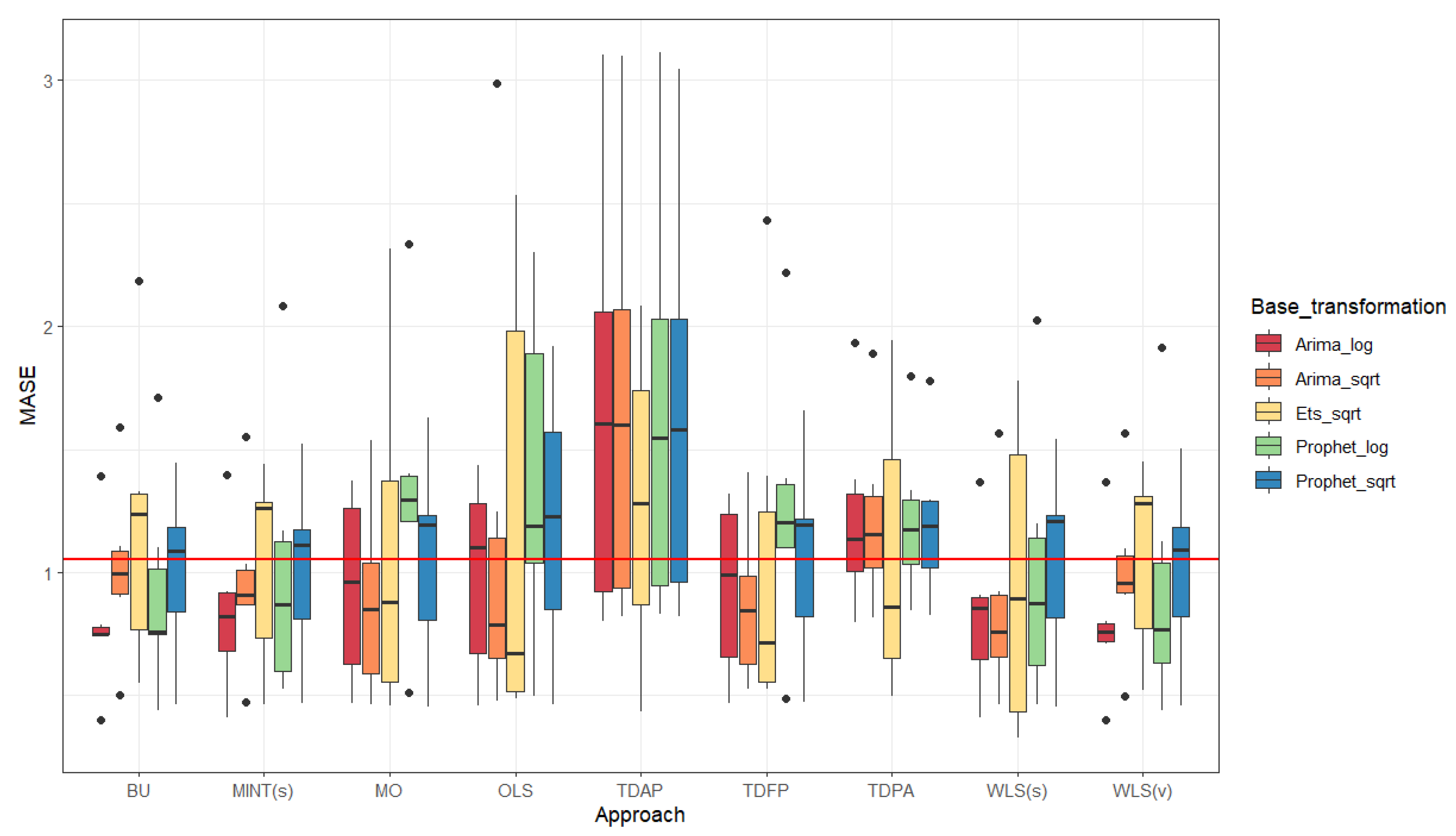
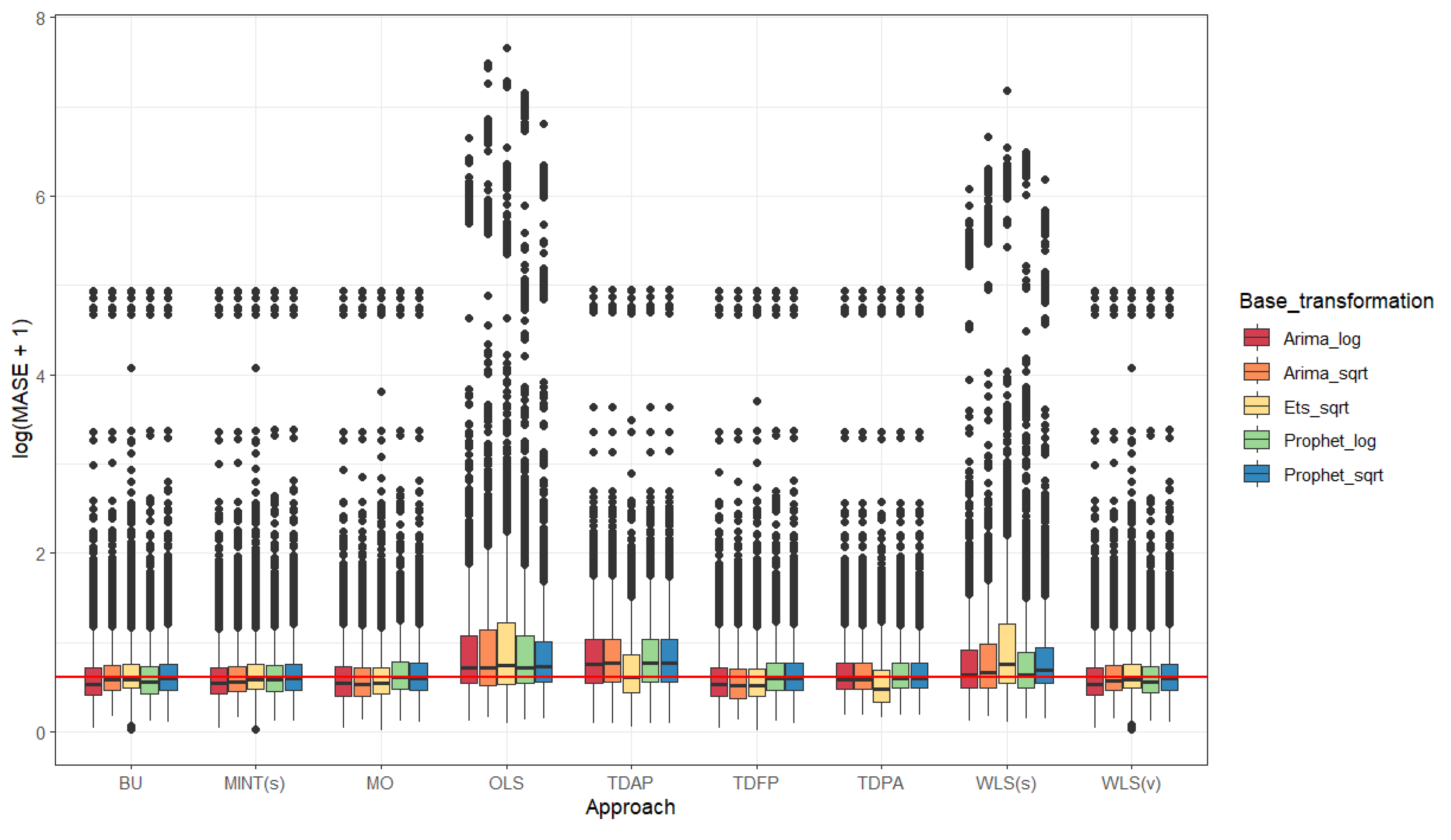
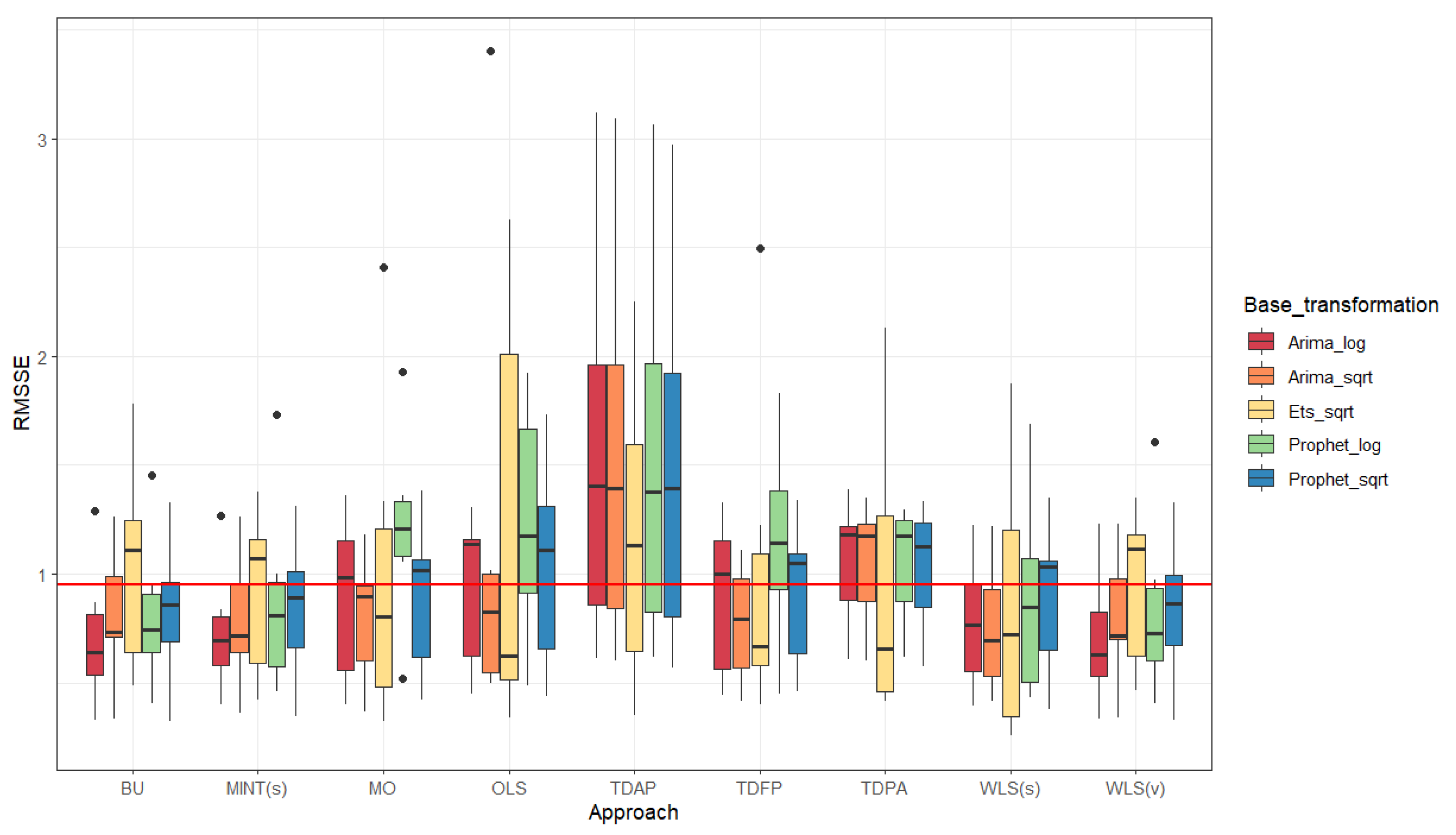
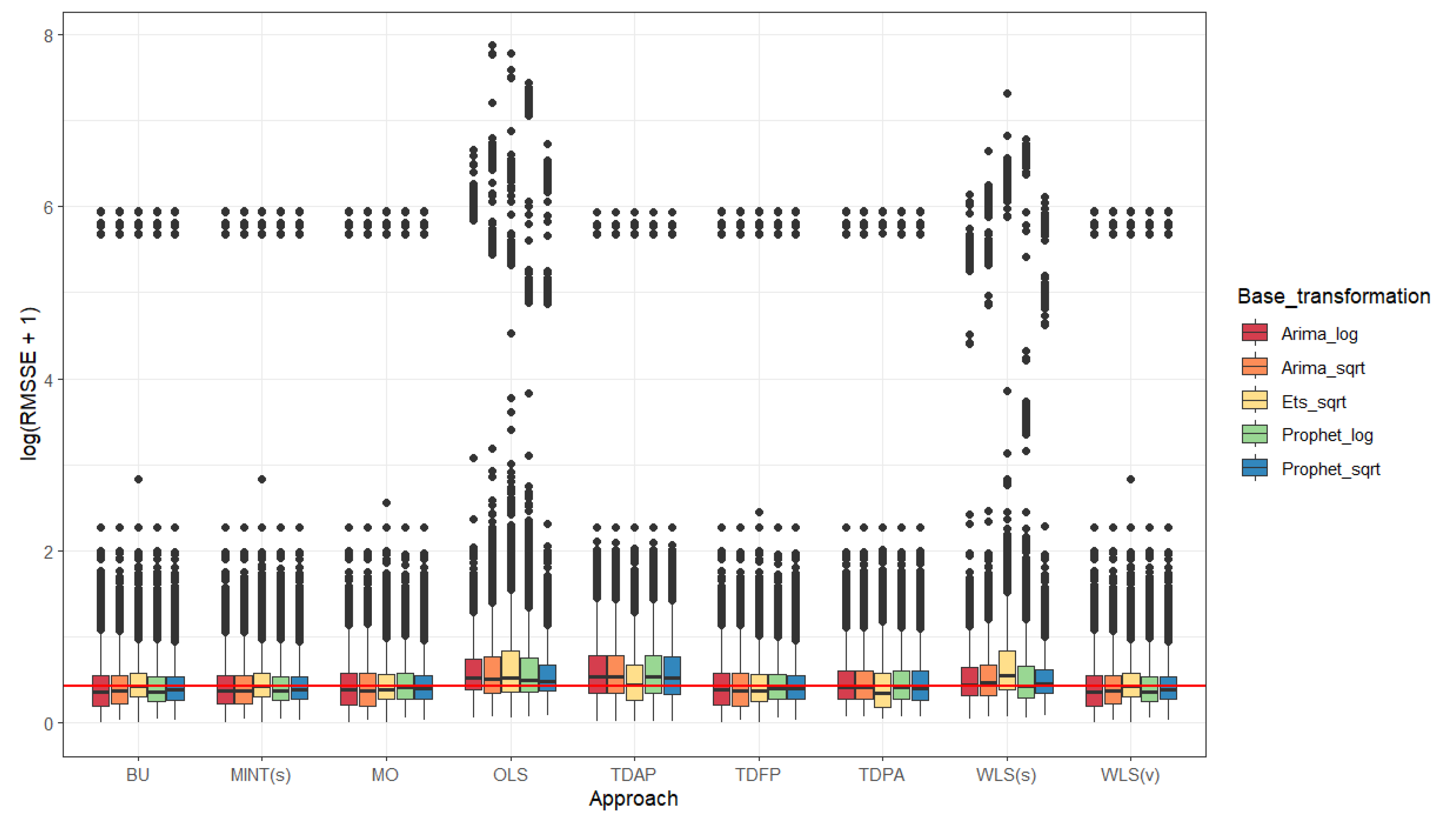
Figure A1 and Figure A2 show the boxplots for the MASE for the nine forecasting reconciliation approaches and the three models and two transformations under consideration for level one (biomes) and level two (municipalities), respectively. Figure A3 and Figure A4 show the boxplots for the RMSSE for the nine forecasting reconciliation approaches and the three models and two transformations under consideration for level one (biomes) and level two (municipalities), respectively. The overall conclusions from Table A1, Table A2 and Table A3 are in the same line as those for the RMSE (Figure 9 and Figure 10).

4. Concluding Remarks

In this study, we comprehensively analyzed various reconciliation approaches to forecasting the number of fire spots, considering different base forecast models and data transformations. The results offer valuable insights into the effectiveness of these approaches at different hierarchical levels, ranging from biomes to municipalities.
Our findings indicate that the choice of the reconciliation method is crucial and depends on factors such as the base forecasting model and the transformation applied to the data. At level 0, the bottom-up (BU) approach demonstrated stronger performance, particularly when using the Prophet model and the logarithm transformation. However, alternative methods, such as WLS, BU, and MinT, exhibited competitive results at other levels.
Moreover, the influence of data transformations, including square root and logarithmic transformations, was evident in the performance of reconciliation approaches. Notably, when combined with the ARIMA or the Prophet model, the logarithmic transformation showcased superior results for certain approaches at various levels.
The AveRelRMSE, AveRelMASE, and AveRelRMSSE metrics provided a nuanced understanding of the improvements achieved by each reconciliation approach compared to baseline forecasts. This information is essential for practical decision-making, emphasizing the importance of not only minimizing forecast errors but also ensuring improvements over the baseline.
It is worth noting that the reconciliation methods exhibited diverse performance across different levels of the hierarchical structure, suggesting the need for adaptive strategies based on the specific forecasting context.
In summary, this study contributes valuable insights into applying forecasting reconciliation in fire spot forecasts. The results presented here guide practitioners and decision-makers in choosing reconciliation methods tailored to their specific forecasting scenarios. As the field continues to evolve, future research may explore additional factors influencing reconciliation effectiveness and expand the applicability of these findings to diverse domains.

Author Contributions

Conceptualization, P.C.R.; methodology, A.C.P. and P.C.R.; software, A.C.P.; validation, A.C.P. and P.C.R.; formal analysis, A.C.P. and P.C.R.; investigation, A.C.P. and P.C.R.; writing—original draft preparation, A.C.P. and P.C.R.; writing—review and editing, A.C.P. and P.C.R.; visualization, A.C.P.; supervision, P.C.R. All authors have read and agreed to the published version of the manuscript.

Funding

This research received no external funding.

Institutional Review Board Statement

Not applicable.

Informed Consent Statement

Not applicable.

Data Availability Statement

The data are available in https://github.com/SaLLy-laboratory/HTS-Brazilian-firesopts (accessed on 26 June 2024).

Conflicts of Interest

The authors declare no conflicts of interest.

Appendix A

Table A1. AveRelRMSE per hierarchical level using (i) the square root transformation and the ARIMA model for base forecasts; (ii) the logarithmic transformation and the ARIMA model for base forecasts; (iii) the square root transformation and the ETS model for base forecasts; (iv) the square root transformation and the Prophet model for base forecasts; and (v) the logarithmic transformation and the Prophet model for base forecasts.
BUMinT(s)MOOLSTDAPTDFPTDPAWLS(s)WLS(v)
ARIMA–Square root transformation
Level 01.8301.3000.9500.8901.0001.0001.0001.0161.749
Level 11.0030.9751.0001.2261.7710.9811.3640.9420.990
Level 21.0001.0010.9751.9131.5860.9471.2081.6420.999
ARIMA–Logarithm transformation
Level 01.1670.7780.9970.9891.0001.0001.0001.0021.173
Level 10.8040.8591.0001.0661.6451.0191.2660.8920.800
Level 21.0001.0711.0662.2641.8251.0551.3901.8051.001
ETS–Square root transformation
Level 00.2370.3010.8810.9811.0001.0001.0000.6660.272
Level 11.1781.0501.0001.0871.2381.0300.9830.8351.095
Level 21.0000.9940.9141.6760.9520.8760.7571.7110.999
Prophet–Square root transformation
Level 01.4061.2921.1391.0141.0191.0110.9861.1651.376
Level 10.9250.9401.0001.1271.5421.0241.1930.9910.928
Level 21.0001.0071.0311.5931.3781.0391.0531.4501.000
Prophet–Logarithm transformation
Level 00.5760.8670.9830.9581.0051.0020.9870.8040.596
Level 10.6710.7091.0000.9911.1600.9300.8980.6990.673
Level 21.0001.0351.1321.8571.4761.1011.1261.3971.001
Table A2. AveRelMASE per hierarchical level using (i) the square root transformation and the ARIMA model for base forecasts; (ii) the logarithmic transformation and the ARIMA model for base forecasts; (iii) the square root transformation and the ETS model for base forecasts; (iv) the square root transformation and the Prophet model for base forecasts; and (v) the logarithmic transformation and the Prophet model for base forecasts.
BUMinT(s)MOOLSTDAPTDFPTDPAWLS(s)WLS(v)
ARIMA–Square root transformation
Level 01.8581.3051.0780.9221.0001.0001.0001.0131.769
Level 11.1811.1111.0001.1541.8331.0101.4560.9751.162
Level 21.0000.9650.8861.7461.3510.8421.0361.4970.999
ARIMA–Logarithm transformation
Level 01.1810.8320.9360.9681.0001.0001.0000.9561.177
Level 10.8700.9061.0001.0571.7061.0071.3570.8960.866
Level 21.0001.0411.0032.0401.6160.9871.2391.6531.001
ETS–Square root transformation
Level 00.2710.3040.8550.9771.0001.0001.0000.6580.294
Level 11.1751.0491.0001.0171.2370.9671.0280.8641.093
Level 21.0000.9920.8911.7680.9610.8440.7571.7980.999
Prophet–Square root transformation
Level 01.3481.2551.0661.0021.0191.0030.9901.1201.326
Level 10.9680.9721.0001.1081.5131.0111.2000.9940.970
Level 21.0001.0041.0001.6011.3661.0051.0491.4541.000
Prophet–Logarithm transformation
Level 00.6461.0431.0560.9710.9980.9880.9820.8650.698
Level 10.6880.7341.0021.0021.2100.9430.9690.7240.680
Level 21.0001.0481.1161.8421.4801.0841.1361.4151.002
Table A3. AveRelRMSSE per hierarchical level using (i) the square root transformation and the ARIMA model for base forecasts; (ii) the logarithmic transformation and the ARIMA model for base forecasts; (iii) the square root transformation and the ETS model for base forecasts; (iv) the square root transformation and the Prophet model for base forecasts; and (v) the logarithmic transformation and the Prophet model for base forecasts.
BUMinT(s)MOOLSTDAPTDFPTDPAWLS(s)WLS(v)
ARIMA–Square root transformation
Level 01.8301.3000.9500.8901.0001.0001.0001.0161.749
Level 11.0030.9751.0001.2261.7710.9811.3640.9420.990
Level 21.0001.0010.9751.9131.5860.9471.2081.6420.999
ARIMA–Logarithm transformation
Level 01.1670.7780.9970.9891.0001.0001.0001.0021.173
Level 10.8040.8591.0001.0661.6451.0191.2660.8920.800
Level 21.0001.0711.0662.2641.8251.0551.3901.8051.001
ETS–Square root transformation
Level 00.2370.3010.8810.9811.0001.0001.0000.6660.272
Level 11.1781.0501.0001.0871.2381.0300.9830.8351.095
Level 21.0000.9940.9141.6760.9520.8760.7571.7110.999
Prophet–Square root transformation
Level 01.4061.2921.1391.0141.0191.0110.9861.1651.376
Level 10.9250.9401.0001.1271.5421.0241.1930.9910.928
Level 21.0001.0071.0311.5931.3781.0391.0531.4501.000
Prophet–Logarithm transformation
Level 00.5760.8670.9830.9581.0051.0020.9870.8040.596
Level 10.6710.7091.0000.9911.1600.9300.8980.6990.673
Level 21.0001.0351.1321.8571.4761.1011.1261.3971.001

Appendix B

Figure A1. Boxplots for the mean absolute scaled error for 12 ahead forecast of the number of fire spots for all six Brazilian biomes considering the nine forecasting reconciliation approaches, using (i) the square root transformation and the ARIMA model for base forecasts; and (ii) the logarithmic transformation and the ARIMA model for base forecasts; (iii) the square root transformation and the ETS model for base forecasts; (iv) the square root transformation and the Prophet model for base forecasts; and (v) the logarithmic transformation and the Prophet model for base forecasts; red line: mean of the medians.
Stats 07 00039 g0a1
Figure A2. Boxplots for the mean absolute scaled error for 12 ahead forecast of the number of fire spots for all 5570 Brazilian municipalities considering the nine forecasting reconciliation approaches, using (i) the square root transformation and the ARIMA model for base forecasts; and (ii) the logarithmic transformation and the ARIMA model for base forecasts; (iii) the square root transformation and the ETS model for base forecasts; (iv) the square root transformation and the Prophet model for base forecasts; and (v) the logarithmic transformation and the Prophet model for base forecasts; red line: mean of the medians.
Stats 07 00039 g0a2
Figure A3. Boxplots for the root mean squared scaled error for 12 ahead forecast of the number of fire spots for all six Brazilian biomes considering the nine forecasting reconciliation approaches, using (i) the square root transformation and the ARIMA model for base forecasts; and (ii) the logarithmic transformation and the ARIMA model for base forecasts; (iii) the square root transformation and the ETS model for base forecasts; (iv) the square root transformation and the Prophet model for base forecasts; and (v) the logarithmic transformation and the Prophet model for base forecasts; red line: mean of the medians.
Stats 07 00039 g0a3
Figure A4. Boxplots for the root mean squared scaled error for 12 ahead forecast of the number of fire spots for all 5570 Brazilian municipalities considering the nine forecasting reconciliation approaches, using (i) the square root transformation and the ARIMA model for base forecasts; and (ii) the logarithmic transformation and the ARIMA model for base forecasts; (iii) the square root transformation and the ETS model for base forecasts; (iv) the square root transformation and the Prophet model for base forecasts; and (v) the logarithmic transformation and the Prophet model for base forecasts; red line: mean of the medians.
Stats 07 00039 g0a4

References

  1. Pivello, V.R.; Vieira, I.; Christianini, A.V.; Ribeiro, D.B.; da Silva Menezes, L.; Berlinck, C.N.; Melo, F.P.; Marengo, J.A.; Tornquist, C.G.; Tomas, W.M.; et al. Understanding Brazil’s catastrophic fires: Causes, consequences and policy needed to prevent future tragedies. Perspect. Ecol. Conserv. 2021, 19, 233–255. [Google Scholar] [CrossRef]
  2. Butt, E.W.; Conibear, L.; Knote, C.; Spracklen, D.V. Large air quality and public health impacts due to Amazonian deforestation fires in 2019. GeoHealth 2021, 5, e2021GH000429. [Google Scholar] [CrossRef] [PubMed]
  3. Morello, T.F.; Ramos, R.M.; Anderson, L.O.; Owen, N.; Rosan, T.M.; Steil, L. Predicting fires for policy making: Improving accuracy of fire brigade allocation in the Brazilian Amazon. Ecol. Econ. 2020, 169, 106501. [Google Scholar] [CrossRef]
  4. Viganó, H.H.D.G.; Souza, C.C.D.; Reis Neto, J.F.; Cristaldo, M.F.; Jesus, L.D. Prediction and modeling of forest fires in the Pantanal. Rev. Bras. Meteorol. 2018, 33, 306–316. [Google Scholar] [CrossRef]
  5. Gama Viganó, H.H.; de Souza, C.C.; Cristaldo, M.F.; de Jesus, L. Redes neurais artificiais na previsão de queimadas e incêndios no Pantanal. Rev. Bras. Geogr. Física 2017, 10, 1355–1367. [Google Scholar] [CrossRef]
  6. Hyndman, R.J.; Ahmed, R.A.; Athanasopoulos, G.; Shang, H.L. Optimal combination forecasts for hierarchical time series. Comput. Stat. Data Anal. 2011, 55, 2579–2589. [Google Scholar] [CrossRef]
  7. Lila, M.F.; Meira, E.; Oliveira, F.L.C. Forecasting unemployment in Brazil: A robust reconciliation approach using hierarchical data. Socio-Econ. Plan. Sci. 2022, 82, 101298. [Google Scholar] [CrossRef]
  8. Gaweł, B.; Paliński, A. Global and Local Approaches for Forecasting of Long-Term Natural Gas Consumption in Poland Based on Hierarchical Short Time Series. Energies 2024, 17, 347. [Google Scholar] [CrossRef]
  9. Wickramasuriya, S.L.; Athanasopoulos, G.; Hyndman, R.J. Optimal forecast reconciliation for hierarchical and grouped time series through trace minimization. J. Am. Stat. Assoc. 2019, 114, 804–819. [Google Scholar] [CrossRef]
  10. Athanasopoulos, G.; Hyndman, R.J.; Kourentzes, N.; Panagiotelis, A. Forecast reconciliation: A review. Int. J. Forecast. 2023, 40, 430–456. [Google Scholar] [CrossRef]
  11. Hollyman, R.; Petropoulos, F.; Tipping, M.E. Understanding forecast reconciliation. Eur. J. Oper. Res. 2021, 294, 149–160. [Google Scholar] [CrossRef]
  12. Winters, P.R. Forecasting sales by exponentially weighted moving averages. Manag. Sci. 1960, 6, 324–342. [Google Scholar] [CrossRef]
  13. Holt, C. Forecasting Seasonals and Trends by Exponentially Weighted Averages (ONR Memorandum No. 52); Carnegie Institute of Technology: Pittsburgh, PA, USA, 1957; Volume 10. [Google Scholar]
  14. Sulandari, W.; Suhartono; Subanar; Rodrigues, P. C. Exponential smoothing on modeling and forecasting multiple seasonal time series: An overview. Fluct. Noise Lett. 2021, 20, 2130003. [Google Scholar] [CrossRef]
  15. Taylor, S.J.; Letham, B. Forecasting at scale. Am. Stat. 2018, 72, 37–45. [Google Scholar] [CrossRef]
  16. Pimentel, J.; Bulhões, R.; Rodrigues, P.C. Spatio-temporal modeling of the Brazilian wildfires: The influence of human and meteorological variables. In Proceedings of the 64th ISI World Statistics Congress, Ottawa, ON, Canada, 16–20 July 2023. [Google Scholar]
  17. da Silva, G.; Fasiaben, M.; Nogueira, S.; Grego, C.; Moraes, A.; Almeida, M.; de Oliveira, O.; Eusebio, G.; Lopes, W. Método Para Determinar o Bioma Predominante nos Municípios Brasileiros; Embrapa Agricultura Digital: Campinas, Brazil, 2022. [Google Scholar]
  18. Gross, C.W.; Sohl, J.E. Disaggregation methods to expedite product line forecasting. J. Forecast. 1990, 9, 233–254. [Google Scholar] [CrossRef]
  19. Athanasopoulos, G.; Ahmed, R.A.; Hyndman, R.J. Hierarchical forecasts for Australian domestic tourism. Int. J. Forecast. 2009, 25, 146–166. [Google Scholar] [CrossRef]
  20. Hyndman, R.J.; Lee, A.J.; Wang, E. Fast computation of reconciled forecasts for hierarchical and grouped time series. Comput. Stat. Data Anal. 2016, 97, 16–32. [Google Scholar] [CrossRef]
  21. Athanasopoulos, G.; Hyndman, R.J.; Kourentzes, N.; Petropoulos, F. Forecasting with temporal hierarchies. Eur. J. Oper. Res. 2017, 262, 60–74. [Google Scholar] [CrossRef]
  22. Schäfer, J.; Strimmer, K. A shrinkage approach to large-scale covariance matrix estimation and implications for functional genomics. Stat. Appl. Genet. Mol. Biol. 2005, 4, 1–32. [Google Scholar] [CrossRef] [PubMed]
  23. Box, G.E.; Jenkins, G.M.; Reinsel, G.C.; Ljung, G.M. Time Series Analysis: Forecasting and Control; John Wiley & Sons: Hoboken, NJ, USA, 2015. [Google Scholar]
  24. Hyndman, R.J.; Khandakar, Y. Automatic time series forecasting: The forecast package for R. J. Stat. Softw. 2008, 27, 1–22. [Google Scholar] [CrossRef]
  25. Sugiura, N. Further analysis of the data by Akaike’s information criterion and the finite corrections. Commun. Stat.-Theory Methods 1978, 7, 13–26. [Google Scholar] [CrossRef]
  26. Gardner, E.S., Jr.; McKenzie, E. Forecasting trends in time series. Manag. Sci. 1985, 31, 1237–1246. [Google Scholar] [CrossRef]
  27. Hyndman, R.J.; Koehler, A.B.; Snyder, R.D.; Grose, S. A state space framework for automatic forecasting using exponential smoothing methods. Int. J. Forecast. 2002, 18, 439–454. [Google Scholar] [CrossRef]
  28. Hyndman, R.J.; Koehler, A.B. Another look at measures of forecast accuracy. Int. J. Forecast. 2006, 22, 679–688. [Google Scholar] [CrossRef]
  29. Davydenko, A.; Fildes, R. Measuring forecasting accuracy: The case of judgmental adjustments to SKU-level demand forecasts. Int. J. Forecast. 2013, 29, 510–522. [Google Scholar] [CrossRef]
  30. Pezzopane, J.E.M.; Neto, S.N.D.O.; Vilela, M.D.F. Risco de incêndios em função da característica do clima, relevo e cobertura do solo. Floresta Ambiente 2012, 8, 161–166. [Google Scholar]
Figure 1. Geographic localization of each of the six Brazilian biomes.
Stats 07 00039 g001
Figure 2. A three-level hierarchical tree diagram.
Stats 07 00039 g002
Figure 3. Flowchart of the methodology used in the paper.
Stats 07 00039 g003
Figure 4. Time series of the monthly number of forest fire spots in Brazil and each of the six Brazilian biomes.
Stats 07 00039 g004
Figure 5. Boxplots for the annual number of fire spots in Brazilian municipalities divided by their area and grouped by the municipality’s predominant biome.
Stats 07 00039 g005
Figure 6. Maps of the total fire spots in Brazilian municipalities divided by their area from 2011 to 2022.
Stats 07 00039 g006
Figure 7. Boxplots for the monthly number of fire spots in Brazilian municipalities divided by their area and grouped by the municipality’s predominant biome, considering the years from 2011 to 2022.
Stats 07 00039 g007
Figure 8. Maps of the total forest fire spots in Brazilian municipalities divided by their area per month, considering the years from 2011 to 2022.
Stats 07 00039 g008
Figure 9. Boxplots for the root mean squared error for 12 ahead forecast of the number of fire spots for all six Brazilian biomes considering the nine forecasting reconciliation approaches, using (i) the square root transformation and the ARIMA model for base forecasts; and (ii) the logarithmic transformation and the ARIMA model for base forecasts; (iii) the square root transformation and the ETS model for base forecasts; (iv) the square root transformation and the Prophet model for base forecasts; and (v) the logarithmic transformation and the Prophet model for base forecasts; red line: mean of the medians.
Stats 07 00039 g009
Figure 10. Boxplots for the logarithm of the root mean squared error plus one for 12 ahead forecast of the number of fire spots for all 5570 Brazilian municipalities considering the nine forecasting reconciliation approaches, using (i) the square root transformation and the ARIMA model for base forecasts; and (ii) the logarithmic transformation and the ARIMA model for base forecasts; (iii) the square root transformation and the ETS model for base forecasts; (iv) the square root transformation and the Prophet model for base forecasts; and (v) the logarithmic transformation and the Prophet model for base forecasts red line: mean of the medians.
Stats 07 00039 g010
Table 1. Descriptive measures of the number of fire spots in Brazil, its biomes, and municipalities.
Min1st QuartileMedianMean3rd QuartileMaxSDCV
Brazil11262702.507080.515,351.0620,630.5072,89517,381.45113.23
Biome
Amazônia273922.752517.07277.4911,143.5041,4818962.50123.15
Caatinga25123.75306.51191.621711.7572711579.92132.59
Cerrado233748.502301.05030.307298.0028,5466099.56121.26
Mata Atlântica193377.75573.51190.561541.5064381270.43106.71
Pampa1236.0058.088.2091.7548586.6498.23
Pantanal460.50159.0572.89559.5084971113.68194.40
Municipality
Amazônia00114.477357770.02483.98
Caatinga0001.09012987.65703.67
Cerrado0004.732154021.17447.36
Mata Atlântica0000.4303292.54583.90
Pampa0000.550431.92347.88
Pantanal01663.65312523215.56338.64
Table 2. Average RMSE per hierarchical level using (i) the square root transformation and the ARIMA model for base forecasts; (ii) the logarithmic transformation and the ARIMA model for base forecasts; (iii) the square root transformation and the ETS model for base forecasts; (iv) the square root transformation and the Prophet model for base forecasts; and (v) the logarithmic transformation and the Prophet model for base forecasts.
BaseBUMinT(s)MOOLSTDAPTDFPTDPAWLS(s)WLS(v)
ARIMA–Square root transformation
Level 01945.013559.092527.781848.321731.791945.011945.011945.011976.473401.77
Level 11506.601541.121493.221506.601516.882238.071542.041934.351475.371519.82
Level 23.633.633.613.663.815.593.664.563.693.61
ARIMA–Logarithm transformation
Level 01681.921963.261307.861676.901662.921681.921681.921681.921684.681973.06
Level 11683.261329.781355.901683.261686.892235.391698.421927.021482.961325.33
Level 23.513.513.533.733.735.613.734.573.593.51
ETS–Square root transformation
Level 011,492.092727.343459.9610,122.9611,270.6411,492.0911,492.0911,492.097652.483127.44
Level 12481.411929.941831.772481.412511.182630.492586.162479.502056.691860.50
Level 24.154.154.054.464.885.234.504.644.444.07
Prophet–Square root transformation
Level 03116.494381.064027.543549.053161.253175.723150.093074.123631.564287.71
Level 11816.601685.201693.751819.541853.532255.261821.141967.021768.381689.48
Level 23.693.693.703.803.845.543.804.553.763.70
Prophet–Logarithm transformation
Level 02590.241491.702245.592545.242481.832603.392596.492557.642083.341544.51
Level 12124.871376.001481.082133.442051.942258.142087.701961.761643.811412.05
Level 23.613.613.704.144.115.584.094.563.823.66
Table 3. Average MASE per hierarchical level using (i) the square root transformation and the ARIMA model for base forecasts; (ii) the logarithmic transformation and the ARIMA model for base forecasts; (iii) the square root transformation and the ETS model for base forecasts; (iv) the square root transformation and the Prophet model for base forecasts; and (v) the logarithmic transformation and the Prophet model for base forecasts.
BaseBUMinT(s)MOOLSTDAPTDFPTDPAWLS(s)WLS(v)
ARIMA–Square root transformation
Level 00.2870.5330.3750.3100.2650.2870.2870.2870.2910.508
Level 10.8831.0140.9560.8831.1501.6770.8681.2260.8540.997
Level 21.1411.1411.1101.05215.8891.6171.0171.15910.6131.140
ARIMA–Logarithm transformation
Level 00.2450.2890.2040.2290.2370.2450.2450.2450.2340.289
Level 10.9400.8030.8380.9400.9941.6700.9381.2230.8300.799
Level 21.0431.0431.0571.05311.8461.6141.0421.1577.2501.043
ETS–Square root transformation
Level 01.3950.3770.4251.1921.3631.3951.3951.3950.9170.410
Level 11.0871.1941.0471.0871.2071.2841.0511.0650.9741.075
Level 21.2201.2201.2121.11712.1491.2351.0750.97914.9161.219
Prophet–Square root transformation
Level 00.4390.5920.5510.4680.4400.4480.4400.4350.4920.582
Level 11.0641.0101.0201.0651.2081.6601.0731.2121.0551.016
Level 21.1551.1551.1581.1528.7671.6281.1561.1676.4811.155
Prophet–Logarithm transformation
Level 00.3380.2180.3530.3570.3280.3370.3340.3320.2920.236
Level 11.3390.9191.0111.3411.3801.6621.2651.2191.0000.934
Level 21.0701.0701.1041.16814.0691.6241.1411.1636.7831.071
Table 4. Average RMSSE per hierarchical level using (i) the square root transformation and the ARIMA model for base forecasts; (ii) the logarithmic transformation and the ARIMA model for base forecasts; (iii) the square root transformation and the ETS model for base forecasts; (iv) the square root transformation and the Prophet model for base forecasts; and (v) the logarithmic transformation and the Prophet model for base forecasts.
BaseBUMinT(s)MOOLSTDAPTDFPTDPAWLS(s)WLS(v)
ARIMA–Square root transformation
Level 00.2130.3900.2770.2030.1900.2130.2130.2130.2170.373
Level 10.8000.8070.7810.8001.1781.5490.7741.0540.7510.794
Level 20.9450.9450.9420.95013.6631.3180.9421.0258.6920.944
ARIMA–Logarithm transformation
Level 00.1840.2150.1430.1840.1820.1840.1840.1840.1850.216
Level 10.8920.7100.7390.8920.9411.5610.8971.0610.7740.701
Level 20.9260.9260.9330.96012.0491.3230.9571.0286.7760.926
ETS–Square root transformation
Level 01.2600.2990.3791.1101.2351.2601.2601.2600.8390.343
Level 11.0091.0440.9261.0091.1941.1841.0020.9540.8600.951
Level 21.0191.0191.0160.99212.0941.1050.9800.96215.2031.019
Prophet–Square root transformation
Level 00.3420.4800.4410.3890.3470.3480.3450.3370.3980.470
Level 10.9010.8340.8460.9021.0451.5050.9171.0300.8970.838
Level 20.9570.9570.9590.9708.6971.2990.9731.0176.1150.957
Prophet–Logarithm transformation
Level 00.2840.1640.2460.2790.2720.2850.2850.2800.2280.169
Level 11.2120.8180.8871.2131.2361.5391.1471.0520.8910.837
Level 20.9400.9400.9500.99615.8691.3130.9831.0237.2800.941
Disclaimer/Publisher’s Note: The statements, opinions and data contained in all publications are solely those of the individual author(s) and contributor(s) and not of MDPI and/or the editor(s). MDPI and/or the editor(s) disclaim responsibility for any injury to people or property resulting from any ideas, methods, instructions or products referred to in the content.