Estimator Comparison for the Prediction of Election Results

Abstract

Cluster randomized experiments and estimator comparisons are well-documented topics. In this paper, using the datasets of the popular vote in the presidential elections of the United States of America (2012, 2016, 2020), we evaluate the properties (SE, MSE) of three cluster sampling estimators: Ratio estimator, Horvitz–Thompson estimator and the linear regression estimator. While both the Ratio and Horvitz–Thompson estimators are widely used in cluster analysis, we propose a linear regression estimator defined for unequal cluster sizes, which, in many scenarios, performs better than the other two. The main objective of this paper is twofold. Firstly, to indicate which estimator is most suited for predicting the outcome of the popular vote in the United States of America. We do so by applying the single-stage cluster sampling technique to our data. In the first partition, we use the 50 states plus the District of Columbia as primary sampling units, whereas in the second one, we use 3112 counties instead. Secondly, based on the results of the aforementioned procedure, we estimate the number of clusters in a sample for a set standard error while also considering the diminishing returns from increasing the number of clusters in the sample. The linear regression estimator is best in the majority of the examined cases. This type of comparison can also be used for the estimation of any other country’s elections if prior voting results are available.

1. Introduction

The development and analysis of electoral behavior are closely intertwined with the study of social sciences and political research. Specifically, the prediction of election results is a topic that has occupied the focus of much of the international literature. Graefe (2018) mentioned forecasting methods and practices [1]. The same author, in 2017, analyzed the US elections of 2016 [2]. Chen et al. presented a Bayesian hierarchical modeling approach that separates poll bias and variance at the election level. They presented an empirical study of 9298 pre-election polls across the 367 US Senate elections spanning 1990–2022 [3]. Moreover, Bertholini et al. present models for forecasting Brazilian Presidential Elections in times of political disruption [4]. Furthermore, it was observed that the addition of recent elections strengthens the relationship between the explanatory variable and the votes of the incumbent.

The comparison of estimators has a direct connection with the prediction of election results. Estimators for cluster analysis have existed since the 50s [5,6]. In 2006, Henderson, Tamie and Anakotta, and Tamie presented a paper on the estimation of the variance of the Horvitz–Thompson estimator [7]. The comparison of estimators is a research topic that has occupied scientists in many sciences, some papers in medicine are [8,9,10].

Estimator comparison applications for finding election results are in many cases such as [11,12,13,14,15]. Arceneaux proposed in [13] that when a voter mobilization experiment is conducted, it is preferable to choose the voting precincts as clusters. This also applies for the prediction of the popular vote. In [14], it is mentioned that the voting behavior of individuals is more correlated within states than across due to their shared history and economic practices. To a lesser extent, this holds true for the counties, making them an ideal choice as clusters in Section 3 and Section 4. Afterward, Green and Vavreck built upon the work of Arceneaux by evaluating the properties (point estimates, SEs) of different estimators (OLS, GLS) applied to individual and cluster-level data, using varying sample sizes and number of clusters [11]. Further complications that arise from cluster sampling, such as cluster-robust standard errors and their significance in political sciences, are discussed in [1]. On the topic of the prediction of electoral behavior, contemporary methods suggest that the final estimates should be inferred from the combined study of forecasts, as proposed in [15].

The main aim of this paper is the estimation of the outcome of the popular vote in the United States of America using the results of the previous election as a weighting factor. Beginning with the comparison of three estimators, based on criteria which we will discuss subsequently, our goal is to use the most suitable one as the basis for the construction of a linear regression estimator. The three estimators are the Horvitz–Thompson estimator, the linear estimator for clusters of unequal sizes, and the Ratio estimator, which will be defined in the next section. While the Ratio and Horvitz–Thompson estimator are both well suited for cluster analysis, we define (Definitions 2.4, 2.5) a linear regression estimator for unequal clusters, which, in many scenarios, is a better fit than the other two. We note that the linear regression estimator was utilized in conjunction with simple random sampling to successfully predict the results of the Greek legislative elections of 1990, using the municipalities as clusters [16], as well as the US presidential elections [17].

2. Methodology and Definitions

Utilizing the statistical program packages of the R programming language, we collect n independent samples consisting of the elements of the chosen partition using the single-stage cluster sampling technique without replacement. In the applications that follow, the value of n is contained in the interval $\left[{4\ast 10}^3,{10}^4\right]$, and the choice of n depends on the computational load that is associated with the number of clusters in the sample. As the values of those two quantities increase, the required time for computations increases significantly, especially for n greater than 10,000 and m (clusters in sample) greater than 40. In the case of the Horvitz–Thompson estimator, the probability of each cluster is proportional to its size, namely the total amount of valid ballots contained in each primary sampling unit, whereas simple random sampling is used when applying the other two estimators over our dataset. The datasets contain the results of the popular vote of the presidential elections in the years 2012, 2016, and 2020 and are available at https://github.com/tonmcg/US_County_Level_Election_Results_08-20/releases/tag/v1.0 (accessed on 19 January 2024) and https://www.fec.gov/ (accessed on 12 December 2023) [18,19].

For a set amount of m clusters, we retain three quantities of interest for each candidate. Firstly, we define the parameter p (success rate—reliability) as the percentage of the confidence intervals produced by the algorithm that contains the expected value of the analyzed estimator. The confidence intervals are computed for a 95% confidence level. In order for the estimator to be reliable, the value of parameter p must be close to 95%. Secondly, we define parameter c (accuracy) in the same way as the first, only that now the percentage refers to the number of confidence intervals which include the true value of the outcome. If the estimator is unbiased, the parameters p and c coincide, while the inverse is not true in general. Lastly, we compute the root mean squared error (RMSE). The combination of the quantities above will allow us to successfully assess the precision and accuracy of the estimators being compared.

Definition 2.1.

The unbiased estimator of population total X for clusters of unequal sizes, X_Cl,u, is given by the following formula:

$${\widehat{X}=X}_{\mathrm{C}\mathrm{l},\mathrm{u}}=\frac{M}{m}\sum _{i=1}^m{t}_i,$$

(1)

where M is the total number of clusters, m is the number of clusters in the sample, and $t_i, i=1, 2, \dots ,m$, are the values of the random variable in the i-th cluster, namely the number of ballots associated with each candidate.

For the calculation of its variance and its estimation, the next two equations hold true:

$$Var\left(X_{Cl,u}\right)=\frac{M\left(1-f\right)}{m}\sum _{i=1}^M\frac{{\left(t_i-\overline{X}\right)}^2}{M-1}$$

(2)

and

$${\widehat{Var}(X}_{\mathrm{C}\mathrm{l},\mathrm{u}})=\frac{M\left(1-f\right)}{m}\sum _{i=1}^m\frac{{\left(t_i-{\overline{X}}_{Cl,u}\right)}^2}{m-1},$$

(3)

where $f=m/M$, $\overline{X}=(X/M)=\left({\sum }_{i=1}^M{t}_i\right)/M$, and ${\overline{X}}_{Cl,u}=X_{Cl,u}/\mathsf{M}$.

Definition 2.2.

We define the Ratio estimator X_Cl,r of the population total X as

$${\widehat{X}=X}_{Cl,r}=N·\left(\sum _{i=1}^m{t}_i/\sum _{i=1}^m{y}_i\right),\hspace{1em}\mathrm{N}=\sum _{i=1}^M{y}_i,$$

(4)

where y_i is the size of each cluster in the population or the total amount of valid ballots in cluster i.

The variance of the Ratio estimator is approximately computed through the following formula:

$$Var\left(X_{Cl,r}\right)=\frac{M^2\left(1-f\right)}{m}\sum _{i=1}^M\frac{{\left(t_i-R{y}_i\right)}^2}{M-1},$$

(5)

while its variance is estimated by the equation below:

$$\widehat{Var}(X_{Cl,\mathrm{r}})=\frac{{\widehat{\overline{M}}}^2\left(1-f\right)}{m}\sum _{i=1}^m\frac{{\left(t_i-{\overline{X}}_{Cl,r}{y}_i\right)}^2}{m-1},$$

(6)

where $R={\sum }_{i=1}^M{t}_i/{\sum }_{i=1}^M{y}_i$, ${\overline{X}}_{Cl,r}=X_{Cl,r}/N$, and $\widehat{\overline{M}}=N/\left(\frac{1}{m}{\sum }_{i=1}^m{y}_i\right)$.

Definition 2.3.

The Horvitz–Thompson estimator for the population total X is defined as follows:

$${\widehat{X}=X}_{\mathrm{H}\mathrm{T}}=\sum _{i=1}^m\frac{t_i}{{\pi }_i},$$

(7)

where ${\pi }_i=m·y_i/{\sum }_{i=1}^M{y}_i=m·p_i$ is the inclusion probability of the i-th cluster in the sample.

For the variance of the Horvitz–Thompson estimator, the next two formulas were initially proposed:

$$Var\left(X_{\mathrm{H}\mathrm{T}}\right)=\sum _{i=1}^M\frac{\left(1-{\pi }_i\right)}{{\pi }_i}{t_i}^2+\sum _{i=1}^M\sum _{j\ne i}^M\frac{\left({\pi }_{ij}-{\pi }_i{\pi }_j\right)}{{\pi }_i{\pi }_j}{t}_i{t}_j,$$

(8)

$$Var\left(X_{\mathrm{H}\mathrm{T}}\right)=\sum _{i=1}^M\sum _{j>i}^M\frac{\left({\pi }_i{\pi }_j-{\pi }_{ij}\right)}{{\pi }_i{\pi }_j}{\left(\frac{t_i}{{\pi }_i}-\frac{t_j}{{\pi }_j}\right)}^2.$$

(9)

The quantities ${\pi }_{ij}, 1\le i, j\le M$ represent the joint inclusion probabilities of our clusters.

Equation (8) was proposed by Horvitz and Thompson, and (9) was formulated the following year by Yates, Grundy, and Sen [20,21]. The estimators of the variances (8) and (9) are cited below:

$$\widehat{Var}\left(X_{\mathrm{H}\mathrm{T}}\right)=\sum _{i=1}^m\frac{\left(1-{\pi }_i\right)}{{{\pi }_i}^2}{t_i}^2+\sum _{i=1}^m\sum _{j\ne i}^m\frac{\left({\pi }_{ij}-{\pi }_i{\pi }_j\right)}{{\pi }_i{\pi }_j{\pi }_{ij}}{t}_i{t}_j,$$

(10)

$$\widehat{Var}\left(X_{\mathrm{H}\mathrm{T}}\right)=\sum _{i=1}^m\sum _{j>i}^m\frac{\left({\pi }_i{\pi }_j-{\pi }_{ij}\right)}{{\pi }_i{\pi }_j{\pi }_{ij}}{\left(\frac{t_i}{{\pi }_i}-\frac{t_j}{{\pi }_j}\right)}^2.$$

(11)

The computation of the inclusion probabilities ${\pi }_{ij}$ is not simple in general, even for a minor number of clusters. By replacing Equation (12)

$${\pi }_{ij}={\pi }_i{\pi }_j\left(1-\left(1-{\pi }_i\right)\left(1-{\pi }_j\right){\left[\sum _{k=1}^M{\pi }_k(1-{\pi }_k)\right]}^{-1}\right), 1\le i,j\le M,$$

(12)

in relationships (9) and (11), the following formulas arise for the variance of the estimator $X_{HT}$ and its estimation [22].

$$Var\left(X_{\mathrm{H}\mathrm{T}}\right)=\frac{m}{m-1}\sum _{i=1}^M{\pi }_i\left(1-{\pi }_i\right){\left(\frac{t_i}{{\pi }_i}-A_M\right)}^2,$$

(13)

$$\widehat{Var}\left(X_{HT}\right)=\frac{m}{m-1}\sum _{i=1}^m\left(1-{\pi }_i\right){\left(\frac{t_i}{{\pi }_i}-A_m\right)}^2,$$

(14)

where

$$A_s=\sum _{k=1}^s\frac{1-{\pi }_k}{{\sum }_{j=1}^s\left(1-{\pi }_j\right)}·\frac{t_k}{{\pi }_k} , 1\le j,k\le s\le M.$$

(15)

The estimated values of the Horvitz–Thompson estimator variance presented in Section 3 and Section 4 are based on Equation (14). A comprehensive comparison of estimators of the variance of Horvitz–Thompson can be found in [20].

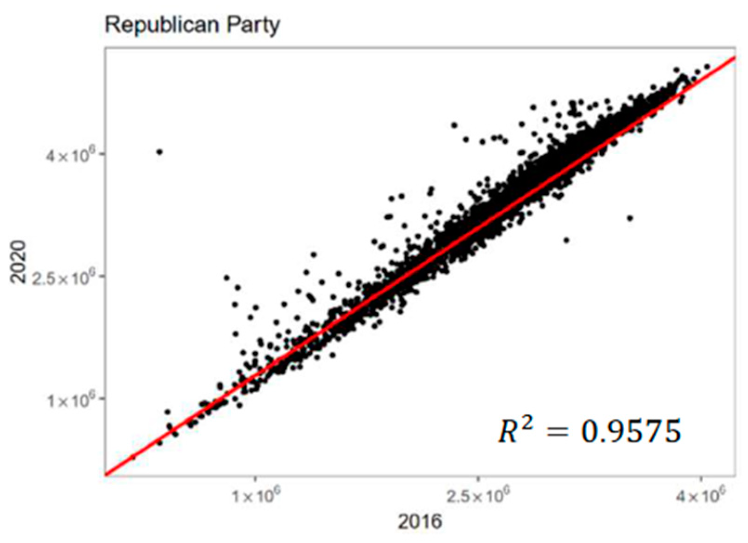
As we discussed in our opening remarks, a linear relationship has also been observed between the estimates of the election results in the span of a quadrennium. Before proceeding to the definition of the linear regression estimator, in Figure 1 and Figure 2 we present the scatter plots of the variable $t_i/{\pi }_i, 1\le i\le M,$ given that $m=30$ for two consecutive presidential elections.

Remark 2.1.

The value of the determination coefficient $R^2$ is 0.9541 and 0.9575 for the Democratic and Republican candidates, respectively; therefore, the utilization of the next linear model (Definition 2.4) is expected to contribute to the precision of our estimates. The heteroscedasticity observed in the residuals in the previous graphs is addressed with the designation of a new slope ${\beta }_0$ for the fitted line, which is derived from using the weighted least squares method (see Remark 2.2).

In Definitions 2.4 and 2.5, we define the linear regression estimator for clusters of unequal sizes, while linear regression estimators in conjunction with simple random sampling have been used in [16].

Definition 2.4.

The linear regression estimator for cluster sampling designs with probabilities proportional to cluster size is defined as

$$X_{REG}\left(s\right)=X_{HT}\left(s\right)+{\widehat{\beta }}_0\left(s\right)·\left(\mathrm{Y}-Y_{HT}\left(s\right)\right),\hspace{1em}s\in S^m.$$

(16)

We symbolize the sampling space for samples of size m as $S^m$, where each of its elements is represented as $s=\left(x_1,{ x}_2,{ x}_3, \dots , x_m\right)\in S^m.$ Moreover, we have

$${\widehat{\beta }}_0\left(s\right)=\sum _{\mathrm{i}=1}^{\mathrm{m}}\left(\frac{{\mathrm{x}}_{\mathrm{i}}}{{\mathsf{\pi }}_{\mathrm{i}}}-\frac{\widehat{X}}{\mathrm{m}}\right)\left(\frac{{\mathrm{y}}_{\mathrm{i}}}{{\pi }_{\mathrm{i}}^{\prime }}-\frac{\widehat{Y}}{\mathrm{m}}\right)/\sum _{\mathrm{i}=1}^{\mathrm{m}}{\left(\frac{{\mathrm{y}}_{\mathrm{i}}}{{\pi }_{\mathrm{i}}^{\prime }}-\frac{\widehat{Y}}{\mathrm{m}}\right)}^2,$$

(17)

where ${\widehat{X}=X}_{HT}\left(s\right)$ and ${\widehat{Y}=Y}_{HT}\left(s\right), s\in S^m$. In addition, we define the following:

$${\beta }_0=\sum _{\mathrm{i}=1}^M{\pi }_i\left(\frac{{\mathrm{x}}_{\mathrm{i}}}{{\mathsf{\pi }}_{\mathrm{i}}}-\frac{\mathrm{X}}{m}\right)\left(\frac{{\mathrm{y}}_{\mathrm{i}}}{{\mathsf{\pi }}_{\mathrm{i}}^{\prime }}-\frac{\mathrm{Y}}{\mathrm{m}}\right)/\sum _{\mathrm{i}=1}^{\mathrm{M}}{{\pi }_i\left(\frac{{\mathrm{y}}_{\mathrm{i}}}{{\pi }_{\mathrm{i}}^{\prime }}-\frac{\mathrm{Y}}{\mathrm{m}}\right)}^2,$$

(18)

where ${{\pi }_i}_{, }{\pi }_i^{\prime } 1\le i\le M$, are the inclusion probabilities of the clusters in the recent and previous elections, respectively, and ${\beta }_0$ is the regression coefficient that minimizes the suggested variance (23) of the linear regression estimator (16). For the estimation of both the variances of the coefficient ${\widehat{\beta }}_0$, the following equations apply [23]:

$$Var\left(\widehat{\beta }\right)=Var\left({\epsilon }_{i,m}\right)·{\left[\sum _{\mathrm{i}=1}^{\mathrm{m}}{\left(\frac{{\mathrm{y}}_{\mathrm{i}}}{{\pi }_{\mathrm{i}}^{\prime }}-\frac{\widehat{Y}}{\mathrm{m}}\right)}^2\right]}^{-1}$$

(19)

and

$$\widehat{Var}\left(\widehat{\beta }\right)=\frac{{\sum }_{i=1}^m{\left({\widehat{\epsilon }}_{i,m}\right)}^2}{m-2}·{\left[\sum _{\mathrm{i}=1}^{\mathrm{m}}{\left(\frac{{\mathrm{y}}_{\mathrm{i}}}{{\pi }_{\mathrm{i}}^{\prime }}-\frac{\widehat{Y}}{\mathrm{m}}\right)}^2\right]}^{-1},$$

(20)

where

$${\epsilon }_{i,m}=\left(\frac{x_i}{{\pi }_i}-\frac{X}{m}\right)-{\beta }_0\left(\frac{y_i}{{\pi }_i^{\prime }}-\frac{Y}{m}\right), 1\le i\le M$$

(21)

and

$${\widehat{\epsilon }}_{i,m}=\left(\frac{x_i}{{\pi }_i}-\frac{\widehat{X}}{m}\right)-{\widehat{\beta }}_0\left(\frac{y_i}{{\pi }_i^{\prime }}-\frac{\widehat{Y}}{m}\right), 1\le i\le M,$$

(22)

are the residuals of the population and their estimated values.

Remark 2.2.

Coefficients ${\beta }_0$ (2.18) and ${\widehat{\beta }}_0$ (2.17) minimize the Equations (23) and (24), respectively [5]. In addition, during the experimental process, it was observed that the expected value of  ${\widehat{\beta }}_0$, based on n samples, coincided with (2.18). The coefficient ${\beta }_0$ (2.18) is retrieved from the application of weighted least squares method on the population, with the weights being set equal to the inclusion probabilities ${\pi }_i, 1\le i\le M$.

Definition 2.5.

Function (23) is defined as the variance of the linear regression estimator under the premise that ${\pi }_i<1, 1\le i\le M$. We have

$$Var\left(X_{REG}\right)=\frac{m(1-f)}{m-1}\sum _{\mathrm{i}\mathsf{ϵ}\mathrm{A}}{\pi }_{\mathrm{i}}{\left({\epsilon }_{i,m}\right)}^2 ,$$

(23)

where ${\beta }_0$ is the coefficient that minimizes the weighted sum of the squared residuals in Equation (23) and

$$A=\left\{ i, 1\le i\le M | {\pi }_i<1\right\}.$$

For the estimation of (23), we have

$$\widehat{Var}\left(X_{REG}\right)=\frac{1}{m-2}\sum _{\mathrm{i}\in {\mathrm{A}}^{\prime }}{\left({\widehat{\epsilon }}_{i,m}\right)}^2\left[m(1-f)+\frac{{\left(\widehat{Y}-Y\right)}^2}{{\sum }_{\iota =1}^m{\left(\frac{{\mathrm{y}}_{\mathrm{i}}}{{\pi }_{\mathrm{i}}^{\prime }}-\frac{\widehat{Y}}{\mathrm{m}}\right)}^2}\right],$$

(24)

where

$$A^{\prime }=\left\{ i, 1\le i\le m | {\pi }_i<1\right\}.$$

By adjusting the prerequisites of the linear regression theory, the following rule should apply to our datasets [5]:

$$\sum _{i=1}^M{\pi }_i\left[\left(\frac{x_i}{{\pi }_i}-\frac{X}{m}\right)-{\beta }_0\left(\frac{y_i}{{\pi }_i^{\prime }}-\frac{{\sum }_{i=1}^M{y}_i\left({\pi }_i/{\pi }_i^{\prime }\right)}{m}\right)\right]=0.$$

(25)

Furthermore, both the residuals ${\epsilon }_{i,m}$ and ${\widehat{\epsilon }}_{i,m}$ must be uncorrelated, and the variance of the population must be constant. For the validation of the two latter prerequisites, we have used the Breusch–Godfrey (autocorrelation) and Breusch–Pagan (homoscedasticity) tests. Indicatively, we report that for $m=30$ the results of both tests have shown that 95% of the samples provided by the algorithm satisfied the null hypotheses of the aforementioned tests.

Remark 2.3.

For large values of $m (m\ge 30)$, the second term between the brackets of Equations (23) and (24), although negligible, contributes to lowering the number of clusters required to achieve percentage of  $p=95\%$ and, consequently, also increases the accuracy c. The level of bias varies in relation to the variable we are examining (votes of each candidate) and the period in question.

Remark 2.4.

The terms in the sums of (23) and (24) with inclusion probabilities ${\pi }_i=1$ do not contribute to the variance; therefore, they are dismissed. A basic prerequisite for this sampling design to be effective is not to have multiple clusters in the population with that property. Note that ${\pi }_i=m{p}_{i }, 1\le i\le M$.

Definition 2.6.

Let $\widehat{\theta }$ be the estimator of parameter $\theta$. The root of the mean squared error (RMSE) is defined as

$$RMSE\left(\widehat{\theta }\right)=\sqrt{{\rm E}\left[{\left(\theta -\widehat{\theta }\right)}^2\right]}.$$

(26)

3. Preliminary Estimator Comparison

Initially, we opt to compare estimators $X_{\mathrm{C}\mathrm{l},\mathrm{u}}$ and $X_{\mathrm{C}\mathrm{l},r}$ since both are formulated based on simple random sampling. In

Table 1. Estimator comparison ${\mathrm{X}}_{\mathrm{C}\mathrm{l},\mathrm{u}}-{\mathrm{X}}_{\mathrm{C}\mathrm{l},\mathrm{r}}\left(\mathrm{R}\mathrm{a}\mathrm{t}\mathrm{i}\mathrm{o}\right)$.

Partition	Estimator	$\overline{\mathit{p}}$	$\overline{\mathit{c}}$	$\overline{\mathit{R}\mathit{M}\mathit{S}\mathit{E}}$	Clusters (m)	Population Total %
States	$X_{Cl,u}$	-	0.880	3.627 × 107	5	9.87
	Ratio	0.875	0.853	6.109 × 106	5	9.87
	$X_{Cl,u}$	-	0.881	2.978 × 107	7	13.69
	Ratio	0.868	0.842	5.284 × 106	7	13.69
	$X_{Cl,u}$	-	0.884	2.421 × 107	10	19.67
	Ratio	0.864	0.849	4.510 × 106	10	19.67
Counties	$X_{Cl,u}$	-	0.808	3.614 × 107	40	1.28
	Ratio	0.801	0.769	8.547 × 106	40	1.28
	$X_{Cl,u}$	-	0.880	1.913 × 107	150	4.85
	Ratio	0.882	0.865	5.183 × 106	150	4.85
	$X_{Cl,u}$	-	0.910	1.143 × 107	380	12.24
	Ratio	0.909	0.901	3.454 × 106	380	12.24

, we present the values $\overline{p}$ and $\overline{c}$, which are defined as the average of percentages $p$ and $c$ for both candidates. Likewise, with the notation $\overline{RMSE}$, we symbolize the average of their corresponding root of mean squared errors. The quantities mentioned were computed for up to $\mathrm{n}=\mathrm{10,000}$ samples for both partitions.

Remark 3.1.

(a) A major drawback of the variance of the first estimator and its estimation is their sensitivity to the variability of the random variable’s values. Using simple random sampling will make this problem more prominent, resulting in samples that commonly contain clusters with significant differences in their values. This has a negative effect on the accuracy of the predictions, causing great discrepancies in the width of the produced confidence intervals in consecutive independent samplings. On the other hand, selecting samples of elements of similar sizes, despite being helpful in reducing the variance, will not improve the precision of the point estimates, therefore decreasing the accuracy of our predictions.

(b) The magnitude of the Ratio estimator’s variance estimation is strongly benefitted by the existence of a linear relationship between the sizes of each cluster and each candidate’s votes. A similar linear relationship is also present between the total number of valid ballots for each candidate in the span of a quadrennium. Such a relationship will be the focus in Section 4, where we will discuss the viability of the proposed linear regression estimator (2.4).

(c) The two main factors that impact the usability of the Ratio estimator are that firstly is biased, and secondly, if we must calculate a prediction for the total candidate’s ballots, a prior estimation of the total valid ballots (N) is needed.

Based on the previous remarks, we can deduce that the Ratio estimator, even though it is biased, is superior to the linear estimator (2.1) due to the significant difference perceived among their estimated mean squared error levels.

The next comparison will be conducted between the Ratio and Horvitz–Thompson estimators. Following the same procedure as before, we detail the results of this comparison in

Table 2. Estimator comparison, ${\mathrm{X}}_{\mathrm{H}\mathrm{T}}-{\mathrm{X}}_{\mathrm{C}\mathrm{l},\mathrm{r}}\left(\mathrm{R}\mathrm{a}\mathrm{t}\mathrm{i}\mathrm{o}\right)$.

Partition	Estimator	$\overline{\mathit{p}}$	$\overline{\mathit{c}}$	$\overline{\mathit{R}\mathit{M}\mathit{S}\mathit{E}}$	Clusters (m)	Population Total %
States	$X_{HT}$	-	0.952	5.741 × 106	5	20.69
	Ratio	0.875	0.853	6.109 × 106	5	9.87
	$X_{HT}$	-	0.953	4.548 × 106	7	29.07
	Ratio	0.868	0.842	5.284 × 106	7	13.69
	$X_{HT}$	-	0.944	3.424 × 106	10	40.55
	Ratio	0.864	0.849	4.510 × 106	10	19.67
	$X_{HT}$	-	0.942	2.499 × 106	15	55.95
	Ratio	0.874	0.860	3.713 × 106	15	29.41
Counties	$X_{HT}$	-	0.949	6.669 × 106	15	4.65
	Ratio	0.682	0.637	1.166 × 107	15	0.49
	$X_{HT}$	-	0.957	3.908 × 106	40	12.32
	Ratio	0.801	0.769	8.547 × 106	40	1.28
	$X_{HT}$	-	0.959	1.688 × 106	150	35.29
	Ratio	0.882	0.865	5.183 × 106	150	4.85
	$X_{HT}$	-	0.959	6.795 × 107	380	61.40
	Ratio	0.909	0.901	3.454 × 106	380	12.24

.

Remark 3.2.

(a) As mentioned at the beginning of this section, the Ratio estimator is formulated with simple random sampling in mind, whereas the Horvitz–Thompson estimator is typically used in conjunction with sampling designs in which the probabilities are proportional to the sampling unit’s size (pps). If all clusters share the same probability, the latter estimator coincides with the linear estimator of definition 2.1, but its accuracy is vastly improved when the probabilities assigned to the clusters are proportional to their size in the overall population. The application of such a sampling design will result in larger clusters appearing more frequently in our samples.

(b) Taking this statement into consideration, we can deduce that for a set amount of m clusters in the sample, there will be a discrepancy between the amount of population that these samples represent. Based on this remark, to accurately compare the two estimators, we must make sure that the samples used in each method correspond to similar percentages of the population.

(c) The low percentages, p and c, of the Ratio estimator in comparison to the X_HT estimator in both partitions, despite its overall lower mean squared error, lead us to select the latter as the more reliable estimator among the two.

It is evident that selecting the partition of counties provides us with more accurate predictions, i.e., a consistently high value for both percentages and a lower mean squared error, especially for a sufficient number of clusters ($m\ge 40$). As a final note for this comparison, it must be stated that for both estimators, prior knowledge of the total valid ballots in each cluster, or an estimation of it, is mandatory for the calculation of the population total and the inclusion probabilities.

4. Linear Regression Estimator

This section’s goal is to observe the impact of the use of the previously recorded election results on the accuracy of our predictions. To that end, we will be analyzing and evaluating the linear regression estimator that was defined in definitions 2.4 and 2.5 on both the partitions of states and counties. To emphasize the utility of our proposed estimator and its estimated variance, we will be applying it to data sets pertaining to three consecutive presidential elections. Moreover, a linear regression estimator is available in the bibliography [5,6,21].

Ours is constructed using the Horvitz–Thompson estimator, and therefore, it is meant to be used in conjunction with a pps sampling design.

As a first step, in

Table 3. Estimator comparison, ${\mathrm{X}}_{\mathrm{H}\mathrm{T}}-{\mathrm{X}}_{\mathrm{R}\mathrm{E}\mathrm{G}}$.

Partition	Estimator	$\overline{\mathit{p}}$	$\overline{\mathit{c}}$	$\overline{\mathit{R}\mathit{M}\mathit{S}\mathit{E}}$	Clusters (m)	Pop. Total %
States	$X_{HT}$	-	0.952	5.741 × 106	5	20.69
	$X_{REG}$	0.937	0.937	1.433 × 106	5	20.69
	$X_{HT}$	-	0.958	5.045 × 106	6	24.74
	$X_{REG}$	0.953	0.949	1.233 × 106	6	24.74
	$X_{HT}$	-	0.953	4.548 × 106	7	29.07
	$X_{REG}$	0.958	0.952	1.097 × 106	7	29.07
Counties	$X_{HT}$	-	0.949	6.669 × 106	15	4.65
	$X_{REG}$	0.942	0.933	1.461 × 106	15	4.65
	$X_{HT}$	-	0.954	5.079 × 106	25	7.79
	$X_{REG}$	0.950	0.901	1.246 × 106	25	7.79
	$X_{HT}$	-	0.954	4.585 × 106	30	9.43
	$X_{REG}$	0.953	0.875	1.190 × 106	30	9.43
	$X_{HT}$	-	0.951	4.221 × 106	35	10.94
	$X_{REG}$	0.954	0.855	1.162 × 106	35	10.94
	$X_{HT}$	-	0.957	3.908 × 106	40	12.35
	$X_{REG}$	0.961	0.871	1.065 × 106	40	12.35

we will be comparing our proposed estimator to the Horvitz–Thompson estimator on the two partitions that were previously defined for varying sample sizes.

Examining Table 3, we observe that the mean squared error of the regression estimator is significantly lower compared to Horvitz–Thompson’s estimator, while the former still manages to retain a high value for the parameter p. The downside of the increased precision in this case is the lapse of accuracy in the model, mainly because estimator (2.4) is biased. In particular, the accumulation of the point estimates about the estimator’s expected value and the decrease in the width of the associated confidence intervals.

In

Table 4. Estimate comparison, ${\mathrm{X}}_{\mathrm{R}\mathrm{E}\mathrm{G}}$, 2016–2020.

Partition	Estimator	$\overline{\mathit{p}}$	$\overline{\mathit{c}}$	$\overline{\mathit{R}\mathit{M}\mathit{S}\mathit{E}}$	Clusters(m)	Pop. Total %
States	$X_{REG} (2012–2016)$	0.947	0.945	2.261 × 106	5	19.84
	$X_{REG} (2016–2020)$	0.937	0.937	1.433 × 106	5	20.69
	$X_{REG} (2012–2016)$	0.945	0.940	1.779 × 106	6	23.98
	$X_{REG} (2016–2020)$	0.953	0.949	1.233 × 106	6	24.74
	$X_{REG} (2012–2016)$	0.952	0.950	1.601 × 106	7	28.05
	$X_{REG} (2016–2020)$	0.958	0.952	1.097 × 106	7	29.07
Counties	$X_{REG} (2012–2016)$	0.942	0.941	1.699 × 106	15	3.85
	$X_{REG} (2016–2020)$	0.942	0.933	1.461 × 106	15	4.65
	$X_{REG} (2012–2016)$	0.951	0.945	1.329 × 106	25	6.40
	$X_{REG} (2016–2020)$	0.950	0.901	1.246 × 106	25	7.79
	$X_{REG} (2012–2016)$	0.953	0.944	1.208 × 106	30	7.71
	$X_{REG} (2016–2020)$	0.953	0.875	1.190 × 106	30	9.43
	$X_{REG} (2012–2016)$	0.955	0.950	1.053 × 106	40	10.28
	$X_{REG} (2016–2020)$	0.961	0.871	1.065 × 106	40	12.35

, we present the results from the comparison of estimators $X_{REG}$ and $X_{HT}$ in three consecutive presidential elections. We will examine the prerequisites needed to accurately predict the outcome of the popular vote of 2016 using the linear regression estimator in conjunction with the data from 2012. Then, we will repeat the same procedure for the data sets from 2020 and 2016. Through evaluating the following tables, we will gain valuable information about the number of clusters needed for a set mean squared error.

In

Table 5. The 95th percentile for estimated variance.

Candidate	95th Percentile (2020)	${\mathit{m}}^{\prime }$ (2020)	95th Percentile (2016)	${\mathit{m}}^{\prime }$ (2016)
DEM	1.218 × 106	27	1.184 × 106	39
GOP	1.219 × 106	31	1.144 × 106	63
DEM	2.119 × 106	13	2.087 × 106	16
GOP	2.030 × 106	15	1.952 × 106	29

, we define $m^{\prime }$ as the number of clusters needed, such that the estimated variance will be lower than a given bound with a probability of 0.95.

The inclusion of the estimated variance ranges enables us to convey some useful insights about the linear regression estimator’s accuracy. In Table 5, it is evident, regarding the presidential elections of 2020, that in order to achieve an estimated variance of 1.2 × 10⁶ or less, we need about 30 clusters in our sample while achieving the same amount of precision for 2016 would significantly increase the total amount of clusters needed. The average mean squared error between both parties in the elections of 2016 and 2020 for the same number of clusters (30) was also relatively stable at about 1.2× 10⁶, as seen in Table 4. This implies that the level of bias of the linear regression estimator can vary a lot, a fact that can be attributed to the difference in the inclusion probabilities ${\pi }_i$ and ${\pi }_i^{\prime }$. 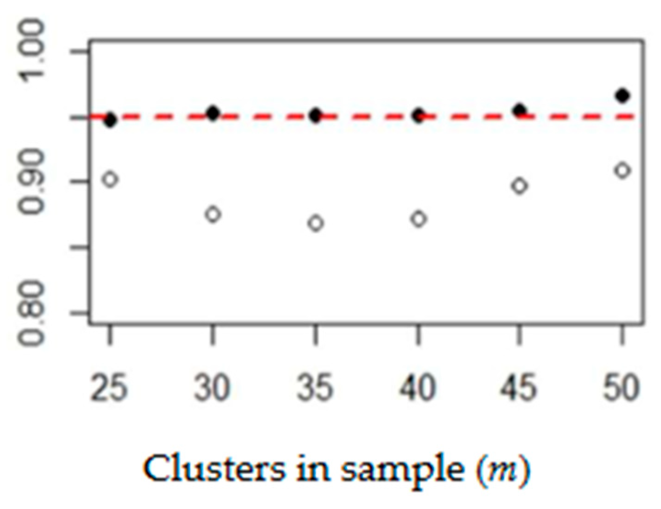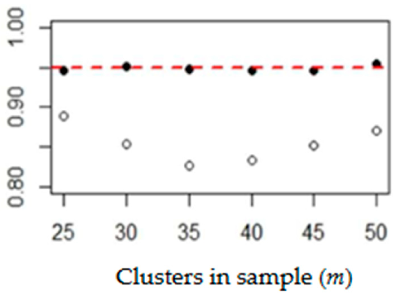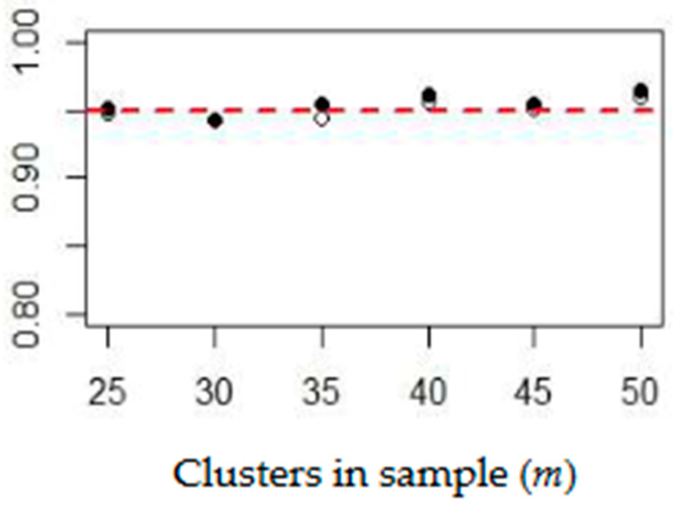In the following graphs, we present the percentages of $p$ and $c$ (black and white dots, respectively) as functions of m for both candidates. The results which correspond to the Democratic Party for the elections in 2020 and 2016 are presented in Figure 3 and Figure 4.

The respective results for the Republican Party are shown in Figure 5 and Figure 6.

As was stated above, the increase in bias observed in the estimations for the quadrennium of 2016–2020 compared to the one preceding it can be attributed to the difference in values of the inclusion probabilities ${\pi }_i$ and ${\pi }_i^{\prime }$. Setting these values as equal in the program diminishes the effects of bias, but it also drastically increases the mean squared error. We emphasize that any major difference between the parameters p and c implies the presence of bias in the model.

In this study, we rely solely on the size of clusters to forecast the outcome of the popular vote. It is highly recommended that the estimates provided by the linear regression model are used as a reference point to be studied in parallel with other prediction models rather than being exclusively relied upon [1]. In particular, the estimations provided by the linear model, due to their innate precision, can be combined with the aforementioned models to increase the efficacy of the prediction of the directional error of a poll.

To conclude this section, in

Table 6. Predictions for the popular vote 2020.

Estimator	$\mathbf{D}\mathbf{E}\mathbf{M}$ $\mathbf{P}\mathbf{e}\mathbf{r}\mathbf{c}\mathbf{e}\mathbf{n}\mathbf{t}$ %	$\mathbf{D}\mathbf{E}\mathbf{M}$ $\mathbf{D}\mathbf{e}\mathbf{v}\mathbf{i}\mathbf{a}\mathbf{t}\mathbf{i}\mathbf{o}\mathbf{n}$ %	$\mathbf{G}\mathbf{O}\mathbf{P}$ $\mathbf{P}\mathbf{e}\mathbf{r}\mathbf{c}\mathbf{e}\mathbf{n}\mathbf{t}$ %	$\mathbf{G}\mathbf{O}\mathbf{P}$ $\mathbf{D}\mathbf{e}\mathbf{v}\mathbf{i}\mathbf{a}\mathbf{t}\mathbf{i}\mathbf{o}\mathbf{n}$ %	Population %—Clusters
$X_{REG}$	51.05	0.73	46.62	0.63	0.9%–15
$X_{H{\rm T}}$	51.73	2.44	46.36	2.48	3.83%–25
$X_{Cl,r}$	52.28	2.31	45.91	2.28	6.47%–250
Results 2020	$DEM$	51.32	$GOP$	46.83

and

Table 7. Predictions for the popular vote 2016.

Estimator	$\mathbf{D}\mathbf{E}\mathbf{M}$ $\mathbf{P}\mathbf{e}\mathbf{r}\mathbf{c}\mathbf{e}\mathbf{n}\mathbf{t}$ %	$\mathbf{D}\mathbf{E}\mathbf{M}$ $\mathbf{D}\mathbf{e}\mathbf{v}\mathbf{i}\mathbf{a}\mathbf{t}\mathbf{i}\mathbf{o}\mathbf{n}$ %	$\mathbf{G}\mathbf{O}\mathbf{P}$ $\mathbf{P}\mathbf{e}\mathbf{r}\mathbf{c}\mathbf{e}\mathbf{n}\mathbf{t}$ %	$\mathbf{G}\mathbf{O}\mathbf{P}$ $\mathbf{D}\mathbf{e}\mathbf{v}\mathbf{i}\mathbf{a}\mathbf{t}\mathbf{i}\mathbf{o}\mathbf{n}$ %	Population %—Clusters
$X_{REG}$	48.03	0.97	47.14	1.09	3.51%–15
$X_{H{\rm T}}$	48.06	2.73	46.83	2.85	4.27%–25
$X_{Cl,r}$	48.89	2.68	46.54	2.65	5.78%–250
Results 2016	$DEM$	47.83	$GOP$	47.30

, we present the point estimates and estimated standard deviation of estimators (2.2), (2.3), and (2.4), along with the results of the popular vote regarding the presidential elections of 2016 and 2020. The samples for each estimator were selected in order to stand for the minimum amount of population needed.

5. Conclusions and Remarks

Considering the data provided in Section 3 and Section 4, we conclude that using the linear regression estimator in the prediction of the popular vote significantly reduces the level of the mean squared error while also maintaining high precision and a sufficient level of accuracy in comparison to the other estimators presented in Section 2 for all sample sizes that were tested. In addition to the goal of accurately predicting the outcome of the election, we can evaluate the efficiency and performance of each estimator on a population scale. In the case of the linear regression estimator, it is imperative that a linear relationship exists between the independent and the response variable in addition to the factors that were described in Section 2, i.e., the constant variance of the residuals and the absence of autocorrelation among them. The disadvantages of the estimator (2.4) can be summarized in two points. Primarily, the linear regression estimator is known to be biased, and as we observed that the level of bias is not consistent even in consecutive elections [5]. Even though this hinders the accuracy of the predictions, it is not as detrimental, as we can deduce by inspecting Table 4. Secondly, to use estimator (2.4), an estimation of the clusters’ size is needed, which can be acquired by knowing the total valid ballots in each cluster at the time of the prediction.

During the conduct of comparisons in Section 3 and Section 4 it was ascertained that utilizing the partition of the counties leads to more accurate predictions. In the case of estimator (2.4), by inspecting the data provided by Table 5, we can discern that 95% of the total estimations of its variance will not exceed 1.2 million when $m^{\prime }$ belongs in the interval [27, 39] for the prediction of the total votes of the Democratic Party and in the interval [31, 63] for the Republican Party. It is possible to infer the outcome of the election using smaller samples, as evident in Table 6 and Table 7, but doing so will increase the mean squared error. Specifically, for $m^{\prime }\in [13, 16]$ and $m^{\prime }\in [15, 29]$ of the former and latter parties, respectively, the estimated variance will not exceed 2.1 million in 95% of the samples. Furthermore, if we require the mean squared error to not surpass 1.2 million, we will need a sample consisting of at least 30 clusters regardless of the period we are discussing (2016 or 2020). The high range of the values contained in the intervals above ensures that any predictions made using the model suggested will not have their accuracy severely impacted by popular vote inversions such as the one observed in the presidential election of 2016. The restrictions we set for the estimated variance correspond to a coefficient of variation (cv) less than or equal to 0.01 and 0.025 for the elections of 2020 and 2016. The slight lapse in accuracy that is noticed in the election of 2020 of the estimator (2.4) can be easily counteracted by setting the confidence level to 99% without incurring a major increase in the width of the produced confidence intervals. Finally, we recommend the partition of the counties as the default partition due to the lower mean squared error, the higher accuracy (c) of the estimations that are derived from it, and the lower required percentage of the population.