1. Introduction
The World Health Organization (WHO) defines a pandemic as an epidemic that occurs worldwide, or over a very large area, affecting many people across different countries [
1]. Throughout history, humanity has been confronted with numerous pandemics. The so-called “Black Death” afflicted Europe from 1348 to 1351, resulting in the mortality of approximately one-third of the continent’s population [
2]. In the 19th century, tuberculosis, an infection caused by the bacterium
Mycobacterium tuberculosis (MTB), accounted for nearly 25% of all deaths [
3]. Another significant example was the Spanish Flu pandemic, also known as the 1918 Flu, which caused the deaths of approximately 100 million people and infected 3% to 5% of the world population [
4,
5].
In January 2020, the world was caught off guard by a novel and highly transmissible disease, subsequently named COVID-19, attributable to the SARS-CoV-2 virus. This epidemic originated in China, specifically in the city of Wuhan, toward the end of 2019, and swiftly disseminated to other nations, formally attaining pandemic status within a few months [
6].
Scientists have determined that the novel virus has a zoonotic origin in bats, which is recognized as a significant viral reservoir. The genetic sequence of SARS-CoV-2 exhibits a 96% similarity to the genetic sequences of other coronaviruses found in bats in China [
7]. Notably, this virus exhibits higher lethality and transmissibility compared to other respiratory infections. It can be transmitted through airborne particles, such as respiratory secretions (cough and saliva), close contact with infected individuals, and the contamination of personal items [
8]. Furthermore, it possesses the capability to persist on surfaces for extended periods [
9].
In Brazil, the first case of the new coronavirus was officially reported by the Ministry of Health on 26 February 2020, in the state of São Paulo. The patient was a 61-year-old individual with a history of recent travel to Italy [
10]. On 12 March, which was fifteen days after the confirmation of the first case in the country, the first fatality attributed to the disease occurred. The deceased was a 57-year-old woman who had been hospitalized with symptoms of COVID-19 one day prior to her passing [
11]. Since that time, the virus has rapidly disseminated throughout the country, leading to a significant increase in fatal cases.
In response to this situation, governors expressed significant concern with the objective of preventing a substantial portion of the population from becoming infected simultaneously. This concern stemmed from the potential to overwhelm the public health system, which could lead to a potential increase in the mortality rate due to the infection. To mitigate the spread of SARS-CoV-2, various measures were implemented, including stringent social distancing restrictions and, in many countries worldwide, the imposition of strict lockdowns.
Since SARS-CoV-2 was a novel pathogen, there was a lack of knowledge regarding its behavior, causing fear and concern among citizens worldwide when the pandemic was declared. Consequently, there was an urgent need to employ tools capable of describing the trajectory of the epidemic, assessing the impact of restrictive measures, forecasting potential virus spread scenarios, and ultimately assisting governments in formulating effective policies to combat COVID-19.
In this context, numerous studies utilizing epidemiological models have been undertaken to comprehend and depict the spread of the virus. These studies involve the estimation of critical epidemiological parameters, including disease transmission rates and the basic reproductive number. For instance, in the study conducted by Ospina et al. (2022) [
12], data-driven analytical tools were employed to discern shifts in the trends of COVID-19 cases and calculate the effective reproductive numbers. Furthermore, several other research efforts have primarily focused on growth models. These models center on the examination of the accumulation of infected cases over a defined time frame and seek to estimate the associated growth rates.
When investigating epidemics, it is important to make predictions to better assist authorities in decision-making, but these predictions are subject to errors. For example, in [
13], the authors examine the accuracy of autoregressive integrated moving average (ARIMA) models, emphasizing their potential for short-term forecasting, even though they are not best suited for long-term predictions. Hence, it would be ideal to find a model that controls this uncertainty the best possible way. Ensemble models are pointed out in the literature as an efficient approach in this regard and, according to [
14,
15,
16], these models allow for an easier determination of a curve that best fits the observed data.
In this study, we initially applied the logistic, Gompertz, and Richards growth models to the data. Nevertheless, in pursuit of enhancing forecast accuracy, we employed ensemble models with a bootstrap approach. This method involves the combination of individual models, thereby integrating predictive precision among them, ultimately providing better control over forecast errors.
The novelty of this research lies in several aspects. Firstly, it employs a comprehensive analysis of COVID-19 cumulative deaths in the State of Paraíba, Brazil, during a critical period, offering insights into the pandemic’s dynamics in a specific regional context. Secondly, the study introduces an ensemble modeling approach, which combines multiple growth models to enhance prediction accuracy, providing a novel solution to the challenges of forecasting the pandemic. This ensemble method’s application in epidemiological modeling is innovative and can be adapted to different infectious diseases.
3. Growth Models and Ensemble Algorithm
Nonlinear growth models are employed to estimate growth rates and have broad applications in various fields, including economics, animal nutrition, the study of infectious diseases, among others. Unlike the SIR compartmental model, growth models rely on the cumulative number of infected cases, which encompasses the sum of the infected and recovered compartments of the SIR model. These models are applied to analyze population growth, specifically to investigate the behavior of S-shaped cumulative curves.
The ensemble models of [
44,
45] have excelled due to their robustness in prediction and forecasting processes [
46,
47]. This approach combines the advantages of many models instead of choosing the best model according to some selection criterion [
44]. One of the advantages is the reduction in prediction and forecasting errors [
48]. In [
16], the authors presented an ensemble model based on bootstrapping that aims to improve precision performance by systematically integrating the predictive precision of each model. This methodology is employed to forecast the evolution of a dynamical growth process defined by a system of nonlinear differential equations, producing more accurate solutions.
The analysis of nonlinear models depends on an iterative process to find solutions to equations because, unlike the linear case, it is generally not possible to find them analytically. The iterative process begins with initial parameter values and calculates the residual sum of squares (RSS) based on these values. The parameters are continuously adjusted until the RSS is minimized.
3.1. Gompertz Model
To describe the growth of solid tumors, mathematician Benjamin Gompertz developed an equation in 1938, now known as the Gompertz equation [
49,
50]. Gompertz observed that, in his model, the growth rate is higher in the earlier stages of the process and rapidly transitions to slower growth. This model is widely applied to describe the general growth of cells, including plants, bacteria, and tumors [
51]. The Gompertz equation is expressed as follows:
Here, C represents the cumulative total of cases, K denotes the maximum number of cumulative cases or the final size of the epidemic, and is the intrinsic per capita growth rate of the infected population.
After solving this ordinary differential equation (ODE), one obtains
where
represents the quantity of cumulative cases at time
t. In this model, the growth is typically smaller in the early and later stages of the outbreak [
52].
3.2. Exponential Model
The exponential model, developed by Thomas Robert Malthus in 1798 [
53], assumes that the rate of change of a quantity
C at time
t is directly proportional to
C. The exponential model is described by
where
represents the exponential growth rate,
N is the population size, and
represents the cumulative number of cases at time
t. Equation (
3) provides the solution to this ordinary differential equation.
where
is the initial number of cases.
3.3. Logistic Model
Mathematician Pierre F. Verhulst proposed a model in 1837 that presumed a population could grow until it reaches its maximum limit, at which point it stabilizes. In this model, the population’s effective growth rate varies with time [
54]. This model serves as an alternative to the exponential growth model, where the growth rate remains constant, and there are no constraints on population growth [
55]. The logistic model is described by the following differential equation:
where
,
C, and
K have the same interpretations presented in the Gompertz model. The solution of this ODE is given by Equation (
5) below
3.4. Richards Model
The Richards model [
56] extends the logistic model by introducing a third parameter,
, which quantifies the deviation from the growth curve. Proposed by Richards in 1959, this model was initially developed to describe the growth of fish populations and represents a generalization of the von Bertalanffy model [
57]. The Richards equation is expressed as the following differential equation:
After solving this ODE, we obtain the Richards model, as shown in Equation (
7):
Here,
K represents the final size of the epidemic,
is the growth rate,
is the number of cases at the onset of the epidemic, and
is the shape parameter that governs the curvature of the curve. When
, Equation (
6) reduces to Verhulst’s logistic growth model [
54] given in (
4).
The introduction of the shape parameter in this model provides greater flexibility in selecting the curve’s shape. The model assumes that the daily incidence curve exhibits a unique peak of high incidence, which corresponds to the inflection point of the epidemic, marking the transition from increasing to decreasing accumulation rates or vice versa. These inflection points can be determined by observing when the epidemic curve begins to decline [
58]. The inflection point
for this model is a function of
and
K and is given by
This quantity holds significant relevance in epidemiology, as it indicates the beginning or end of a phase, representing the moment of acceleration after deceleration or vice versa [
58].
3.5. Performance Metrics
The performance of a particular model can be evaluated using various metrics, including the adjusted coefficient of determination , the mean square error (MSE), and the absolute square error (ASE). These performance criteria all share the common characteristic of considering the model’s residuals, which indicate how closely the fitted results align with the data.
The determination coefficient
, also known as the square of Pearson’s correlation coefficient, is a widely used performance metric in the literature for assessing the quality of a model’s fit to the data. This coefficient ranges from 0 to 1, and the closer it is to 1, the better the fit. This implies that the model can effectively explain most of the response variables [
59,
60]. The calculation of
requires the residual sum of squares (RSS) and the total sum of squares (TSS) as inputs, which are defined as
and
respectively. Here,
n is the number of observations,
represents the
i-th observed value,
is the
i-th fitted value, and
is the mean of all the observations. The adjusted coefficient of determination is then calculated as
The mean absolute error (MAE) is calculated as the average of the absolute differences between the actual parameters and their estimated values. Similarly, the mean square error (MSE) is determined as the average of the squared differences between these values, as expressed in Equations (
8) and (
9), respectively.
The IFMS (interval forecast mean score) assesses the width of the forecast interval by taking into account forecast uncertainty. This is different from metrics such as MAE, MSE, and
, which primarily focus on the discrepancies between the model and the data [
61]. The IFMS is calculated as follows:
where
and
are, respectively, the lower and upper bounds of the forecast interval at time
t at
confidence and
is an indicator function.
3.6. Ensemble Method
The ensemble approach combines the strengths of multiple models through a weighted average, essentially creating a linear combination of nonlinear models. Numerous methods for constructing ensemble models exist in the literature, including neural networks, Bayesian averaging, among others [
62]. However, the method described here is based on the weighted combination of individual models, as proposed in [
16].
Indeed, we can consider a set of
I parametric models, such as
where
represents the parameters that describe the
i-th model. Using the training dataset, the parameter set, and the average ensemble incidence curve for each model
i, estimated for
we calculate the weight
of each model based on the quality of its fit. The quality is assessed using metrics like the mean square error (MSE) or other criteria such as the AIC. In this work, we use MSE to evaluate the quality of the fit. Therefore, the weight for each model is computed as follows:
where
with the constraint that
, ensuring a convex linear combination of models. If
represents the fitted curve by the
i-th model, the
average incidence curve of the ensemble model is given by
In the context of this work, it can be assumed that the observed data (cases) follow a probabilistic structure, which adheres to a Poisson distribution [
16] with a mean of
To obtain a 95% confidence interval (or forecast interval) for the incidence curve at time
t, the parametric bootstrap method can be employed. To do this, consider that the training sample consists of
n data points:
A bootstrap sample is created by generating a random variable
from the Poisson distribution with a mean of
for each data point
, where
:
Therefore, forms a bootstrap sample. This sample is then used to refit each of the I models, calculate weights for each refitted model, estimate parameters, and generate forecasts for the ensemble model. By repeating this process B times, it becomes possible to construct a 95% confidence interval (or forecast interval) based on the 2.5th and 97.5th percentiles.
As an example, consider four individual models given in (
10) from which we will build the ensemble model. Assume
, which corresponds to 100 time points. Here is the step-by-step process:
Fit each of the four models to the original series and estimate the parameters;
Calculate the MSE of each model and find the corresponding weight based on the MSE;
Find the ensemble average incidence curve
Assume that the data follow a Poisson distribution with mean to build a 95% confidence interval (or forecast interval) for the incidence curve at time t using the parametric bootstrap method;
Generate a random variable
for the incidence at each point
,
via the Poisson distribution with mean
, i.e.,
Repeat the process described in the previous step B times to generate B bootstrap replicas and construct the confidence interval;
Refit the I growth models for each replica, calculate the respective MSEs and weights of the refit models, and construct the prediction and forecast intervals for each one;
Obtain B ensemble mean incidence curves using the process described in the previous item, calculate the MSE, and build confidence intervals for each of these mean curves.
4. Results
The exponential, Gompertz, logistic, and Richards models were fitted to the COVID-19 data from the State of Paraíba, Brazil, to study the disease’s growth rates in the State. Subsequently, an ensemble model was constructed using the results from these individual models to produce forecasts ranging from 15 to 30 days ahead. Confidence intervals were also established for each forecasting approach.
The first confirmed COVID-19 case in the State of Paraíba was reported on 18 March 2020. This case involved a 60-year-old man from João Pessoa, who had returned from a trip to Europe on 29 February. Following this initial case, the virus began to spread throughout the State. In response, the Government of Paraíba declared a state of emergency to prevent and combat the pandemic.
Given that the under-reporting of deaths due to COVID-19 is typically less severe than the under-reporting of cases (as case reporting often depends on testing availability), this study utilizes the cumulative death curve attributed to the disease in the State of Paraíba. The first COVID-19-related death in Paraíba was recorded on 31 March 2020, exactly 14 days after the first confirmed case in the State. The deceased individual was a 36-year-old man with diabetes residing in the city of Patos, located in the Sertão region of the State. This man exhibited initial symptoms on 25 March, just six days prior to his passing.
The scope of the pandemic period analyzed in this study encompasses the year 2020, as 2021 was marked by a second wave of the outbreak.
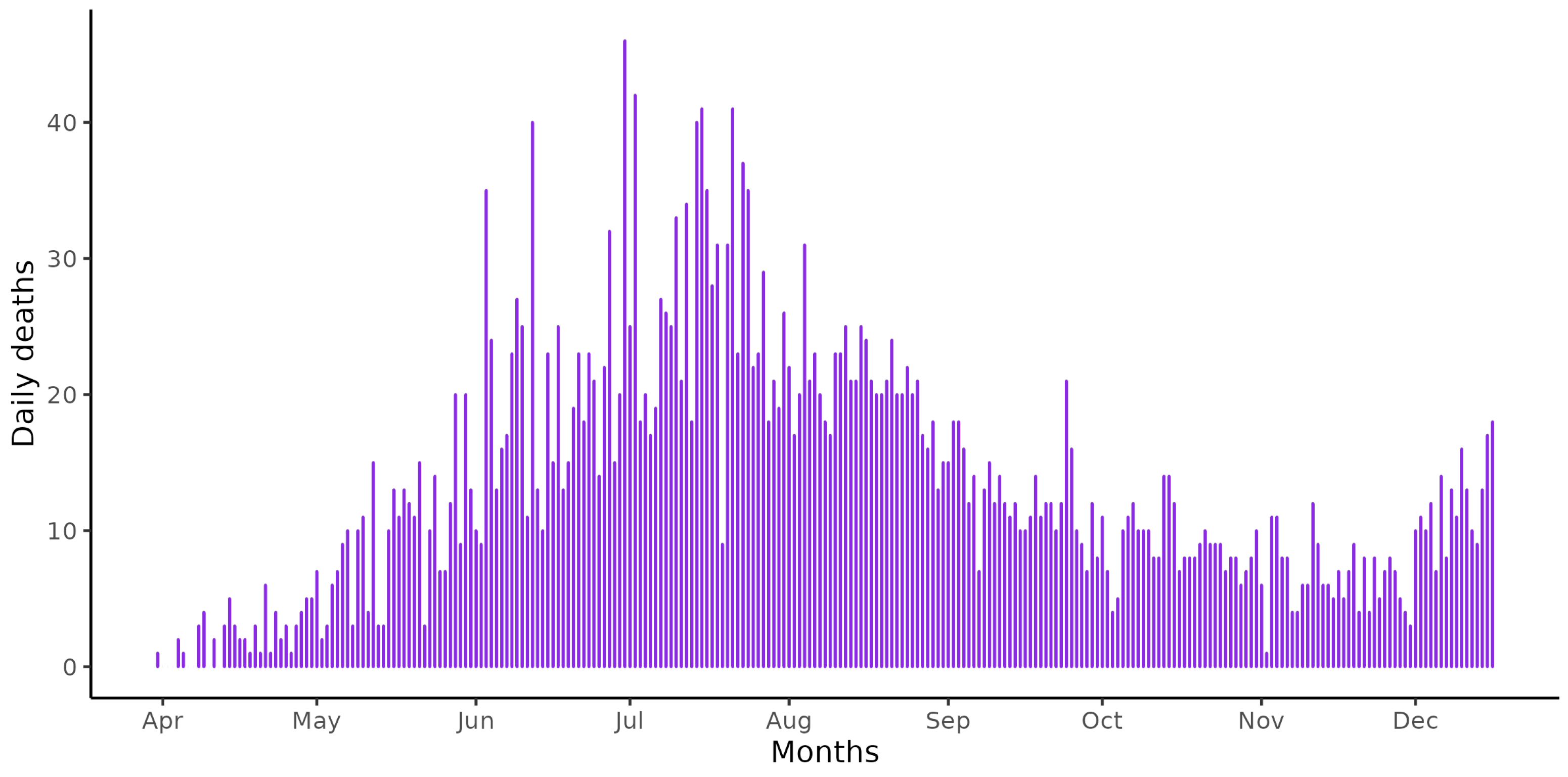
Figure 1 illustrates the daily number of COVID-19 deaths in Paraíba, commencing from the first recorded death until 31 December 2020. Notably, the highest death counts occurred on 25 May and 5 June.
Following this, four growth models were fitted, and an ensemble model was constructed to analyze the death curve in Paraíba and the associated growth rates. The model fitting process considered data spanning from 31 March to 16 December, encompassing a total of 261 days, with the last 15 days of the year reserved for forecasting 15 days ahead. The selected individual models included the exponential, logistic, Gompertz, and Richards growth models.
Figure 2 visually compares the observed cumulative data curve (in orange) with the fitted curve generated by the exponential model (in red). It is evident that the exponential model does not align well with the data, as its curve exhibits a notably different behavior. This discrepancy is likely due to the fact that genuine exponential growth is unattainable in reality, as it would result in unbounded growth, while the total population is inherently limited.
Figure 3 presents the fitted curves generated by the logistic, Gompertz, and Richards models, alongside the cumulative death count reported by the Health Ministry. Additionally, 15-day forecasts were produced for each of these models, with a vertical dashed line indicating the point from which the forecasting starts, relative to 17 December 2020. Upon observing the behavior of these curves, it becomes evident that both the Gompertz and Richards models offer a better fit to the data compared to the logistic model. However, when it comes to forecasting, all three models consistently underestimate the observed death curve. These plots highlight a significant change in the death curve’s behavior just prior to 17 December, making accurate forecasting challenging.
From the fitted growth models, the ensemble model was constructed using the logistic, Gompertz, and Richards models (excluding the exponential model due to its drastically different behavior compared to the data). To create the ensemble model, we calculated the weighted average curve for the growth models based on the mean square error. Next, we generated one thousand (1000) bootstrap replicates using the ensemble model, assuming a Poisson distribution as the counts structure for the weighted average. For each of these replicates, we performed the following steps:
Reconstructed the 95% confidence intervals.
Refitted the logistic, Gompertz, and Richards models.
Built an ensemble model for each replica.
Calculated a new ensemble average curve using the models refitted to the replicas.
Thiscomprehensive process allowed us to generate a robust ensemble model and assess its performance under various conditions and uncertainties.
Table 1 provides the estimated parameters for each growth model and the ensemble model. These parameters include the final size of the pandemic (
K), the growth rate (
), the shape parameter (
), and the corresponding standard errors. Additionally, the table displays the weights assigned to each model based on the mean square error, as explained in
Section 3. The Gompertz model carries the highest weight in the ensemble model due to its lower mean square error (MSQ) compared to the logistic and Richards models. However, the logistic model receives a relatively small weight. Regarding the growth rates, the logistic model estimates a 3.99% growth rate, while the Gompertz model estimates a 1.73% growth rate. In contrast, the Richards model estimates a high growth rate of 8%. The ensemble model’s estimated growth rate falls in between, at 3.54%.
For comparative purposes, we also generated 1000 replicas of the Gompertz, logistic, and Richards models to build the respective confidence intervals and calculate the interval forecast mean score (IFMS).
Table 2 presents forecast performance metrics for each model: the determination coefficient
, the mean absolute error (MAE), the mean square error (MSE), and the IFMS with a 95% confidence level for the cumulative number of deaths. The results indicate that the logistic model had a smaller determination coefficient, with larger MAE and MSE compared to the other models, consistent with the observations in
Figure 3 and the weights assigned to this model (
Table 1). The Gompertz, Richards, and ensemble models showed high determination coefficients (above 0.99), indicating a good fit to the data. Notably, the Gompertz model had the smallest MAE and MSE, outperforming even the ensemble model. Additionally, the confidence intervals constructed using the Gompertz and ensemble models exhibited the smallest IFMS, indicating superior performance in these intervals.
Table 3 displays forecast performance metrics and IFMS for each model. The results indicate that the logistic and Richards models exhibited better fitting performance as measured by MAE and MSE. Additionally, these models had the smallest IFMS, indicating superior interval estimation performance. In
Figure 4, you can see a comparison between the curve fitted by the ensemble model using the original data and the average ensemble curve for the 1000 replicas. It is evident that the ensemble curve and the average ensemble curve for the replicas are very close and fit the data well. However, there is a noticeable deviation in the predictions after the month of October and in the forecast. This difficulty in forecasting deaths may be attributed to the sudden change in the curve toward the end of 2020.
Figure 5 provides a visual representation of the 95% confidence interval constructed for the cumulative number of deaths using the ensemble model. The vertical line marks the starting point of the forecast. It is evident that the interval has a small width, indicating good precision in the interval estimation. While there are a few data points outside the interval boundaries, the distance between these points and the interval is not substantial. Overall, the interval appears to satisfactorily capture the observed death curve.
After generating the ensemble model replicas, the growth models were refitted to each of the 1000 replicas, resulting in 1000 fitted curves for each of the three models. Subsequently, the MSE, MAE, and model weights were recalculated for each replica, and an ensemble curve was constructed for each of them.
Table 4 presents the means of the estimates obtained from these fittings, including the final size of the pandemic
K, growth rate
, shape parameter
, their respective standard errors, and the weights of each model. Notably, the estimates for the final size of the pandemic and the growth rate for the ensemble model were slightly larger than those in
Table 1. This variation is due to changes in the weights assigned to the growth models. The weight for the Gompertz model decreased from 0.6902 (
Table 1) to 0.5649, while the weight of the Richards model increased from 0.2669 to 0.4123. The estimated growth rate was 4.35%, slightly higher than that found for the model with a direct fit to the data.
Table 5 presents the mean performance metrics obtained from the refitted models. These metrics include the determination coefficient
, MAE, and MSE. To calculate the MSE for the ensemble model, each growth model’s weight was multiplied by the respective MSE for the
b-th replica, where
. The average of these MSE values was then computed. The same process was applied to calculate the determination coefficient and MAE. The high MSE value for the logistic model resulted in a significantly lower weight compared to the Gompertz and Richards models. Additionally, it is worth noting that the models refitted to the replicas exhibited a lower average MSE compared to the models fitted directly from the data, including the ensemble model.
Table 6 provides the average values of MAE and MSE for the forecasts produced by fitting the models to the 1000 replicas. The Gompertz model showed the highest MAE and MSE values, contrary to the results observed in the predictions.
It is evident that the forecasts generated by the growth models and the ensemble model did not perform well. Despite the second wave of COVID-19 occurring in 2021, it is noticeable in
Figure 1 that the number of deaths began to increase again around November and December 2020. Consequently, the ensemble model was fitted to the data of registered deaths until 30 September 2020, and forecasts of 15 and 30 days ahead were carried out.
Table 7 provides the results for each growth model, as well as the ensemble model. Among the three growth models, the Richards model had the largest weight in the construction of the ensemble model, which estimated that the growth rate in Paraíba is approximately 8.3%, with a final number of deaths in the state projected to be 3281. (Using the official data, the model estimated that the pandemic would end around 27 November 2020).
Table 8 and
Table 9 display the performance metrics for the predictions and the 15-day ahead forecasts. The determination coefficient suggests that all four models provide a satisfactory fit to the data. The Richards and ensemble models outperformed the others in terms of MAE and MSE for both predictions and 15-day ahead forecasts, which aligns with the higher weight assigned to the Richards model. It is worth noting that the ensemble model exhibited superior forecast performance compared to the individual models.
Figure 6 presents the death curve simulated by the ensemble model and the 15- and 30-day ahead forecasts. The model fits the data perfectly and generates excellent forecasts in both cases. Therefore, it is evident that using data up to the point where the real curve started to accelerate again resulted in better prediction and forecast performance.
Figure 7 displays the confidence interval produced by the ensemble model for the number of registered deaths up to 30 September and the 30-day ahead forecast. The interval performs exceptionally well and closely aligns with the death curve provided by the Ministry of Health.
5. Conclusions
In the early stages of the pandemic, when our understanding of SARS-CoV-2 was limited, numerous scientific studies emerged to address the challenges posed by COVID-19. Among these challenges, the under-reporting of cases has been a significant concern, prompting researchers to explore alternative approaches. To enhance our data analysis, we focused on cumulative death numbers, which offer more stability than daily death counts and are less reliant on the notification of infected cases.
In our study, we employed the logistic, Richards, and Gompertz models to fit COVID-19 death data spanning from March to December 2020. These models were then used to construct an ensemble model. The logistic model exhibited poor performance in fitting the data, while the Richards and Gompertz models displayed better predictive capabilities. However, despite their strong fit to historical data, these models struggled to provide precise forecasts. This challenge became particularly evident in November 2020 when the death curve displayed an unexpected upward trend that the models could not anticipate.
In light of the challenges faced by the individual growth models in accurately forecasting the COVID-19 death data, we turned to the development of an ensemble model. This ensemble approach demonstrated remarkable prediction performance and generated forecasts that closely resembled those produced by the growth models.
It is worth noting that, although the second wave of COVID-19 in Brazil emerged in 2021, there was already an acceleration in the number of deaths during the later months of 2020. As a result, we trained the models using data up to 30 September and conducted forecasts for 15 and 30 days ahead. The ensemble model outperformed the individual growth models in both prediction and forecasting, proving its effectiveness in modeling a single wave of COVID-19 data.


