Article

Efficient Two-Stage Analysis for Complex Trait Association with Arbitrary Depth Sequencing Data

1
Department of Mathematics and Statistics, Wright State University, Dayton, OH 45324, USA
2
Department of Biostatistics, University of North Carolina at Chapel Hill, Chapel Hill, NC 27599, USA
3
Department of Genetics, University of North Carolina at Chapel Hill, Chapel Hill, NC 27599, USA
4
Department of Computer Science, University of North Carolina at Chapel Hill, Chapel Hill, NC 27599, USA
5
Glaxosmithkline, plc, Collegeville, PA 19426, USA
6
Department of Computer Science and Engineering, University of Nebraska-Lincoln, Lincoln, NE 68508, USA
7
Department of Biostatistics and Epidemiology, University of Oklahoma Health Sciences Center, Oklahoma City, OK 73104, USA
8
Merck & Co., Inc., Rahway, NJ 07065, USA
*
Authors to whom correspondence should be addressed.
These authors contributed equally to this work.
Stats 2023, 6(1), 468-481; https://doi.org/10.3390/stats6010029
Submission received: 1 February 2023 / Revised: 14 March 2023 / Accepted: 15 March 2023 / Published: 19 March 2023
(This article belongs to the Section Bioinformatics)

Abstract

:
Sequencing-based genetic association analysis is typically performed by first generating genotype calls from sequence data and then performing association tests on the called genotypes. Standard approaches require accurate genotype calling (GC), which can be achieved either with high sequencing depth (typically available in a small number of individuals) or via computationally intensive multi-sample linkage disequilibrium (LD)-aware methods. We propose a computationally efficient two-stage combination approach for association analysis, in which single-nucleotide polymorphisms (SNPs) are screened in the first stage via a rapid maximum likelihood (ML)-based method on sequence data directly (without first calling genotypes), and then the selected SNPs are evaluated in the second stage by performing association tests on genotypes from multi-sample LD-aware calling. Extensive simulation- and real data-based studies show that the proposed two-stage approaches can save 80% of the computational costs and still obtain more than 90% of the power of the classical method to genotype all markers at various depths  d 2 .

1. Introduction

Next-generation sequencing (NGS) technologies are playing an increasingly important role in genomic studies [1,2]. In recent years, NGS has extended genome-wide association studies (GWAS) from common variants to rare variants in complex trait studies [3,4]. Raw NGS data are short reads from certain genomic regions, which are either aligned to a reference genome or assembled [5,6]. A major challenge with the analysis of NGS data is that it may suffer from multiple types of errors during the process of data generation, such as base-calling and alignment errors, which can cause considerable uncertainty in downstream analysis, especially when sequencing depth is low [5,7]. To quantify this uncertainty, most existing methods for genotype calling from NGS data take a probabilistic framework using the genotype likelihood function (GLF). GLFs incorporate information regarding base calling, alignment, and assembly qualities in addition to simple allele counts and thus take the aforementioned uncertainties into account [5,7].
In the literature, there are mainly two categories of methods to carry out sequencing-based genetic association studies. The methods in the first category first discover polymorphic sites and generate individual-level genotype calls from GLF data at these discovered sites and then perform association testing using the called genotypes [7]. A most crucial step in this category of methods is genotype calling at the detected loci [8,9,10]. When the sequencing depth is high, accurate genotype calling can be achieved when using standard genotype calling for each individual separately [11]. When sequencing depth is low, multi-sample LD-aware methods can be adopted to achieve accurate genotype calling [12,13,14,15]. As individual studies are constrained by their limited budgets, low-depth sequencing with a larger sample size has been established as a more powerful and cost-effective approach than deep sequencing with a smaller sample size [15]. However, multi-sample LD-based algorithms for low-coverage sequencing can be computationally intensive. The computational burden for multi-sample LD-aware genotype calling can, in theory, increase cubically with sample size and will become prohibitive when sample size is in the thousands or tens of thousands [5]. For example, it took one to two weeks to call genome-wide genotypes for 60 CEU individuals sequenced by the 1000 Genomes Pilot Project [5,16]. A novel reference panel-based method, i.e., Genotype Likelihoods IMputation and PhaSing m Ethod (GLIMPSE), has been developed recently to improve efficiency for large-sale studies and reference panels [17]. Rubinacci et al. (2021) showed that GLIMPSE has good performance in low-coverage sequencing data and is extremely efficient in that the computation time mainly depends on the size of reference panel and only grows linearly with the study sample size [17]. A major improvement of GLIMPSE, i.e., GLIMPSE2, has been proposed, with the advantage of computational time scaling sub-linearly with both the number of samples and markers. Rubinacci et al. (2022) used GLIMPSE2 to impute a low-coverage genome from the UKB reference panel with a low computational cost while retaining high accuracy, particularly for rare variants and for very low-coverage samples (0.1×–0.5×) [18].
Methods in the second category, in contrast, perform association testing via a rapid maximum likelihood (ML)-based approach, directly incorporating GLF into the likelihood function for association testing without the intermediate step of calling genotypes [19,20,21,22,23]. The ML-based approach is much faster than the genotype calling-based approach since it avoids multiple-sample LD-aware genotype calling, which is computationally intensive [5].
In this article, we propose a computationally efficient two-stage approach for association analysis on NGS data, which combines advantages of the two categories of methods above. Specifically, candidate SNPs are first screened via a rapid ML-based method, and then only a subset of SNPs with potential associations is evaluated in the second stage by performing association testing on their called genotypes using multi-sample LD-aware methods. In addition, we also apply the proposed two-stage approach to data based on a real NGS dataset [24] from the population-based CoLaus study [25]. Results from simulations demonstrate that our proposed two-stage method can save the considerable burden of genotype calling while still achieving approximately the same power as when genotypes at all SNPs genome-wide are called using multi-sample LD-aware methods. Real data-based analyses show the consistency in reporting significant markers for the two-stage approach with  q < 1  and the full genotyping method ( q = 1 ).
The remainder of this article is organized as follows. We propose our computationally efficient approach for association analysis on NGS data in Section 2, conduct simulation studies to evaluate the performance in Section 3, illustrate the use of our proposed method in real data-based studies in Section 4, provide discussions in Section 5, and draw conclusions in Section 6.

2. Materials and Methods

In this section, we will first briefly introduce existing ML-based tests and genotype calling-based tests for association. We will then present details of our proposed two-stage approach.

2.1. Existing Approaches

Without loss of generality, suppose that a total of n individuals are sequenced on one region of interest. All SNPs are assumed to be bi-allelic. Let  D i  be the observed sequence data for the ith individual,  i = 1 , , n . The goal is to identify SNPs associated with some phenotype of interest by performing single-marker association testing. The phenotype of interest can be binary or quantitative.
In a genotype calling-based approach, individual-level genotypes are first called from the GLF of  D i s via multi-sample linkage disequilibrium (LD)-aware methods [5,7,15,26]. We subsequently perform association testing between each SNP and phenotype of interest based on the called genotypes via standard single-marker tests, for example, classical linear or logistic regression for quantitative or binary phenotypes, adjusting for covariates.
In contrast, in an ML-based approach, the intermediate genotype calling step is skipped. When the phenotype is a case-control status and no covariate adjustment is needed, we can leverage existing methods [19,20,21] to perform likelihood-based tests based directly on the GLF of  D i s. Details to calculate GLF from sequence data and approaches to construct a likelihood function based on GLF can also be found in the literature [19,20,21]. When the phenotype is quantitative or covariate adjustment is needed (which is almost inevitable in real data analysis) for each binary or quantitative phenotype, our previously published UNC-combo method [23] can be used to perform ML-based association testing for either binary or continuous phenotypic outcomes, allowing for covariate adjustment.

2.2. Our Two-Stage Combination Approach

Generally speaking, the performance of ML-based tests is less optimal than those based on genotype calls from multi-sample LD-aware callers, especially when sequencing depth is low. However, on the other hand, the former is computationally much more efficient than the latter as the multi-sample LD aware genotype calling required by the latter is computationally intensive. To combine the advantages of the two different categories of approaches, we propose a computationally efficient two-stage approach for association analysis, in which we employ an ML-based test in stage one to screen candidate SNPs, and then the selected candidate SNPs are evaluated in stage two by performing association tests on SNP genotypes called from LD-aware multi-sample callers.
Specifically, without loss of generality, let m denote the number of SNPs within a genetic region. In stage one, we first perform ML-based single marker tests on each of the m SNPs to obtain m p-values. Afterwards, t ( t = m q 0 < q 1 ) SNPs are selected and carried over into stage two, according to their p-values in ascending order. Theoretically, some LD information would be lost by throwing away non-candidate SNPs with large p-values in stage one, which would in turn potentially impair the accuracy of genotype calling in stage two. However, SNPs in LD with genuine causal SNPs are expected to show some evidence of association with the phenotype of interest. For this reason, we anticipate SNPs in LD with the causal SNP are less likely to be filtered out in the first stage.
Next, we need to specify the number of multiple testing k used to control family-wise type 1 error in the Bonferroni correction in our two-stage testing. Because Stage 1 is only for screening from m markers and Stage 2 conducts tests for  m q ( 0 < q 1 )  markers, the multiple testing k should be less than or equal to m, which is the number of stage one markers. To be conservative, we specify  k = m . We note that both Bonferroni correction and the use of  k = m  is conservative.

3. Simulations

3.1. Simulation Design

We carried out extensive simulations to assess the performance of our proposed two-stage approach. Specifically, we considered two types of designs: (1) a continuous phenotype with covariate adjustment; (2) a binary phenotype with covariate adjustment. We first simulated 45,000 chromosomes (haplotypes) for a 100-kb region using COSI that mimics the LD pattern, local recombination rate, and population history of Europeans using a coalescent model [27]. For quantitative and binary phenotypes with covariate adjustment, we considered two baseline covariates: a binary covariate  X 1  sampled from a Bernoulli distribution with a success probability of 0.5 and a continuous covariate  X 2  sampled from a standard normal distribution.
Quantitative phenotypes were generated via a linear regression model:
Y = α 0 + α 1 X 1 + α 2 X 2 + β G + ϵ
where  α 0 = 1 α 1 = 1 α 2 = 1 ϵ  follows a standard normal distribution; and G denotes the genotype for the causal SNP in this region (for details, see below). Binary phenotypes were generated via a logistic regression model:
logit ( P ( Y = 1 ) ) = α 0 + α 1 X 1 + α 2 X 2 + β G
where  α 0 = 3.65 α 1 = 1 , and  α 2 = 1 . In the design of the binary trait, each simulated sample contained 1000 cases and 1000 controls. In the design of the continuous trait, the quantitative phenotype with covariates, the sample size was 2000. Under the alternative hypothesis, we assumed one causal SNP per simulated dataset and used G to denote its genotype, as in Equations (1) and (2). We considered two scenarios of minor allele frequencies (MAFs) for the causal SNP: 10% and 20%. The effect sizes of the causal SNPs, measured by  β  in Equations (1) and (2), were selected to achieve ∼60% power, according to the sample size and MAF of the causal SNP. We generated 1000 (genotype) datasets for each simulation setting (i.e., design and causal SNP MAF combinations). We generated sequencing data with a per-bp error rate of 0.5% using ShotGun [28]. ShotGun takes a haplotype file as the input. We used COSI-generated haplotypes as the input of ShotGun. ShotGun can generate sequencing data and true genotype data simultaneously. The users need to specify the number of samples, average sequencing depth, other related parameter values, and provide a haplotype file as the input. ShotGun outputs three files: a file containing sequencing data, a file containing true genotypes, and a file containing marker information. The webpage of ShotGun is at https://yunliweb.its.unc.edu//shotgun.html (accessed on 7 Janurary 2023).
For each genotype dataset, we generate four sequencing datasets, with average sequencing depths of 2, 4, 10, and 30, respectively. Furthermore, for each dataset, we used our proposed two-stage approach to select 20%, 40%, and 60% of the SNPs in stage one using a likelihood ratio test [15,23]. In stage two, thunder [15] was used to perform multi-sample LD-aware genotype calling, and SNPs of poor quality (measured by estimated information content) were dropped.

3.2. Simulation Results

3.2.1. Concordance of Estimated Genotypes versus True Genotypes

We first evaluated the concordance between true genotypes and estimated genotypes in the simulation for a range of sequencing depths (d = 2, 4, 10, 30) and a range of screening ratios (q = 0.2, 0.4, 0.6, 1). We report the concordance in the Appendix A in Table A1. The concordance is calculated as the number of matched genotype values divided by the total number of genotype values at genotyped markers. We found that the concordance increases with respect to the sequencing depth (respectively, around 86%, 94%, 99% and 99% concordance for sequencing depths of 2×, 4×, 10× and 30×). Given the same sequencing depth, we found that the concordance is nearly the same for different qs ( q = 0.2 , 0.4 , 0.6 , 1 ).

3.2.2. Consistency between Stage 1 and Stage 2 p-Values

We next evaluated the consistency between Stage 1 and Stage 2 p-values. Table A2 and Table A3 present the average Pearson correlation and average Spearman correlation in our simulation data. We found that both correlations increase with respect to the sequencing depth, d. This means that when the sequencing depth increases, the p-values reported in both tests (Stage 1 and Stage 2) become more consistent. We also found that both correlations decrease with respect to the screen ratio q. This means that when only a proportion of markers is a genotype, the smaller the proportion q, the less consistency between p-values reported by both tests (Stage 1 and Stage 2). In addition, we found that nearly all correlations between Stage 1 and Stage 2 p-values are always positive (99.3% of Pearson correlations and 99.1% of Spearman correlations are positive).

3.2.3. Type 1 Errors without Multiple Test Adjustments

Table 1 and Table 2 present the single-variant type 1 error rate without multiple test adjustment for the binary phenotype and continuous phenotype. We evaluated the performance of our two-stage estimator with screen ratios  q = 0.2 , 0.4 , 0.6 , 1  and the true genotype-based estimator. The true genotype-based estimator is an infeasible estimator, which conducts testing between the phenotype and true genotypes. In comparison, our two-stage estimator selects a proportion (q) of m markers, i.e.,  q m  for genotyping, and then conducts testing between the phenotype and estimated genotypes. Although a true genotype-based estimator is infeasible in practice, we still include it in our performance evaluation to provide some reference values for our simulation. To be more specific, we expect that true genotype-based estimator always have (1) single-variant Type 1 errors without multiple test adjustments controlled, (2) family-wise error rate (Type 1 errors with multiple test adjustment) controlled, and (3) maximal achievable testing power.
Single-variant type 1 errors without multiple-test adjustments were calculated as the average reported significance rate. This is the average rate that a marker is reported to be significant under the null hypothesis that there is no influence on the phenotype from the genotype. A marker is reported to be significant if (1) it is selected in Stage 1, and (2) its Stage 2 p-value <  α , where  α = 0.05  is the significance level. It is the number of reported significant genetic variables divided by total number of genetic variables. This type 1 error, i.e., “average reported significance rate under the null hypothesis”, is expected to be controlled at the significance level,  α , theoretically. In Table 1 and Table 2, we found this type 1 error rate is controlled at a significance level of  α = 0.05  for both our two-stage estimator with screen ratios  q = 0.2 , 0.4 , 0.6 , 1  and our true genotype-based estimator for both the binary phenotype and continuous phenotype.

3.2.4. Type 1 Errors with Multiple Test Adjustment

We next consider the familywise error rate (FWER), i.e., Type 1 errors with multiple test adjustments. We adopted the Bonferroni correction for multiple test adjustments with multiple testing  k = m , where m is the number of genetic markers in Stage 1. A family-wise error occurs under the null hypothesis if any of the m markers are reported to be significant, i.e., its p-value is less than  α / m . For our two-stage testing method, suppose stage two p-values are  P 1 , P 2 , , P q m . A family-wise error occurs if  m i n ( P 1 , P 2 , , P q m ) < α / m , where  α = 0.05 .
Table 3 and Table 4 present the type 1 error rate with multiple test adjustments, i.e., the family-wise error rate (FWER), for the binary phenotype and continuous phenotype for both the two-stage estimator with screen ratios  q = 0.2 , 0.4 , 0.6 , 1  and the infeasible true genotype-based estimator. As can be seen, Type 1 errors in all settings are controlled under 0.05, which justifies our proposed method. We found that some observed FWERs are much smaller than 0.05. This is because both the Bonferroni correction method and the use of multiple testing  k = m  are conservative. We observe that the average number of rare variants ( M A F < 0.05 ) increases with respect to sequencing depth d, whereas the average number of common variants ( M A F 0.05 ) remains nearly the same when sequencing depth increases. We focus on the implementation of our two-stage estimator for common variants in this manuscript. For rare variants, the implementation of our two-stage estimator is stated in the discussion section.
The number of common variants, i.e., m, are different for each simulated dataset, with the average number  = 211.7  and standard deviation  = 69.3 .

3.2.5. Statistical Power Analysis

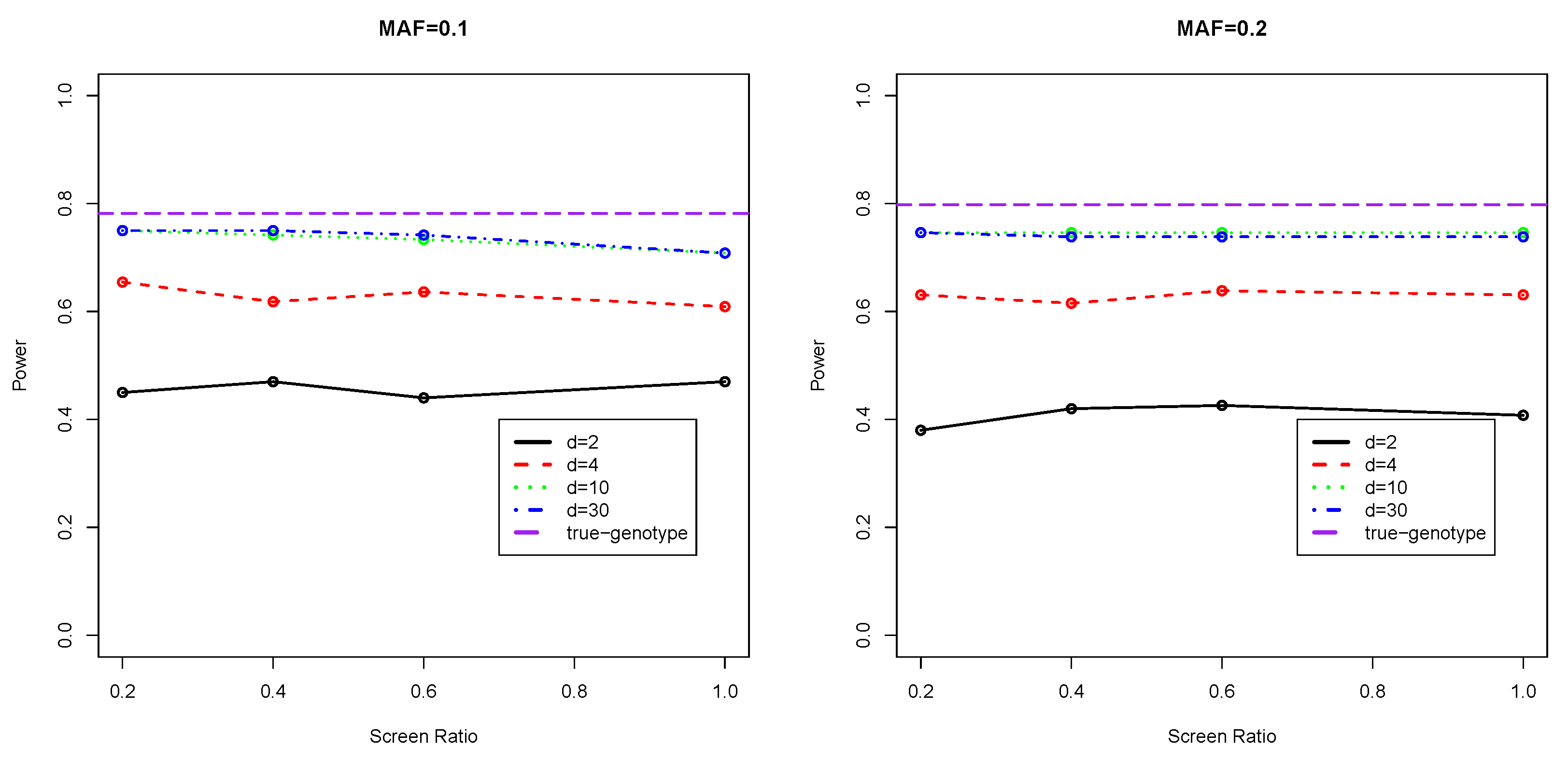
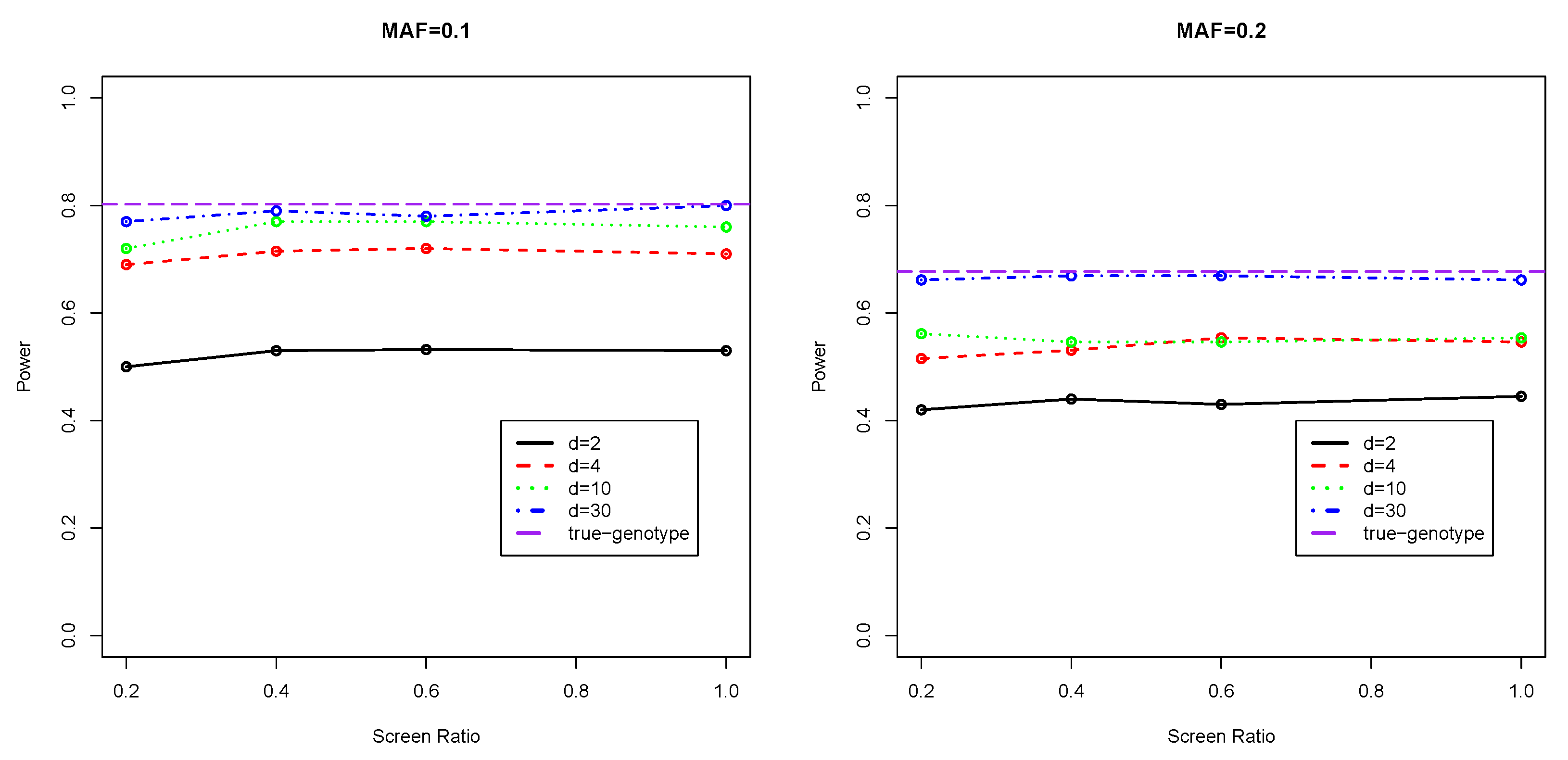
Figure 1 and Figure 2 present the testing powers of our two-stage approach under the various scenarios. We refer to the powers corresponding to screening ratio  q = 1  as full powers as they are obtained when all the genetic regions are genotyped and evaluated via association tests based on genotype calling. As can be seen, the power curves under almost all settings show a fairly flat pattern. With only a proportion ( q = 20 % ) of SNPs of a region selected in stage one and only the selected proportion of markers ( q m  markers) genotyped in Stage two, the use of  q = 20 %  is only around 10% less powerful than the classical method where all SNPs in the region are genotyped ( q = 1 ), which means a considerable saving of computation in genotype calling. Note that the classical method of genotyping all SNPs ( q = 1 ) is still estimated genotype-based, which is less powerful than the infeasible true genotype-based estimator, which, in theory, has the maximal achievable testing power.
THe sequencing depth has a strong effect on the power of association testing. For common variants (MAF ≥ 0.05), the average number of markers remains almost the same when sequencing depth increases from 2× to 30× in our simulated data. We found increasing power when sequencing depth increases.
However, in our previous study, when rare variants were included, this effect did not always go in one direction. Counterintuitively, in some settings, powers of lower-depth sequenced data can be higher than powers of higher-depth sequenced data. This is because sequencing with higher depth not only makes genotype calling more accurate but may also generate more rare-variant SNPs than lower-depth sequencing. The emergence of more rare-variant SNPs means a heavier burden of multiple testing. These two consequences jointly exert opposite effects on the power of multiple association testing, and the final outcome can be in either of the two directions.
We focus on common variants in this paper. For rare variants, the corresponding implementation of our two-stage estimator is proposed in the discussion section. One difference is that rare variants involve group testing, whereas common variants is tested for with a single variant each time, repeating the single-variant testing one by one for common markers.

4. Real Data-Based Studies

We applied our proposed method to a targeted sequencing dataset from the CoLaus study, where 1956 CoLaus subjects from Lausanne (Switzerland) were sequenced at relatively high depth (medium depth 27×) in the exons of 202 genes [24,25]. Seven genes on chromosome X are excluded from the drug-related analysis. A total of 11,496 SNPs were discovered across the 195 autosomal genes among the 1956 subjects. Three SNPs ( G 1 G 2  and  G 3 ) on chromosomes 1, 6 and 11 were chosen to be causal with  p c a u s a l = 0.004 , 0.01 , and 0.15, respectively. The quantitative trait was generated by
Y = α 0 + α 1 X 1 + α 2 X 2 + β 1 G 1 + β 2 G 2 + β 3 G 3 + ϵ ,
where  X 1 X 2  and  ϵ  were generated in the same way as in the simulation study.  α 0 = α 1 = α 2 = 1 β 1 = 1.8 β 2 = 1  and  β 3 = 0.16 . Moreover, the data of two different sequencing depths were simulated by (1) choosing 1 out of every 5 short reads (“Divided by 5”) or (2) choosing 1 out of every 10 short reads (“Divided by 10”). Down-sampling of the sequencing data (1 out of 5 reads, and 1 out of 10 reads) was performed using Samtools software (version: 1.17) (http://www.htslib.org/ (accessed on 7 January 2023)) and AWK linux programming (version 1.3.4).
Similar to the simulation study, 20%, 40%, and 60% of SNPs were screened out in stage one, and the Bonferroni correction was adopted to control Type 1 error.
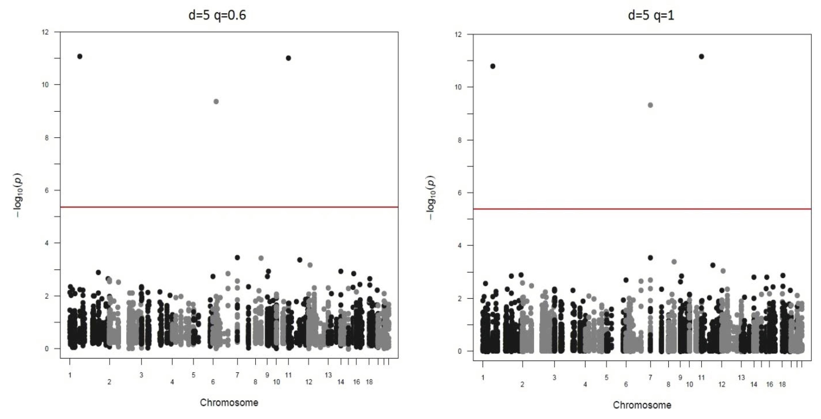
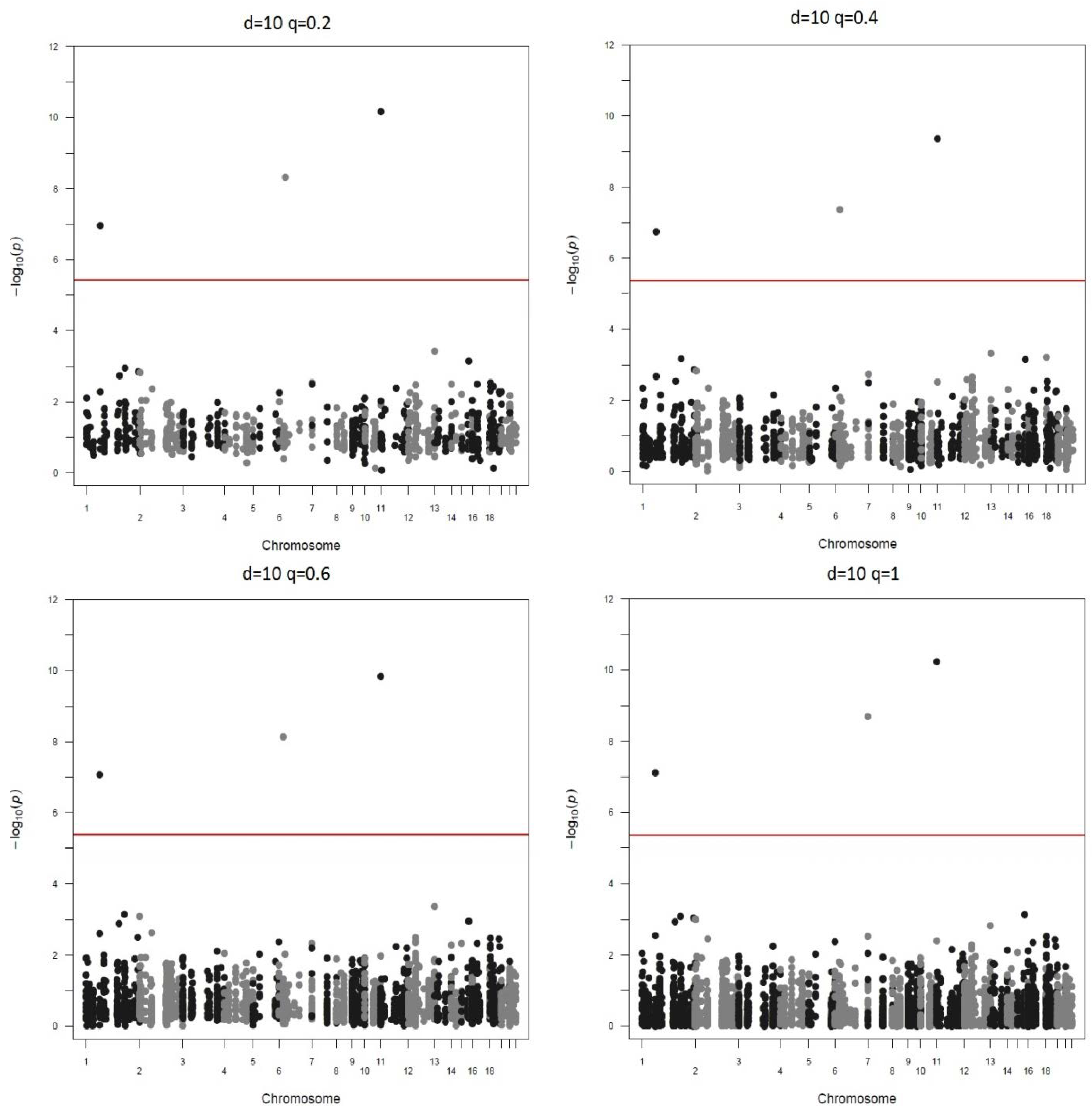
Manhattan plots of the different screen ratios are displayed in Figure 3 and Figure 4. As can be seen, genotyping only 20% SNPs in stage two yields the same three significant markers as the method of genotyping all markers ( q = 1 ).

5. Discussion

We propose a computationally efficient two-stage approach to reduce the burden of the time-consuming LD-aware genotyping process in GWAS studies. In our two-stage approach, raw sequencing data are evaluated via a rapid maximum likelihood-based method directly (without first calling genotypes) in the first stage, and then the selected SNPs are evaluated in the second stage by performing association tests on genotypes from multi-sample LD-aware calling. In the process above, the LD among SNPs associated with the phenotype of interest are well kept after stage one. This approach not only mitigates the computationally intensive genotype calling but also preserves almost all potential associations between SNPs and phenotypes.
In addition to the specific implementation for testing common variants, our two-stage testing method is also proposed as a general framework that allows the selection of sequencing data-based methods in stage one and genotype-based methods in stage two. As a general framework, our two-stage method can work for both common variants and rare variants. For rare variant testing, the genotype-based methods, including burden tests and Sequencing Kernel Association Tests (SKAT), are usually testing for all rare variants within a group [29,30,31]. The group can be gene-based, pathway-based, or range-based. Genome-wide association testing of rare variants will repeat the group testing of one group genome-wide [29,31]. For example, a genome-wide association testing of rare variants can repeat the single-gene rare variant test (for example, the burden test or SKAT test) for all genes genome-wide. Our proposed two-stage testing of rare variants genome-wide is (1) in stage one, conduct sequencing data-based single-gene rare variant tests for all genes genome-wide; (2) in stage two, a proportion of genes (for example 20%) with the smallest p-values in stage one are selected for genotype-based single-gene rare variant testing. Thus, as a general framework, our proposed two-stage method can work for both common variants and rare variants.
However, one issue hindering the implementation of our two-stage method for rare variants is that there are no widely used sequencing data-based rare variant testing methods available in the literature. We are currently working on developing a sequencing data-based rare variant testing method to fill this literature gap. With a suitable sequencing data-based rare variant testing method available, our method can be well-implemented for rare variants. Future work should focus on (1) developing a widely accepted sequencing data-based rare variant testing method without genotype calling, and (2) evaluating the performance of our two-stage testing for rare variants when a widely accepted sequencing data-based rare variant method become available to use as the method in stage one.
The performance of our proposed method depends on the group size of genetic markers due to the use of the Bonferroni correction in our current implementation of two-stage method. The Bonferroni correction is a conservative method in controlling the family-wise error rate (FWER). In addition, we use the number of Stage 1 markers, i.e., m, which is the group size of genetic markers, as the multiple testing k in Bonferroni correction. The use of  k = m  is conservative. Other threshold values can also be used, such as the use of conventional values (threshold =  5 × 10 8  or  10 4 ) and the Benjamini–Hochberg (BH) procedure to control the false-positive rate (FDR) [32]. Future studies will be conducted to evaluate the performance of our methods under various threshold values.
As a general methodology framework, the proposed two-stage approach can be implemented with different association testing methods and software tools used in stage one testing, stage two testing, and genotype calling. Our current implementation is to use the thunder software to implement genotype calling, which is a multi-sample LD-based algorithm. Its computational amount is  O ( q m n 3 ) , where q is the screening ratio, m is the number of markers, and n is the number of samples. Thus, our two-stage testing can save a computational amount of  100 ( 1 q ) % . Future studies will be conducted on the comparison of our current implementation using thunder versus the use of other software, such as the recently developed GLIMPSE and GLIMPSE2 [17,18].
It is critical to control the family-wise Type 1 error in the two-stage approach. The current implementation of our two-stage testing uses the Bonferoni correction with the number of multiple testing (k) equal to the number of genetic markers tested in the first stage, i.e., m. This is because stage one is a preliminary screening procedure for m markers, and stage two is the testing of  q m  markers,  0 < q 1 , so that the total number of multiple testing  k q . Both the Bonferroni correction and the use of multiple testing  k = m  are conservative. To improve statistical performance, other multiple-test adjustment methods, including the Benjamini–Hochberg procedure [32] and the use of refined formulae for multiple testing k, are under our development as an ongoing project. Intuitively, we considered k as a weighted average between the number of genetic variables in stage one, i.e., m, and the number of testing genetic variables in stage two, i.e.,  q m 0 < q < 1 . A more mathematically rigorous derivation of k in the refined formulae is desired in the future work. In our current implementation, we used the Bonferroni correction with multiple testing  k = m . In our study, we evaluated the performance under a range of screening ratios. In practice, we recommend the use of a default screening ratio  q = 20 %  according to our study. Our current study is only on a sequencing depth  d 2 . In our ongoing project, we will evaluate the performance under a scenario with a sequencing depth  d < 2 . A different screening ratio will be proposed for the scenario of sequencing depth  d < 2  as part of our ongoing project.
The proposed two-stage analysis is mainly aimed at improving computational efficiency by reducing the number of genetic markers in genotyping. There are also other types of two-stage analysis in association testing and other bio-statistics areas. For example, the cost-effective two-phase designs consider the scenario that the measurement of some covariate variables is expensive. Inexpensive covariates and outcomes are measured on all subjects in the first phase, and the first-phase information is used to select subjects as measurements of expensive covariates in the second stage. When choosing a sub-sample of subjects, there are statistical methods to minimize the variance of the resulting estimator given budget constraints. Tao et al. (2020) derived the semi-parametric bound of two-stage estimation to improve design efficiency [33]. Yang et al. (2022) formulated it as an optimal problem with precision of selection as the objective function and used the Lagrange multiplier method to solve it [34]. A range of bootstrap methods have been applied to evaluate such precision, including Xu et al. (2020)’s fractional random-weight bootstrap and Brand et al. (2019)’s method combining multiple imputation and bootstrap [35,36]. Future studies will focus on designing and studying the theoretical properties of a two-stage analysis in a more mathematical framework.
6. Conclusions

We propose a computationally efficient two-stage approach to reduce the burden of the time-consuming LD-aware genotyping process in GWAS. We have conducted simulation studies to evaluate the performance, and a real data-based study was carried out to illustrate the use of our method. Our two-stage method has demonstrated the advantage in computational efficiency for sequencing data. In addition, as a general framework, it allows the selection of sequencing data-based methods in stage one and genotype-based methods in stage two.

Author Contributions

Conceptualization, Y.L., Z.X. and S.Y. (Song Yan); methodology, Y.L., Z.X., S.Y. (Song Yan), S.Y. (Shuai Yuan), Z.G., C.W. and S.C.; software, Z.X., S.Y. (Song Yan), Y.L. and C.W.; validation: Y.L., Z.X., S.Y. (Song Yan), S.Y. (Shuai Yuan), C.W. and Z.G.; formal analysis: Z.X., S.Y. (Song Yan), Y.L. and C.W.; investigation: Z.X., S.Y. (Song Yan) and Y.L.; resources: Z.X., S.Y. (Song Yan) and Y.L.; original draft preparation: Z.X., S.Y. (Song Yan), Y.L., C.W. and S.C.; review and editing: Z.X., S.Y. (Song Yan), Y.L., S.Y. (Shuai Yuan), Z.G., C.W. and S.C.; visualization: Z.X., S.Y. (Song Yan), C.W. and Y.L.; supervision: Y.L.; funding acquisition: Y.L.; project administration: Z.X., S.Y. (Song Yan) and Y.L. All authors have read and agreed to the published version of the manuscript.

Funding

The authors wish to acknowledge the NIH support of R01HG006292, R01HG006703, and R01HL129132.

Informed Consent Statement

Not applicable.

Data Availability Statement

All data used in the study are publicly available.

Conflicts of Interest

The author declares no conflict of interest.

Abbreviations

The following abbreviations are used in this manuscript:
COSI Coalescent-Based Simulator
FWER Family-Wise Error Rate
MAF Minor Allele Frequency
GC Genotype Calling
GLF Genotype Likelihood Function
LD Local Disequilibrium
ML Maximum Likelihood
NGS Next Generation Sequencing
SKAT Sequence Kernel Association Test
SNP Single-Nucleotide Polymorphism

Appendix A

Table A1. Concordance between True Genoypes and Called Genotypes in Simulation. Average Sequencing Depth  d = 2 , 4 , 10 , 30 .
Screen Ratio   d = 2   d = 4   d = 10   d = 30
0.20.8570.9410.9930.999
0.40.8630.9420.9930.999
0.60.8630.9420.9930.999
10.8620.9430.9930.998
Table A2. Average Pearson Correlation Between Stage 1 and Stage 2 p-values in Simulation. Average Sequencing Depth  d = 2 , 4 , 10 , 30 .
Screen Ratio   d = 2   d = 4   d = 10   d = 30
0.20.5770.7050.8380.968
0.40.6260.7170.8690.964
0.60.6230.7200.8830.961
10.6120.7250.9060.972
Table A3. Average Spearman Correlation Between Stage 1 and Stage 2 p-values in Simulation. Average Sequencing Depth  d = 2 , 4 , 10 , 30 .
Screen Ratio   d = 2   d = 4   d = 10   d = 30
0.20.5610.6590.7840.928
0.40.6370.7120.8230.938
0.60.6330.7220.8550.950
10.5970.7070.8780.962

References

  1. Levy, S.E.; Myers, R.M. Advancements in next-generation sequencing. Annu. Rev. Genom. Hum. Genet. 2016, 17, 95–115. [Google Scholar] [CrossRef] [PubMed] [Green Version]
  2. Goodwin, S.; McPherson, J.D.; McCombie, W.R. Coming of age: Ten years of next-generation sequencing technologies. Nat. Rev. Genet. 2016, 17, 333–351. [Google Scholar] [CrossRef]
  3. Maher, B. The case of the missing heritability: When scientists opened up the human genome, they expected to find the genetic components of common traits and diseases. But they were nowhere to be seen. Brendan Maher shines a light on six places where the missing loot could be stashed away. Nature 2008, 456, 18–22. [Google Scholar] [PubMed] [Green Version]
  4. Manolio, T.A.; Collins, F.S.; Cox, N.J.; Goldstein, D.B.; Hindorff, L.A.; Hunter, D.J.; McCarthy, M.I.; Ramos, E.M.; Cardon, L.R.; Chakravarti, A.; et al. Finding the missing heritability of complex diseases. Nature 2009, 461, 747–753. [Google Scholar] [CrossRef] [PubMed] [Green Version]
  5. Li, Y.; Chen, W.; Liu, E.Y.; Zhou, Y.H. Single nucleotide polymorphism (SNP) detection and genotype calling from massively parallel sequencing (MPS) data. Stat. Biosci. 2013, 5, 3–25. [Google Scholar] [CrossRef] [Green Version]
  6. Henson, J.; Tischler, G.; Ning, Z. Next-generation sequencing and large genome assemblies. Pharmacogenomics 2012, 13, 901–915. [Google Scholar] [CrossRef] [Green Version]
  7. Nielsen, R.; Paul, J.S.; Albrechtsen, A.; Song, Y.S. Genotype and SNP calling from next-generation sequencing data. Nat. Rev. Genet. 2011, 12, 443–451. [Google Scholar] [CrossRef] [Green Version]
  8. Ley, T.J.; Mardis, E.R.; Ding, L.; Fulton, B.; McLellan, M.D.; Chen, K.; Dooling, D.; Dunford-Shore, B.H.; McGrath, S.; Hickenbotham, M.; et al. DNA sequencing of a cytogenetically normal acute myeloid leukaemia genome. Nature 2008, 456, 66–72. [Google Scholar] [CrossRef] [PubMed] [Green Version]
  9. Bansal, V.; Harismendy, O.; Tewhey, R.; Murray, S.S.; Schork, N.J.; Topol, E.J.; Frazer, K.A. Accurate detection and genotyping of SNPs utilizing population sequencing data. Genome Res. 2010, 20, 537–545. [Google Scholar] [CrossRef] [Green Version]
  10. Li, Y.; Willer, C.J.; Ding, J.; Scheet, P.; Abecasis, G.R. MaCH: Using sequence and genotype data to estimate haplotypes and unobserved genotypes. Genet. Epidemiol. 2010, 34, 816–834. [Google Scholar] [CrossRef] [Green Version]
  11. Bentley, D.R.; Balasubramanian, S.; Swerdlow, H.P.; Smith, G.P.; Milton, J.; Brown, C.G.; Hall, K.P.; Evers, D.J.; Barnes, C.L.; Bignell, H.R.; et al. Accurate whole human genome sequencing using reversible terminator chemistry. Nature 2008, 456, 53–59. [Google Scholar] [CrossRef] [PubMed] [Green Version]
  12. Browning, B.L.; Yu, Z. Simultaneous genotype calling and haplotype phasing improves genotype accuracy and reduces false-positive associations for genome-wide association studies. Am. J. Hum. Genet. 2009, 85, 847–861. [Google Scholar] [CrossRef] [Green Version]
  13. Le, S.Q.; Durbin, R. SNP detection and genotyping from low-coverage sequencing data on multiple diploid samples. Genome Res. 2011, 21, 952–960. [Google Scholar] [CrossRef] [PubMed] [Green Version]
  14. McKenna, A.; Hanna, M.; Banks, E.; Sivachenko, A.; Cibulskis, K.; Kernytsky, A.; Garimella, K.; Altshuler, D.; Gabriel, S.; Daly, M.; et al. The Genome Analysis Toolkit: A MapReduce framework for analyzing next-generation DNA sequencing data. Genome Res. 2010, 20, 1297–1303. [Google Scholar] [CrossRef] [PubMed] [Green Version]
  15. Li, Y.; Sidore, C.; Kang, H.M.; Boehnke, M.; Abecasis, G.R. Low-coverage sequencing: Implications for design of complex trait association studies. Genome Res. 2011, 21, 940–951. [Google Scholar] [CrossRef] [Green Version]
  16. The 1000 Genomes Project Consortium. A map of human genome variation from population-scale sequencing. Nature 2010, 467, 1061. [Google Scholar] [CrossRef] [Green Version]
  17. Rubinacci, S.; Ribeiro, D.M.; Hofmeister, R.J.; Delaneau, O. Efficient phasing and imputation of low-coverage sequencing data using large reference panels. Nat. Genet. 2021, 53, 120–126. [Google Scholar] [CrossRef]
  18. Rubinacci, S.; Hofmeister, R.; Sousa da Mota, B.; Delaneau, O. Imputation of low-coverage sequencing data from 150,119 UK Biobank genomes. bioRxiv 2022. [Google Scholar] [CrossRef]
  19. Kim, S.Y.; Li, Y.; Guo, Y.; Li, R.; Holmkvist, J.; Hansen, T.; Pedersen, O.; Wang, J.; Nielsen, R. Design of association studies with pooled or un-pooled next-generation sequencing data. Genet. Epidemiol. 2010, 34, 479–491. [Google Scholar] [CrossRef] [Green Version]
  20. Kim, S.Y.; Lohmueller, K.E.; Albrechtsen, A.; Li, Y.; Korneliussen, T.; Tian, G.; Grarup, N.; Jiang, T.; Andersen, G.; Witte, D.; et al. Estimation of allele frequency and association mapping using next-generation sequencing data. BMC Bioinform. 2011, 12, 231. [Google Scholar] [CrossRef] [Green Version]
  21. Li, H. A statistical framework for SNP calling, mutation discovery, association mapping and population genetical parameter estimation from sequencing data. Bioinformatics 2011, 27, 2987–2993. [Google Scholar] [CrossRef] [PubMed] [Green Version]
  22. Skotte, L.; Korneliussen, T.S.; Albrechtsen, A. Association testing for next-generation sequencing data using score statistics. Genet. Epidemiol. 2012, 36, 430–437. [Google Scholar] [CrossRef] [PubMed]
  23. Yan, S.; Yuan, S.; Xu, Z.; Zhang, B.; Zhang, B.; Kang, G.; Byrnes, A.; Li, Y. Likelihood-based complex trait association testing for arbitrary depth sequencing data. Bioinformatics 2015, 31, 2955–2962. [Google Scholar] [CrossRef] [Green Version]
  24. Nelson, M.R.; Wegmann, D.; Ehm, M.G.; Kessner, D.; St. Jean, P.; Verzilli, C.; Shen, J.; Tang, Z.; Bacanu, S.A.; Fraser, D.; et al. An abundance of rare functional variants in 202 drug target genes sequenced in 14,002 people. Science 2012, 337, 100–104. [Google Scholar] [CrossRef] [PubMed] [Green Version]
  25. Firmann, M.; Mayor, V.; Vidal, P.M.; Bochud, M.; Pécoud, A.; Hayoz, D.; Paccaud, F.; Preisig, M.; Song, K.S.; Yuan, X.; et al. The CoLaus study: A population-based study to investigate the epidemiology and genetic determinants of cardiovascular risk factors and metabolic syndrome. BMC Cardiovasc. Disord. 2008, 8, 6. [Google Scholar] [CrossRef] [PubMed] [Green Version]
  26. Wang, Y.; Lu, J.; Yu, J.; Gibbs, R.A.; Yu, F. An integrative variant analysis pipeline for accurate genotype/haplotype inference in population NGS data. Genome Res. 2013, 23, 833–842. [Google Scholar] [CrossRef] [Green Version]
  27. Schaffner, S.F.; Foo, C.; Gabriel, S.; Reich, D.; Daly, M.J.; Altshuler, D. Calibrating a coalescent simulation of human genome sequence variation. Genome Res. 2005, 15, 1576–1583. [Google Scholar] [CrossRef] [PubMed] [Green Version]
  28. Kang, J.; Huang, K.C.; Xu, Z.; Wang, Y.; Abecasis, G.R.; Li, Y. AbCD: Arbitrary coverage design for sequencing-based genetic studies. Bioinformatics 2013, 29, 799–801. [Google Scholar] [CrossRef] [Green Version]
  29. Wu, M.C.; Lee, S.; Cai, T.; Li, Y.; Boehnke, M.; Lin, X. Rare-variant association testing for sequencing data with the sequence kernel association test. Am. J. Hum. Genet. 2011, 89, 82–93. [Google Scholar] [CrossRef] [Green Version]
  30. Li, B.; Leal, S.M. Methods for detecting associations with rare variants for common diseases: Application to analysis of sequence data. Am. J. Hum. Genet. 2008, 83, 311–321. [Google Scholar] [CrossRef] [Green Version]
  31. Madsen, B.E.; Browning, S.R. A groupwise association test for rare mutations using a weighted sum statistic. PLoS Genet. 2009, 5, e1000384. [Google Scholar] [CrossRef] [PubMed] [Green Version]
  32. Benjamini, Y.; Hochberg, Y. Controlling the false discovery rate: A practical and powerful approach to multiple testing. J. R. Stat. Soc. Ser. B (Methodol.) 1995, 57, 289–300. [Google Scholar] [CrossRef]
  33. Tao, R.; Zeng, D.; Lin, D.Y. Optimal designs of two-phase studies. J. Am. Stat. Assoc. 2020, 115, 1946–1959. [Google Scholar] [CrossRef] [PubMed]
  34. Yang, C.; Diao, L.; Cook, R.J. Adaptive response-dependent two-phase designs: Some results on robustness and efficiency. Stat. Med. 2022, 41, 4403–4425. [Google Scholar] [CrossRef] [PubMed]
  35. Xu, L.; Gotwalt, C.; Hong, Y.; King, C.B.; Meeker, W.Q. Applications of the fractional-random-weight bootstrap. Am. Stat. 2020, 74, 345–358. [Google Scholar] [CrossRef]
  36. Brand, J.; van Buuren, S.; le Cessie, S.; van den Hout, W. Combining multiple imputation and bootstrap in the analysis of cost-effectiveness trial data. Stat. Med. 2019, 38, 210–220. [Google Scholar] [CrossRef] [Green Version]
Figure 1. Testing Powers of Binary Phenotype with Covariates Adjusted.
Stats 06 00029 g001
Figure 2. Testing Powers of Continuous Phenotype with Covariates Adjusted.
Stats 06 00029 g002
Figure 3. Real data-based studies when down-sample ratio is 5.
Stats 06 00029 g003aStats 06 00029 g003b
Figure 4. Real data-based studies when down-sample ratio is 10.
Stats 06 00029 g004
Table 1. Type 1 Errors without Multiple Test Adjustment for Binary Phenotype with Average Sequencing Depth  d = 2 , 4 , 10 , 30  for Two-Stage Estimator and True Genotype-Based Estimator.
EstimatorScreen Ratio   d = 2   d = 4   d = 10   d = 30
Two-Stage0.20.0450.0490.0410.044
Two-Stage0.40.0480.0530.0460.050
Two-Stage0.60.0470.0490.0470.049
Two-Stage10.0460.0470.0470.049
True-GenoNA 10.052
1 The true genotype-based estimator does not involve the screening step so that there is no screen ratio.
Table 2. Type 1 Errors without Multiple Test Adjustment for Continuous Phenotype with Average Sequencing Depth  d = 2 , 4 , 10 , 30  for Two-Stage Estimator and True Genotype-Based Estimator.
EstimatorScreen Ratio   d = 2   d = 4   d = 10   d = 30
Two-Stage0.20.0480.0430.0420.044
Two-Stage0.40.0520.0500.0500.050
Two-Stage0.60.0520.0510.0510.049
Two-Stage10.0500.0520.0510.050
True-GenoNA 10.051
1 The true genotype-based estimator does not involve the screening step so that there is no screen ratio.
Table 3. Type 1 Errors with Multiple Test Adjustments for Binary Phenotype with Average Sequencing Depth  d = 2 , 4 , 10 , 30  for Two-Stage Estimator and True Genotype-Based Estimator.
EstimatorScreen Ratio   d = 2   d = 4   d = 10   d = 30
Two-Stage0.20.0280.0100.0130.010
Two-Stage0.40.0250.0130.0100.010
Two-Stage0.60.0150.0100.0130.007
Two-Stage10.0200.0130.0100.007
True-GenoNA 10.018
1 The true genotype-based estimator does not involve the screening step so that there is no screen ratio.
Table 4. Type 1 Errors with Multiple Test Adjustments for Continuous Phenotype with Average Sequencing Depth  d = 2 , 4 , 10 , 30  for Two-Stage Estimator and True Genotype-Based Estimator.
EstimatorScreen Ratio   d = 2   d = 4   d = 10   d = 30
Two-Stage0.20.0350.0280.0210.019
Two-Stage0.40.0320.0300.0230.023
Two-Stage0.60.0300.0250.0210.023
Two-Stage10.0340.0330.0230.015
True-GenoNA 10.021
1 The true genotype-based estimator does not involve the screening step so that there is no screen ratio.
Disclaimer/Publisher’s Note: The statements, opinions and data contained in all publications are solely those of the individual author(s) and contributor(s) and not of MDPI and/or the editor(s). MDPI and/or the editor(s) disclaim responsibility for any injury to people or property resulting from any ideas, methods, instructions or products referred to in the content.