Article

The Linear Skew-t Distribution and Its Properties

1
Sheffield University Management School, University of Sheffield, Sheffield S10 1FL, UK
2
UCD Michael Smurfit Graduate Business School, University College Dublin, Carysfort Avenue, Blackrock, D04 V1W8 Dublin, Ireland
Stats 2023, 6(1), 381-410; https://doi.org/10.3390/stats6010024
Submission received: 2 December 2022 / Revised: 15 February 2023 / Accepted: 16 February 2023 / Published: 23 February 2023

Abstract

:
The aim of this expository paper is to present the properties of the linear skew-t distribution, which is a specific example of a symmetry modulated-distribution. The skewing function remains the distribution function of Student’s t, but its argument is simpler than that used for the standard skew-t. The linear skew-t offers different insights, for example, different moments and tail behavior, and can be simpler to use for empirical work. It is shown that the distribution may be expressed as a hidden truncation model. The paper describes an extended version of the distribution that is analogous to the extended skew-t. For certain parameter values, the distribution is bimodal. The paper presents expressions for the moments of the distribution and shows that numerical integration methods are required. A multivariate version of the distribution is described. The bivariate version of the distribution may also be bimodal. The distribution is not closed under marginalization, and stochastic ordering is not satisfied. The properties of the distribution are illustrated with numerous examples of the density functions, table of moments and critical values. The results in this paper suggest that the linear skew-t may be useful for some applications, but that it should be used with care for methodological work.

1. Introduction

The skew-normal distribution was introduced in [1] and the skew-t distribution in [2]. These two distributions share the property that they may be derived formally. There are several methods of derivation of which probably the best known is to consider the bivariate normal distribution of two random variables X and Y, each with zero mean, unit variance and correlation ρ . The skew-normal distribution arises by then considering the distribution of X conditional on Y 0 ( Y 0 ). There is a similar and equally well-known construction for the skew-t. As well as these formal foundations, the construction corresponds to situations in which the X variable is sampled only if the second variable Y takes non-negative (nonpositive) values. Applications where such situations arise are well-known. As Y is not explicitly observed, these models have been referred to as hidden truncation models; see, for example, [3]. As well as the skew-t distribution derived formally in [2], the earlier paper by [4] shows that other more flexible constructions may be employed. Lemma 1 of [4] that paper shows that a skew-elliptical distribution may be constructed using an elliptically symmetric distribution and the distribution function corresponding to a density function that is also symmetric. In its simple form, the resulting skew-elliptical density function takes the form
f x = 2 g x G λ x ,
where g . denotes a density function of a random variable that is symmetrically distributed about zero. The skewing term G . denotes the distribution function of a random variable that is also symmetrically distributed about zero. The distribution at Equation (1) is often referred to as a symmetry-modulated distribution, with λ being called the shape or skewness parameter. There is a substantial development of this work in [5], with further results in [6]. Ref. [7] present a somewhat different construction that may nonetheless be regarded as a symmetry-modulated distribution.
The skew-elliptical distribution considered in this paper is a specific form of Equation (1) and is based on the Student’s t distribution. In the usual notation, the density function of a random variable X is
f x = 2 t ν x T ν + 1 λ x .
In this paper, this distribution is referred to as the linear skew-t, abbreviated to LST. With this construction, a minor extension that may be useful in some cases is
f x = 2 t ν x T ω λ x .
That is, for this distribution, there is no essential reason for there to be a correspondence between the two degrees of freedom parameters ν and ω . However, for reasons that follow from Proposition 1 below, the majority of the technical results in this paper impose the restriction ω = ν + 1 . This distribution may be attractive for applied work because it is simpler in structure than the usual Azzalini skew-t, henceforth ST. In addition, as the paper shows, there are combinations of parameter values under which the shape of the two distributions differs. The use of the LST does not seem to be widespread, with the paper by [8] being an exception. It is straightforward to construct a multivariate version for an n-vector X . Once again, in the usual notation, the density function corresponding to Equation (2) is
f x = 2 t n , ν x T ν + n λ T x .
The aim of this expository paper is as follows. First, it is to investigate whether or not the linear skew-t distribution at Equation (2) and the multivariate version at Equation (4) may be derived as a hidden truncation model or scale mixture and, if so, whether the implied mechanisms are realistic. Secondly, as there are differences between the LST and the ST, the paper presents some properties of the distribution, namely the first four moments and critical values. These are compared with the corresponding values for the ST. Thirdly, the paper investigates and compares extended versions of the two distributions, LEST and EST, respectively. Extended versions are important for some methodological developments and empirical applications because they offer greater flexibility in the shape of the distributions, and hence in moments and critical values. The paper also presents results for multivariate distributions. Finally, reflecting the results reported in Section 3.1 of [5], the paper reports results for stochastic ordering with respect to shape for the LEST and EST distributions.
The paper has the following sections. Section 2 contains a review of the literature that summarizes developments in skew-elliptical and related distribution theory. Section 3 contains results and resulting properties for the ST distribution. Section 4 describes the corresponding results for the extended version. This distribution is similar in construction to the extended skew-t first referred to in [2] and described in more detail in [9,10]. Results for multivariate versions of the distribution are in Section 5. Section 6 is concerned with stochastic ordering with respect to the shape parameter λ of both the LEST and EST distributions. Section 7 contains concluding remarks and a short discussion. There is an appendix containing technical details of some of the results.
This paper contributes to the literature on symmetry-modulated distributions by providing specific results based on Student’s t distribution. The paper describes an extended version of the distribution that is analogous to the extended skew-t. For certain parameter values, the properties of the distribution are different from those of the skew-normal or skew-t. This feature creates the possibility of new application areas in empirical work. It is shown that for certain parameter values, the distribution is bimodal, a feature not exhibited by the skew-normal or skew-t.
The notation t ν x denotes the Student’s density function with ν degrees of freedom, and t ν x ; μ , σ 2 denotes the density function with location μ and scale σ . When not defined explicitly, other notation is that in common use. Density and distribution functions are denoted by f . and F . , respectively. As their use is clear from the context, these notations are used without subscripts. Standardized distributions with μ = 0 and σ = 1 are used throughout. Tables and figures that illustrate algebraic results are based on λ = 1 , 2 , 5 and 10 and a range of values for ν and the extension parameter τ .

2. Literature Review

The seminal work by [1] has led to a large literature whose growth continues and whose scope expands. In toto, there are far too many articles to cite in a single paper, but there is a selective overview in [11]. From the perspective of this paper, which is concerned with the specific form of distribution at Equation (1), ref. [5], A&R2012 henceforth, serves as a benchmark for recent research. Perhaps surprisingly, it has been cited by numerous authors who employ it to support the use of the skew-normal distribution in a range of applications. Ref. [12] used the skew-normal distribution in statistical process control. More recent examples include applications in astronomy and astrophysics [13,14,15,16], seemingly unrelated regression [17] and the weather [18,19].
The results in A&R2012, in particular those in Section 3.1, are developed in [20,21] in two papers about the shape parameter. These results are extended in [22], who introduce the mode invariance in the family of distributions introduced in [21]. Mode invariance facilitates the study of various properties of the distribution. Ref. [23] is concerned with stochastic dominance. Ref. [24] develops a procedure to allow stochastic ordering for the multivariate skew-normal distribution. Stochastic ordering methods for the multivariate normal mean–variance and skew-normal scale–shape mixture models are described in [25]. There are related results in [26]. Ref. [27] presents results for the expected value and characteristic function of the matrix variate skew-normal distribution and applies the results to stochastic ordering. Ref. [28] employs the results in A&R2012 to develop classification procedures across groups for situations in which marginal distributions are skew-symmetric.
As stated in the introduction, this paper is concerned with the properties of a specific form of Equation (1) based on Student’s t. There are many other papers that are concerned with the development of specific probability distributions that exhibit asymmetry. Some show a close connection to the original skew-normal or skew-t ones, although others do not. Ref. [29] presents a multivariate skew-Cauchy distribution. This differs from the conventional multivariate skew-t in that the unobserved variables are independently distributed. The same concept is extended in [30], in which the unobserved variables are constrained. It is notable that some of the exemplar distributions in this paper are bimodal. Ref. [31] presents a number of different univariate distributions based on specific forms of Equation (1). These include, for example, the skew-Laplace distribution. Ref. [32] is a similar paper which presents detailed properties based on several underlying forms of f . and G . . These include the exponential power distribution and a distribution based on the modified Bessel function of the second kind (See Chapter 9 of [33] for further details). The former is due originally to [34], and the latter to [35]. Ref. [36] presents a distribution based on a generalization of Student’s t in which the familiar x 2 term is replaced by | x | k , with corresponding changes to the normalizing constant.
Ref. [37] describes a general approach to the construction of distributions that are bimodal and which are based to some extent on Equation (1). In these constructions, the density function is
f x = α g x G x α 1 ; α R ,
where G . is now an absolutely continuous distribution function and g . is the corresponding density. Ref. [38] introduces distributions that may be referred to collectively as skew-flexible. In their Theorem 2.1, and using the notation of Equation (1), the density function is
f x = c δ g | x | + δ G λ x ; δ , λ R ; c δ = G ¯ δ 1 ,
where G ¯ . is the distribution function corresponding to g . . This distribution is bimodal for certain values of δ . In a very recent paper, ref. [39] extended earlier results due to [40,41]. Specifically, ref. [39] studies the extended half-skew normal distribution with density function h x , given by
h x = c α , λ α + x 2 α + 1 f x ; x 0 , α > 0 , λ R ,
where c α , λ is the normalizing constant and f . is defined at Equation (1) with G . = Φ . . Ref. [42] develops a weighted skew-normal model in which the density is
f x = w x , θ g x G λ x E w X , θ ,
where g . and G . are as defined at Equation (1), w . is a weight function and θ is a parameter which may be vector valued. According to the authors, weighted distributions were introduced by [43] and offer flexible models for analyzing data sets. Ref. [44] describes the properties of a specific form of Equation (8) in which the weight function satisfies
w x , α = 1 + α x 2 2 1 + α ,
and the underlying density function is skew-normal. Depending on their parameterization, skewed distributions can be bimodal. Ref. [45] describes such a distribution and provides a useful list of relevant references. Recently, [46] proposed a multivariate distribution, which they term robust. In their paper, an elliptically symmetric density of a random vector X is multiplied by a skewing function of the form
G m λ T x = Π i = 1 m G λ i T x .
In a different type of development, ref. [47] presents a number of bivariate and multivariate log-normal distributions. These distributions constitute a different family from those summarized above. However, they do exhibit asymmetry and, as the authors argue, may be used for many financial data sets.
To summarize, development of probability distributions based on work by Azzalini and many of his co-authors remains an active area of research, as does the appearance in the literature of asymmetric distributions that have a different genesis.

3. The Linear Skew-t Distribution

This section describes the basic properties of the LST distribution at Equation (2). Proposition 1 shows that the density function arises as a scale mixture. To illustrate similarities and differences, the section also presents comparable results for the standardized form of the skew-t distribution.

3.1. The Underlying Hidden Truncation Model

Proposition 1.
Conditional on X = x and S = s , assume that Y has a normal distribution with expected value λ x 1 + x 2 / ν and variance 1 / s . Furthermore, assume that the conditional distribution of X given S = s is N 0 , 1 / s , with S∼ χ ν 2 / ν . The following result holds: the density function of X given that Y > 0 is
f x = 2 t ν x T ν + 1 ν + 1 / ν λ x .
The proof follows by direct verification, with details in Appendix A.
The density function for the standardized skew-t distribution, abbreviated to SST, is
f x = 2 t ν x T ν + 1 ν + 1 ν + x 2 λ x .
It is clear that for given ν and λ , values of the two density functions are different. However, the limiting cases as ν are the same; that is, the standardized skew-normal.
f x = 2 ϕ x Φ λ x .
As λ , the limiting case distribution at Equation (13) is the truncated or half-normal distribution whose density function is 2 ϕ x ; x 0 . A similar result holds for distributions at Equations (11) and (12). In both cases the limiting distribution is a truncated or half-t with density function 2 t ν x ; x 0 . To avoid unnecessary duplication, this result is presented more formally in Section 4, which is concerned with extended versions of the distributions.
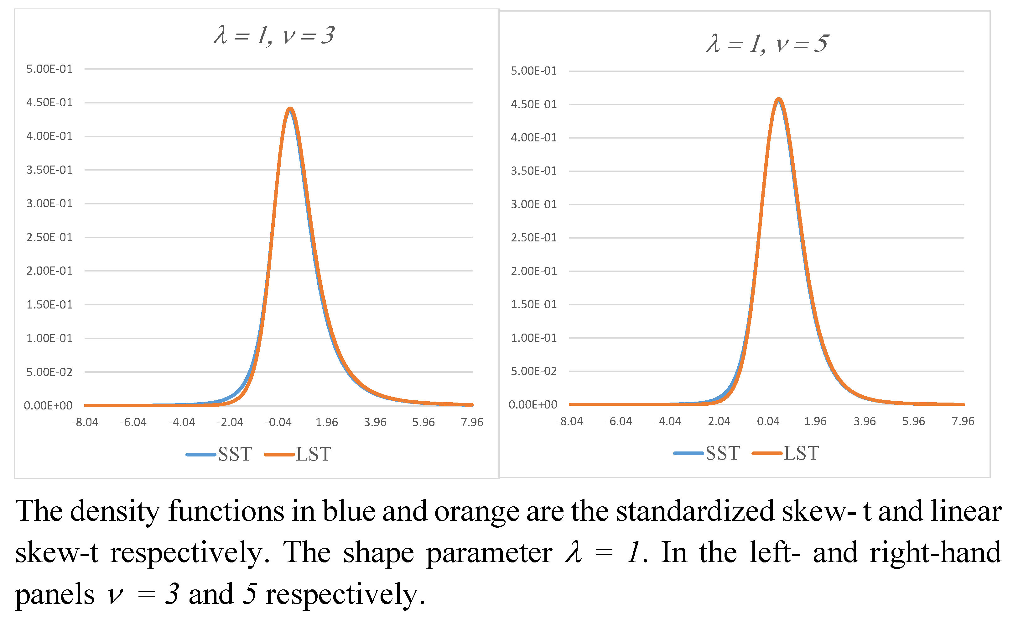
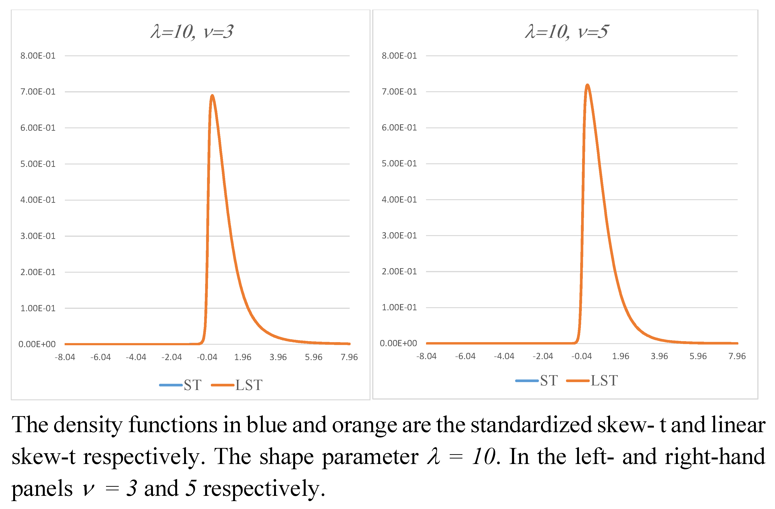
Examples of the density function with shape or skewness parameter λ set equal to 1 are shown in Figure 1. In the left- and right-hand panels, ν = 3 and 5, respectively. As the figure suggests visually, for the same value of λ , the difference between the SST and LST density functions appears to be minor, even for small degrees of freedom. Figure 2 shows the corresponding density functions for λ = 10 . As the figure shows, the distribution is not truncated as such, but the density function decays steeply for values of X less than zero.
Note that the conditional distribution of Y given X = x is Student’s t but that there is no closed-form expression for the unconditional distribution of Y.

3.2. Moments and Critical Values of the LST and SST Distributions

For ν > n and n being an odd integer, integration by parts shows that moments about the origin for the LST distribution at Equation (11) are given by the recursion
E X n = n 1 ν ν n E X n 2 + 2 λ ν ν + 1 ν n R n ν ,
where
R n ν = x n 1 1 + x 2 / ν t ν x t ν + 1 λ x ν + 1 / ν d x ,
and
E X = 2 λ ν ν + 1 ν 1 1 + x 2 / ν t ν x t ν + 1 λ x ν + 1 / ν d x .
Additional details of the result at Equation (14) are in Appendix B. Note that R n ν , and hence E X n exist for n < ν . There are no analytic expressions for the integrals in Equations (15) and (16), except for the case λ = 1 . The integrals may be computed numerically, in principle, to any specified degree of accuracy. For even values of n, the distribution of X 2 under both the SST and LST distributions is F 1 , ν ; it follows that
E X 2 = ν / ν 2 , E X 4 = 3 ν 2 / ν 2 ν 4 ,
and so on, with the usual restrictions on the maximum value of n being dependent on ν .
For fixed λ , the differences in moments and critical values decrease with increasing ν . This is illustrated in Table 1 and Table 2. These show computed values of the first four moments for both the LST and SST distributions for λ = 1 , 2 and λ = 5 , 10 , respectively, and ν = 5 , 10 , 500 and . Expressions for the SST moments are well-known, see for example [2] or, for results in notation consistent with that used in this paper, [48]. Comparative results for the critical values of these distributions are shown in Table 3 and Table 4 for a selection of percentage probabilities ranging from 1 % to 99 % . Contrary to the visual impression of the density functions in Figure 1 and Figure 2, Table 1 and Table 3 show that, for small degrees of freedom and λ = 1 , there are differences in both moments and tail behavior. The differences in critical values are more marked in the left-hand tail. The opposite would be the case if λ were equal to 1 . For a fixed value of λ , asymmetry, measured by standardized skewness, decreases as ν .

4. Extended Version of the Linear Skew-t

In standardized form, the extended skew-t distribution, SEST henceforth, has the density function
f x = t ν x T ν + 1 ν + 1 / ν + x 2 τ 1 + λ 2 + λ x / T ν τ .
The hidden truncation model corresponding to that in Section 3 has a normal distribution with conditional mean equal to
τ 1 + λ 2 + λ x 1 + x 2 / ν
and other assumptions unchanged. The linear extended skew-t distribution, LEST henceforth, corresponding to Equation (11), has the density function
f x = K t ν x T ν + 1 ν + 1 / ν τ 1 + λ 2 + λ x ,
with the normalizing constant K given by
K 1 = t ν x T ν + 1 ν + 1 / ν τ 1 + λ 2 + λ x d x = Ω ν τ , λ .
Equation (20) may be evaluated numerically. Note that Ω ν 0 , λ = 0.5 and also that
l i m ν Ω ν τ , λ = Φ τ .
For fixed values of ν and τ , as λ ± , the limiting forms of the distributions at Equations (18) and (19) are truncated t.
Proposition 2.
For fixed values of ν and τ, in Equations (18) and (19), the limiting form of the argument of the skewing function T ν + 1 . are, respectively,
ν + 1 / ν + x 2 λ x + τ ; ν + 1 / ν λ x + τ .
These take values , 0 and for x + τ greater than, equal to or less than 0, respectively. For both distributions and λ > 0 , the limiting distribution is the truncated t with density function
f x = t ν x / T ν τ ; x τ .
There is a similar result for the case λ .
For λ = 0 , the extended skew-t has the symmetric distribution reported in [9,10]. For the linear extended skew-t it is Student’s t.
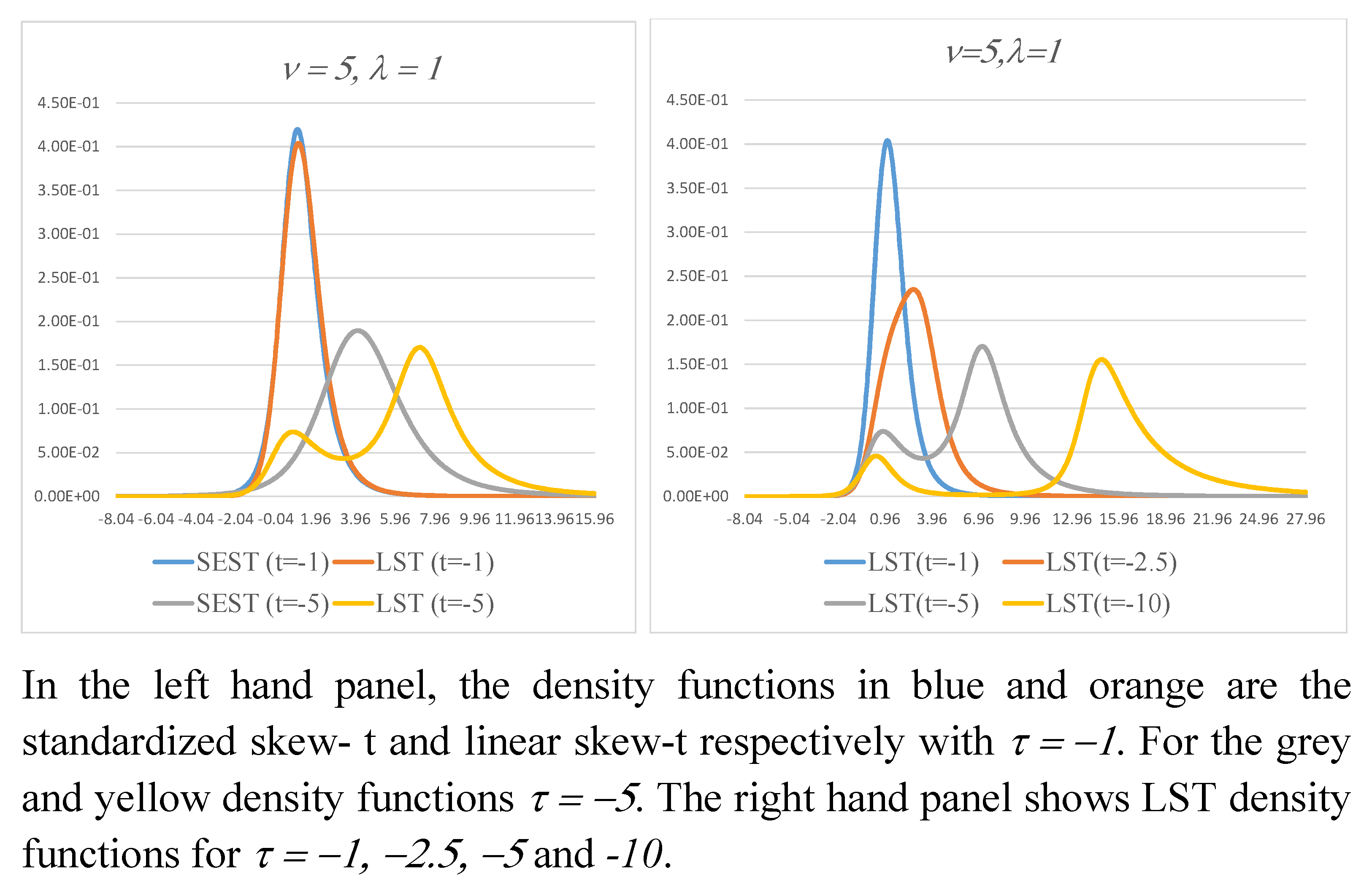
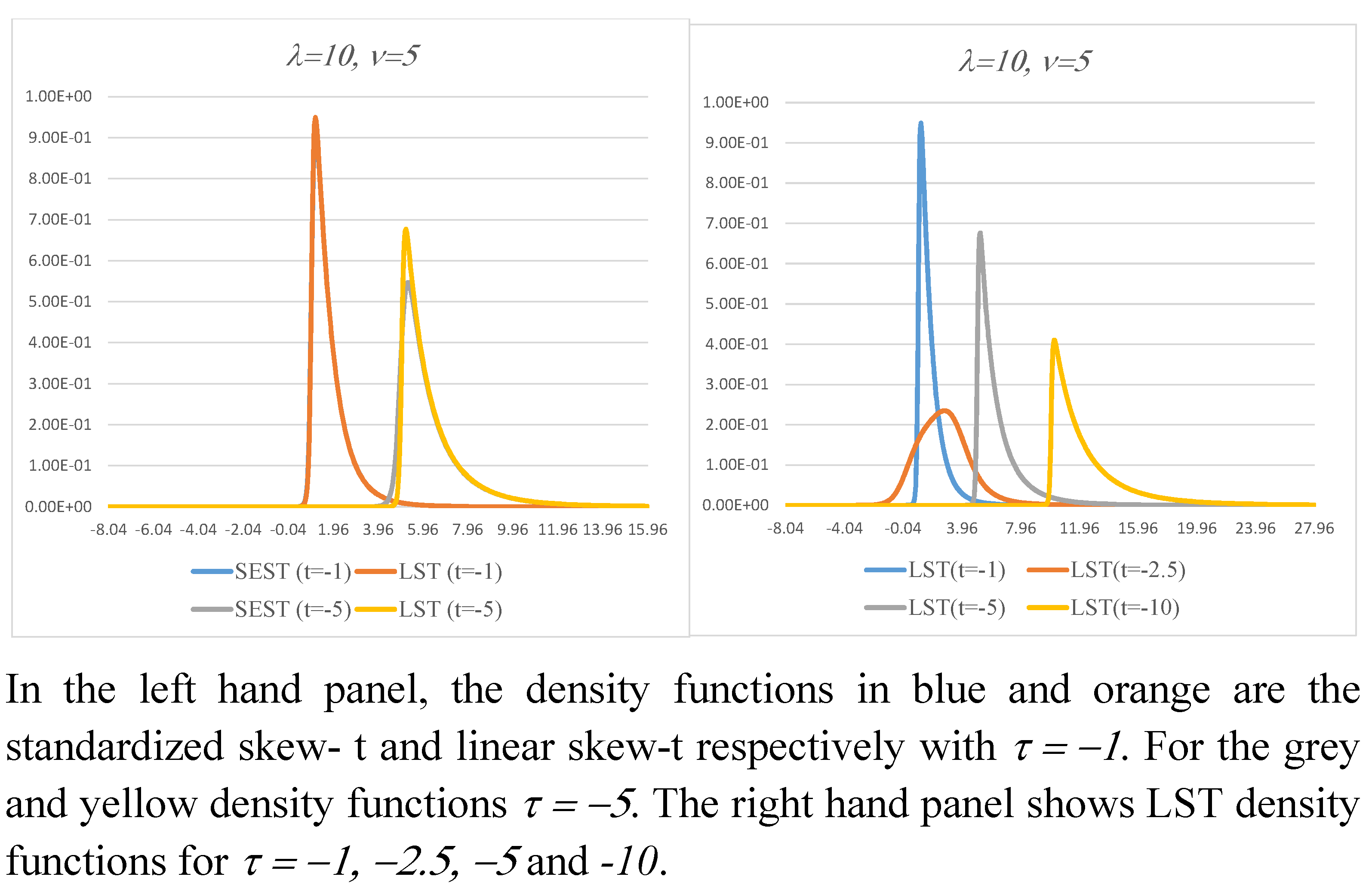
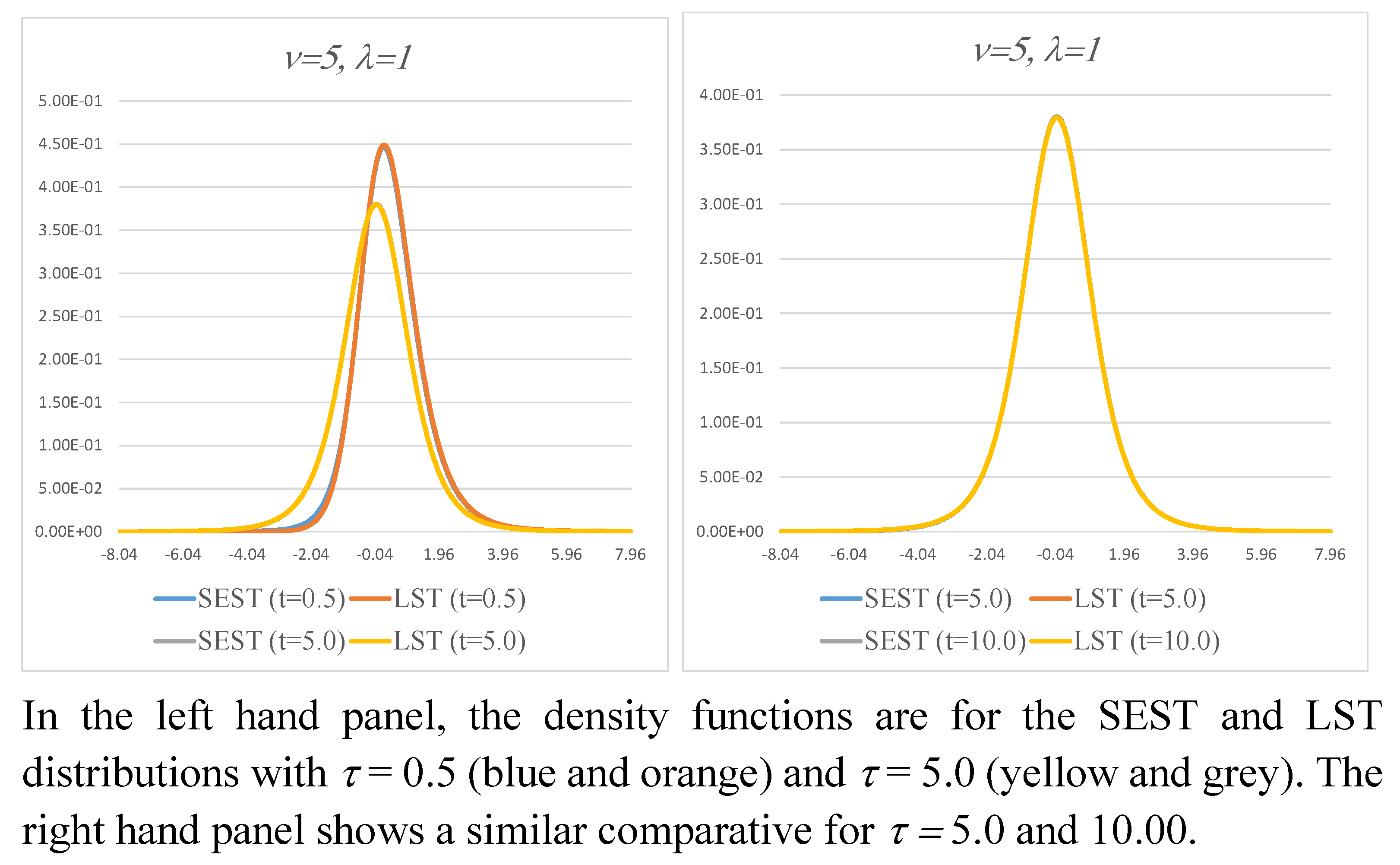
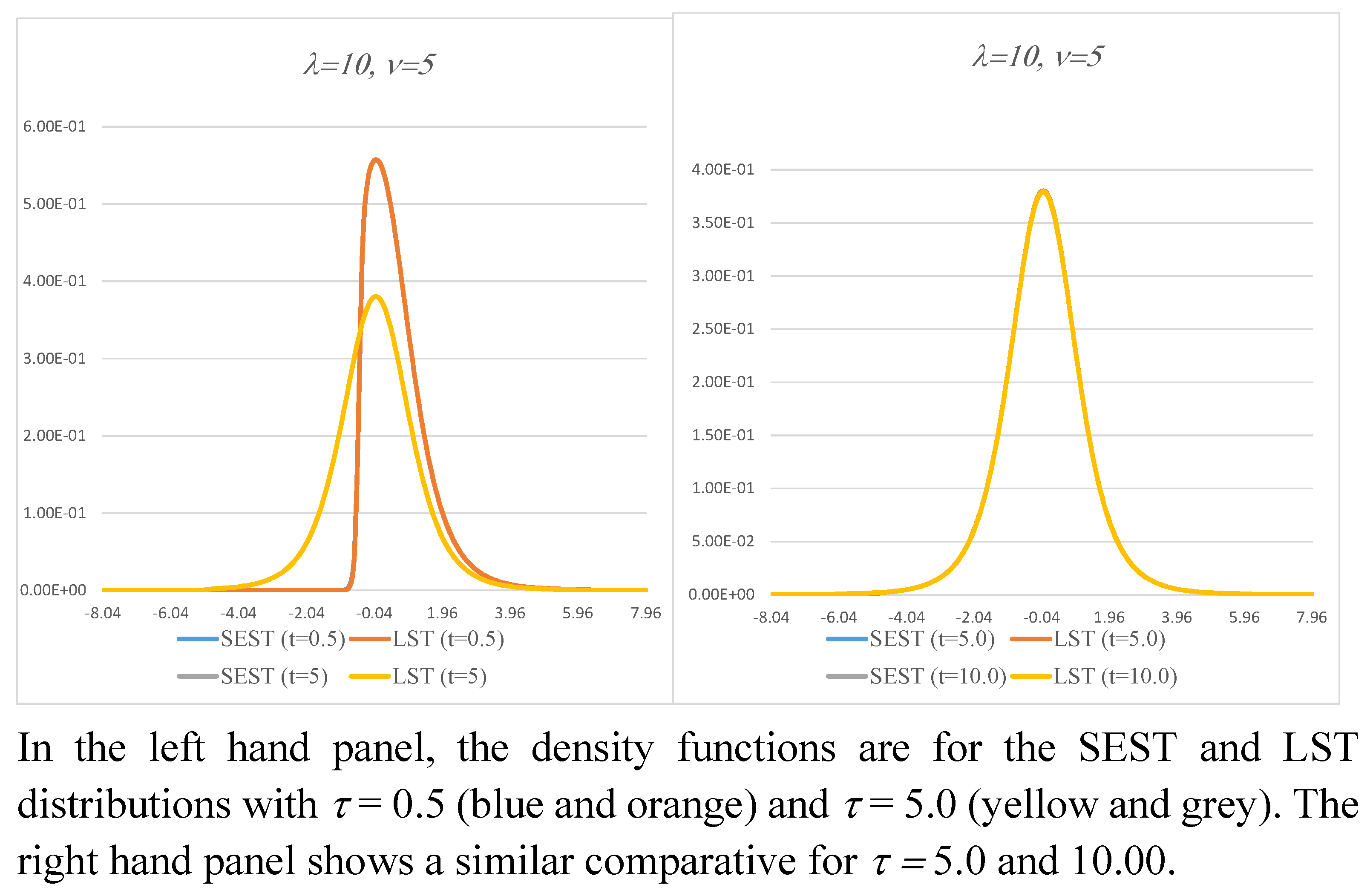
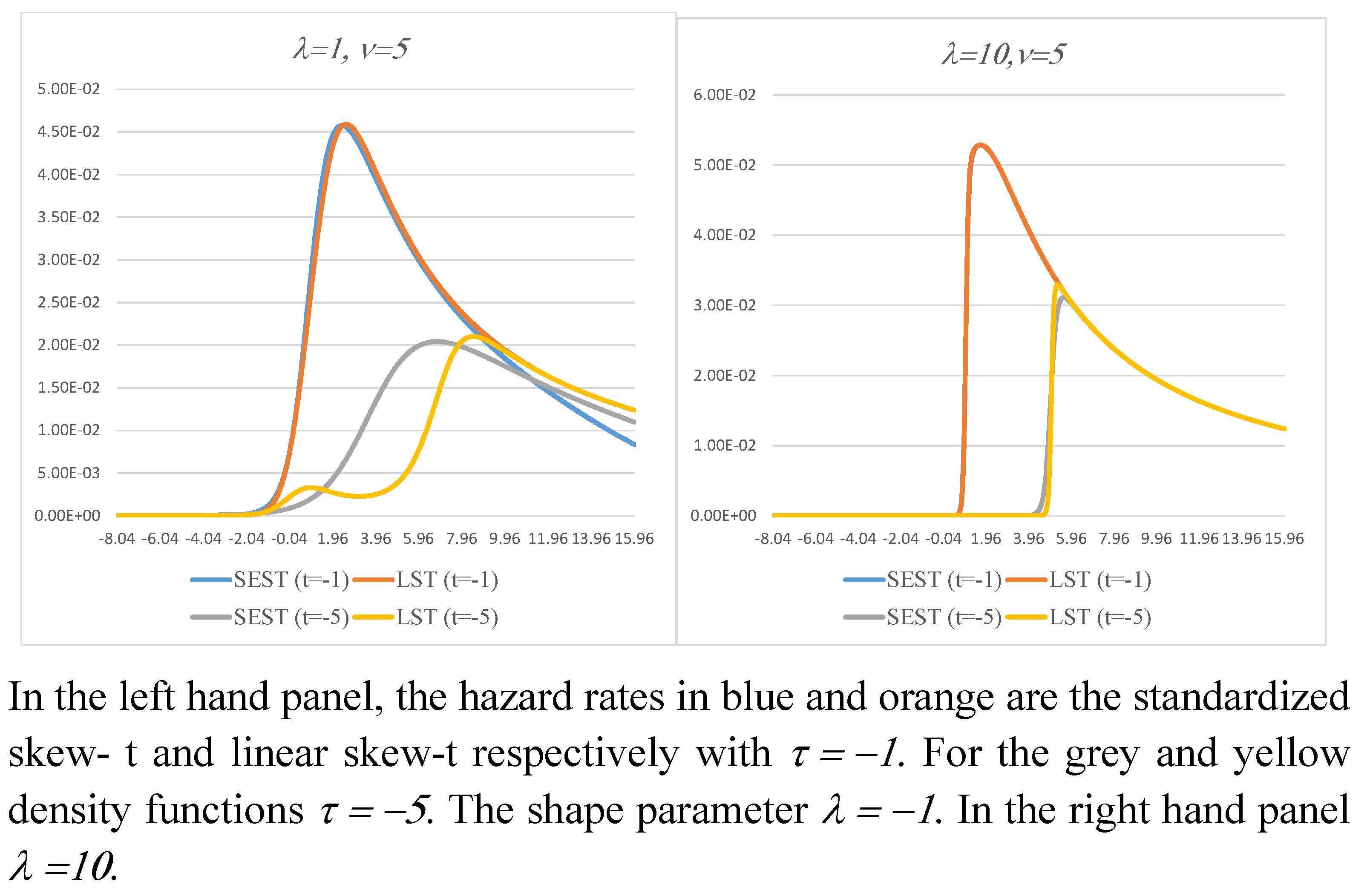
Examples of the normalizing constant Ω are shown in Table 5 for λ = 1 , 2 , 5 and 10 and a range of values of ν and τ . Note that for negative values of τ with large magnitude, the computations reported in the table use Lemma 4 reported in [48], a result originally due to [49]. Examples of the SEST and LEST density functions for ν = 5 and λ = 1 are shown in Figure 3. In the left-hand panel, τ takes values equal to 1 and 5 . For τ = 1 , both density functions are unimodal and visually similar. For τ = 5 , the two density functions differ markedly in appearance, and the LEST density function is bimodal. The right-hand panel shows LEST density functions for τ = 1 , 2.5 , 5 and 10 . As | τ | increases, the bimodality becomes more pronounced. Figure 4 shows the corresponding density functions for λ = 10 . There is no sign of bimodality. The density functions are not truncated as such, but the figure illustrates the sharp fall in density values, even for ν = 5 . Figure 5 and Figure 6 show examples of the density functions for positive values of τ . All the ones shown are unimodal, with little or no visual differences in the density functions apparent with increasing τ . The bimodality that occurs for some values of the LEST model parameters suggests that this family of distributions may be of use for applications in which the hazard rate is not monotonic. Health and employment turnover are but two examples of the presence of bimodality; see for example [50,51]. Examples of the hazard rate are shown in Figure 7.

Moments and Critical Values of the Extended Skew-t and Linear Skew-t Distributions

For the extended version of the LST distribution at Equation (18), and for n < ν , the expression corresponding to that at Equation (14) is
E X n = n 1 ν ν n E X n 2 + λ ν ν + 1 ν n Ω ν τ , λ R n ν , τ ,
with
R n ν , τ = x n 1 1 + x 2 / ν t ν x t ν + 1 ν + 1 / ν τ 1 + λ 2 + λ x d x ,
which applies for both odd and even values of n.
Moments of the SEST and LEST distributions are shown in Table 6 for λ = 1 , 2 , ν = 5 and a range of values of τ . Table 7 shows the corresponding results for λ = 5 and 10. Given the distributions shown in Figure 3 and Figure 4, the differences between the moments of the SEST and LEST distributions for negative values of τ are not surprising. Table 8 and Table 9 show the corresponding critical values. In Table 8, there are differences in the critical values of the two distributions at all given levels of probability. As implied by the result of Proposition 2, differences in the critical values decrease with increasing λ .

5. Multivariate Distributions

The references listed in Section 2 suggest that the emphasis of research has been on univariate developments, even though Lemma 1 of [4] proposes a multivariate construction. Like its skew-t counterpart, the construction of the linear skew-t leads to a multivariate form. The multivariate (and bivariate) version of the LST distribution in this paper follows the original development of the multivariate skew-normal at Equation (23) of [52], with Ω set to a unit matrix.
There is a similar result to Proposition 1 for the multivariate case that corresponds to Equation (2). As shown below, the integration involved may be simplified to some extent.
Proposition 3.
Conditional on S = s , let X N n 0 , I / s , and let Y have a normal distribution with expected value λ T x 1 + x T x / ν and variance 1 / s , S∼ χ ν 2 / ν . The result corresponding to Equation (2) is that the density function of X given that Y > 0 is
f x = 2 t n , ν x T ν + n ν + n / ν λ T x .
The proof also follows by direct verification. The details are omitted.
An extended version of the distribution at Equation (23) corresponding to Equation (19) has the density function
f x = K n t n , ν x T ν + n ν + n / ν τ 1 + λ T λ + λ T x ,
with normalizing constant K n 1 given by
. . t n , ν x T ν + n ν + n / ν τ 1 + λ T λ + λ T x d x = Ω ν , n τ , λ .
This may be reduced to the one-dimensional integral
Ω ν , n τ , λ = | Λ | 1 t ν y / | Λ | T ν + n ν + n / ν τ 1 + Λ 2 + y d y ,
with Λ 2 = λ T λ , which may be evaluated numerically. As ν , however, the limiting distribution is the standardized extended skew-normal with density function
f x = ϕ x Φ τ 1 + λ T λ + λ T x / Φ τ .
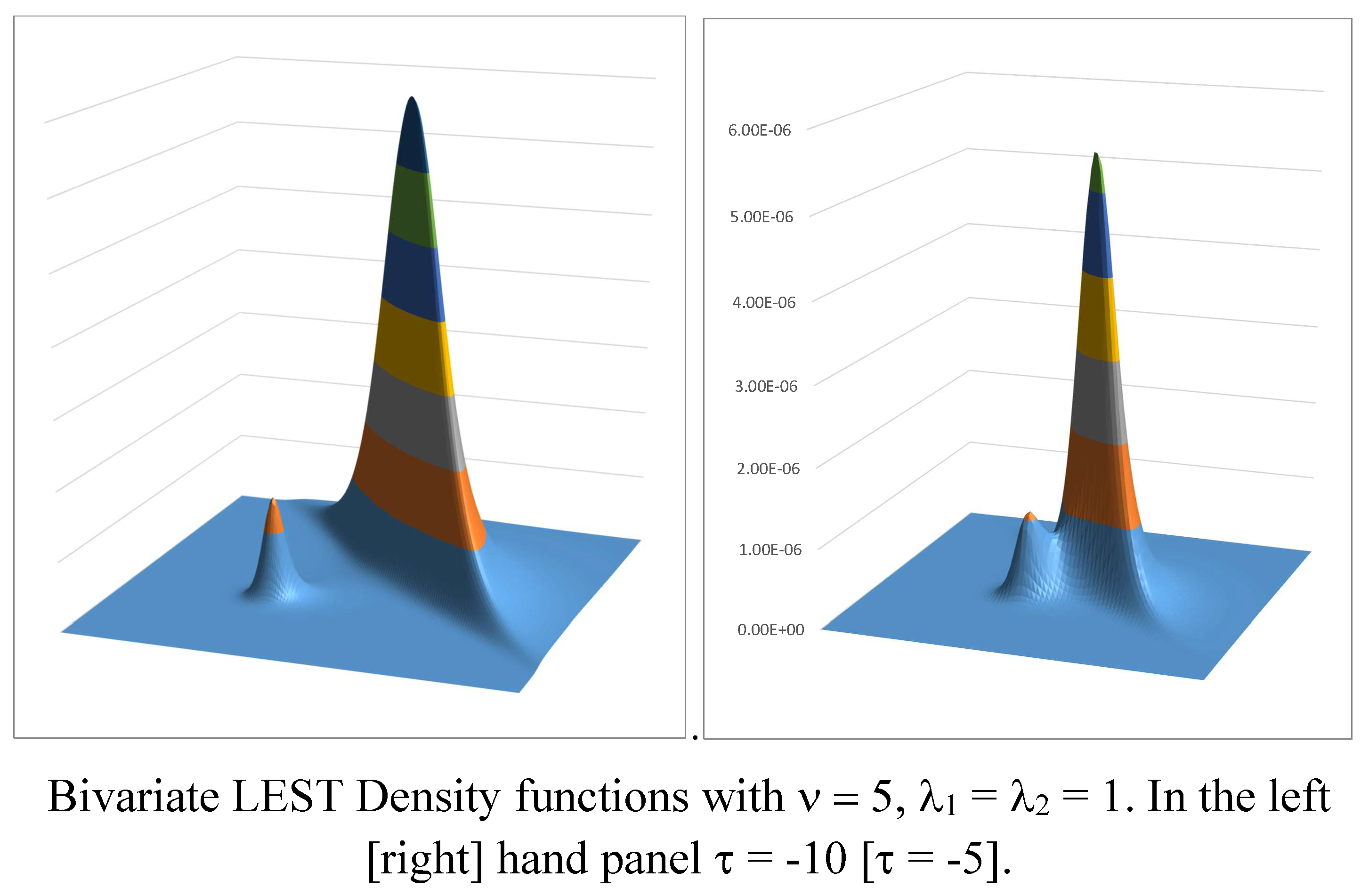
For certain negative values of τ and for small degrees of freedom, the bivariate form of the LEST distribution can be bimodal. Figure 8 shows two examples when ν = 5 , λ 1 = λ 2 = 1 and τ = 5 and 10 , respectively. These figures offer further evidence of the more complex shapes that can arise with symmetry-modulated distributions, there being other examples in Figure 1 of [2] and Figure 2 of [11].

5.1. Marginal Distributions

Let X be partitioned as X , Y T , where X is a scalar and Y an ( n 1 ) -vector. Similarly, partition the shape parameter vector as λ T = λ X , λ Y T . The density function of marginal distribution of X is given by
f x = K ν , n 1 + x 2 / ν + y T y / ν ( ν + n ) / 2 T ν + n R d y / Ω ν , n τ , λ ,
where
R = ν + n / ν τ 1 + λ X 2 + λ Y T λ Y + λ X x + λ Y T y .
This may be reduced to the one-dimensional integral
f x = K ν , n Λ Y 1 + x 2 / ν + z 2 / ν Λ Y 2 ( ν + n ) / 2 T ν + n R Z d z / Ω ν , n τ , λ ,
where Λ Y 2 = λ Y T λ Y , K ν , n is the normalizing constant for the multivariate Student distribution with ν degrees of freedom and n variables and
R Z = ν + n / ν τ 1 + λ X 2 + Λ 2 + λ X x + z .
Using integration by parts, for ν > 2 , the expected value of X may be written as the two-dimensional integral
E X = λ X Ξ K ν , n 1 + x 2 / ν + z 2 / ν Λ Y 2 ( ν + n 2 ) / 2 t ν + n R Z d z d x ,
where
Ξ = ν ( ν + n ) Ω ν , n τ , λ Λ Y ( ν + n 2 ) .
Similar expressions for E X 2 and second-order cross-moments, which require a trivariate integral, are omitted. The integrals at Equations (29) and (31) may be computed numerically. In principle, the method of Equation (29) may be used to compute the density function of the marginal distribution of a vector-valued subset of X . The expression at Equation (29) suggests that for finite values of the degrees of freedom parameter ν , the marginal distribution of the scalar variable X may not be linear skew-t. More generally, the LST distribution may not be closed under marginalization. At the time of writing, this remains a conjecture because of the need to use numerical methods to compute the integrals involved. The limiting extended skew-normal distribution is, of course, closed under marginalization.
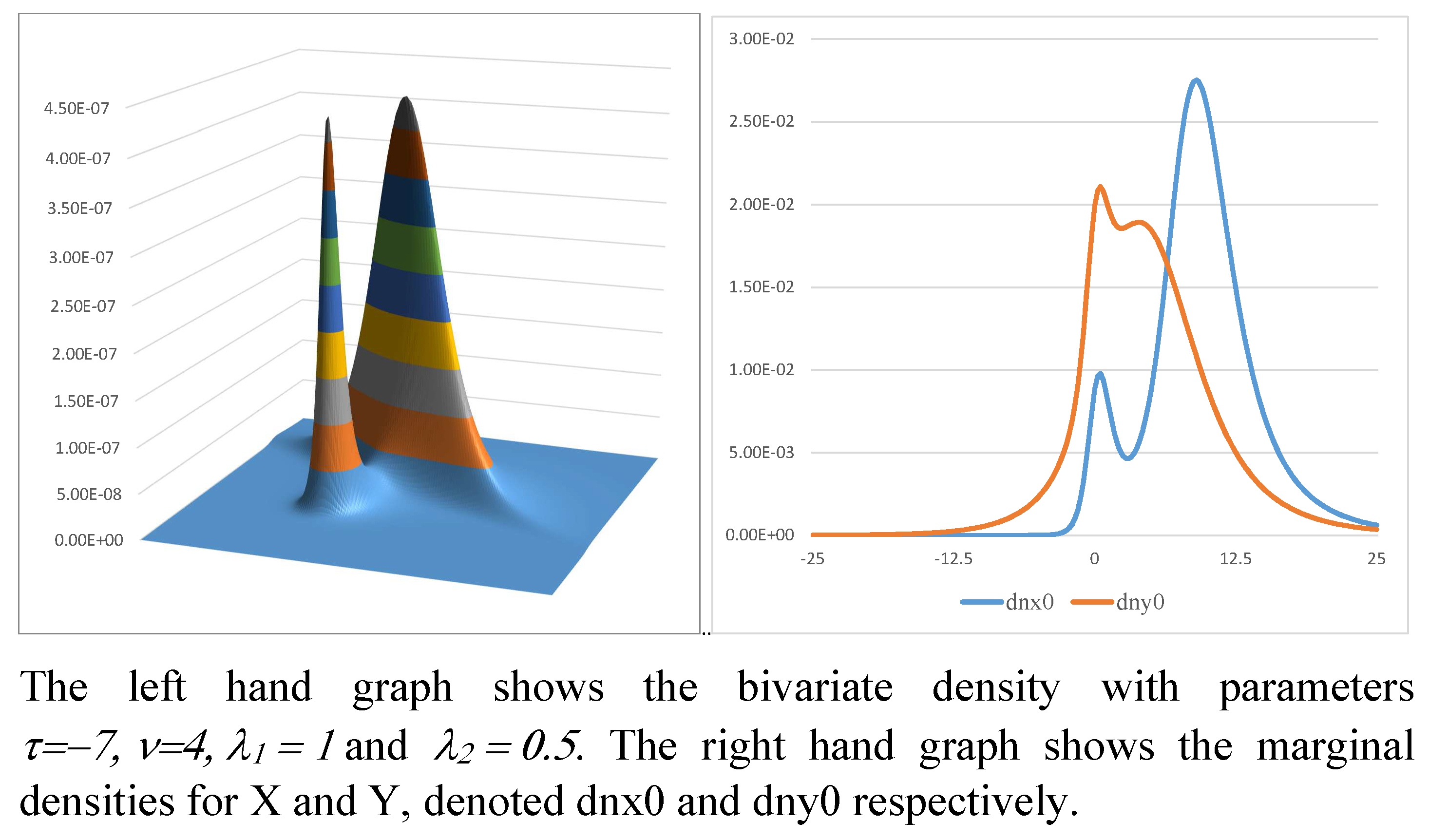
Figure 9 shows another example of a bivariate LEST distribution which is also bimodal. In this case, both marginal distributions are bimodal too.

5.2. First- and Second-Order Moments

Examples of the values of first- and second-order moments are shown in Table 10 and Table 11. These are all computed from bivariate LEST distributions. The first table reports results for ν = 5 and the second for ν = 5000 . Each table has five horizontal panels for values of τ equal to 5 , 1 , 0 , 1 and 5, respectively. The columns headed with [C] give results computed directly from the bivariate LEST distributions using numerical integration. The columns headed [ST] and [SN] contain exact results from the standardized bivariate extended skew-t (with the same degrees of freedom) and the extended skew-normal distributions. The abbreviations (1,1) and (1,2) refer to the values of the shape parameters used. In the former, λ 1 = λ 2 = 1 , and in the latter, λ 1 = 1 , λ 2 = 2 . Computations are displayed to four decimal places.
In Table 10, the computed values of the moments differ depending on the distribution. For the parameters used in the tables, the differences are more marked when τ 0 . In Table 11, as implied by the limiting distribution at Equation (26), the moments vary little depending on the distribution. As a further illustration, Table 12 and Table 13 show a selection of first- and second-order moments for the same values of τ as above, with ν = 5 and 5000 and for combinations of different values of the shape parameter λ . To save space, only values for the LEST distribution are shown. More detailed results are available on request. The results in all four tables in this section provide a demonstration of the lack of closure of the LEST distribution under marginalization.

6. Stochastic Ordering

The previous sections demonstrate that there are numerous differences between the SST and LEST distributions, although these do diminish as the degrees of freedom increase. Another area of difference is the presence or absence of stochastic ordering. This property, which is related to stochastic dominance, is satisfied by the skew-t itself. More generally, it is satisfied by distributions of the type described in [5], in particular in Section 3.1 of that paper. The result below, motivated by [53] and believed to be a new result, shows that stochastic ordering holds for the standardized extended skew-t distribution, as well as the skew-t.
Proposition 4.
Let the random variable X have the standardized extended skew-t distribution with density function at Equation (18) and denote the distribution function by F x . It follows that d F / d λ 0 , that is, stochastic ordering with respect to λ holds for nonzero values of τ.
The proof follows by direct verification, with details in Appendix C.
For the linear extended skew t, the distribution function corresponding to the density at Equation (19) is
F x = x t ν s T ν + 1 g s / Ω ν τ , λ d s ,
where
g s = ν + 1 / ν τ 1 + λ 2 + λ s ,
from which the numerator of d F x / d λ is
ν + 1 / ν x s + λ τ / 1 + λ 2 t ν s t ν + 1 g s d s F x Ω ν τ , λ / λ .
A useful algebraic representation for the LEST distribution function at Equation (33) is not available at present. Numerical computations for a range of values of ν , τ and λ are reported in Table 14. The results show the computed maximum value of the numerator of d F x / d λ , rounded to 10 decimal places. For many of the parameter combinations shown, the maxima equal zero. For numerous others, the maxima are positive. The results shown in this table demonstrate that, to 10 decimal places at least, the linear extended skew-t does not satisfy the required conditions for stochastic ordering to hold.
Note that the results in this subsection hold for nonstandardized versions of the LEST and EST distributions at Equations (18) and (19). They require modification for parameterizations in which the shape parameter λ is a component of scale.

7. Concluding Remarks and Discussion

The linear skew-t distribution is a specific form of symmetry-modulated distribution in which the two density functions used in its construction are Student’s t. Extended versions of the distribution, which give greater flexibility in both moments and critical values, are developed following the type of parameterization used for the extended skew-normal one. Parameter estimation is facilitated by the simpler argument of the skewing function T ν + 1 . . However, the stronger motivation for use of the LST or LEST distributions would arise from differences in the shape of the density function, particularly for applications for which ν is small or τ is negative and of large magnitude. For certain values of these parameters, the distribution is bimodal. This feature creates the possibility of new application areas in empirical work.
The linear skew-t distribution arises as a result of conditioning on non-negative values of an unobserved variable and a scale mixture. The conditioning employed to derive the original skew-normal and skew-t distributions is both simple and has a useful interpretation, which relates to real situations. It is hard to envisage an empirical application in which conditioning specified in Section 3 or Section 4 would have a simple interpretation. Use of the linear skew-t distributions described in this paper would be justified mainly on empirical grounds, that is, determined by the data in question.
The extra simplicity in the parameterization of the multivariate form of the distribution may be useful for some applications. However, lack of closure under marginalization or conditioning may be a limitation for some multivariate applications. As an example, suppose that the returns on all 30 constituent stocks of the Dow Jones Industrial Index are modeled using the multivariate extended skew-t, MEST. That the joint distribution of any subset of the 30 stocks is also MEST would seem to be a desirable property. Conversely, suppose that the LEST is used instead. In this case, the joint distribution of returns on a subset of the 30 stocks is not LEST.
Another difference between the EST and LEST distributions is their stochastic ordering properties with respect to the shape parameter λ . As the paper shows, the property is satisfied for the MEST distribution, but computational results indicate that it is not generally satisfied for the LEST. For applications for which stochastic ordering is an important consideration, the LEST distribution may not be a suitable choice.
From a methodological perspective, a closed version of the LEST distribution, analogous to the closed skew-normal or SUN distribution, has potential as a future research project to offer more powerful tools. The results in this paper also suggest that symmetry-modulated distributions based on other underlying density and distribution functions may offer interesting and useful insights. However, the results here serve to remind that the relative simplicity of the skew-normal, skew-t and extensions thereof may still be preferable for some applications.
Funding

This research received no external funding.

Data Availability Statement

Not applicable.

Acknowledgments

It is a pleasure to thank Adelchi Azzalini for the correspondence about stochastic ordering, which has led directly to the result in Proposition 4, the editor of Stats and the three anonymous reviewers whose constructive comments have led to many improvements in the content and presentation of the paper.

Conflicts of Interest

The author declares no conflict of interest.

Appendix A. Proposition 1

The joint density function of X and Y given S = s is
f x , y | S = s = s / 2 π e x p x 2 + y λ · x 1 + x 2 / ν 2 s / 2 .
With S χ ν 2 / ν , the joint density function of X and Y is bivariate Student, which may be written as
f x , y = f x f y | X = x = t ν x t ν + 1 y , λ x 1 + x 2 / ν , σ 2 ,
with σ 2 = ν 1 + x 2 / ν / ν + 1 . As X t ν , the distribution of λ x 1 + x 2 / ν is symmetric about zero, and so P r Y 0 = 0.5 . Hence,
f x | Y 0 = 0.5 t ν x T ν + 1 ν + 1 ν λ x .

Appendix B. Details for Equation (8)

On integration by parts, the right-hand side of Equation (14) is
κ 1 2 x n 2 1 + x 2 / ν t ν x T ν + 1 λ x ν + 1 / ν d x + κ 2 R n ν ,
where R n ν is defined by Equation (15) and
κ 1 = ν n 1 ν 1 ; κ 2 = 2 λ ν ν + 1 ν 1 .
Noting that x n 2 1 + x 2 / ν = x n 2 + x n / ν allows the above integral to be expressed as
κ 1 E x n 2 + E x n / ν .
Rearrangement gives the result.

Appendix C. Proof of Proposition 3

The distribution function of X is
F x = x t ν s T ν + 1 ν + 1 τ 1 + λ 2 + λ s ν + s 2 / T ν τ d s .
The numerator of d F / d λ is given by
x ν + 1 ν + s 2 λ τ 1 + λ 2 + s t ν s t ν + 1 ν + 1 τ 1 + λ 2 + λ s ν + s 2 d s .
The change in variable
V = ν + 1 1 + λ 2 ν + τ 2 X + λ τ 1 + λ 2 ,
and rearrangement gives
d F / d λ = 1 + τ 2 / ν t ν τ 1 + λ 2 T ν τ v r t ν + 1 r d r 0 .

References

  1. Azzalini, A. A Class of Distributions which Includes The Normal Ones. Scand. J. Stat. 1985, 12, 171–178. [Google Scholar]
  2. Azzalini, A.; Capitanio, A. Distributions Generated by Perturbation of Symmetry With Emphasis on a Multivariate Skew t Distribution. J. R. Stat. Soc. Ser. B 2003, 65, 367–389. [Google Scholar] [CrossRef]
  3. Arnold, B.C.; Beaver, R.J. Hidden Truncation Models. Sankhya Ser. A 2000, 62, 23–35. [Google Scholar]
  4. Azzalini, A.; Capitanio, A. Statistical Applications of The Multivariate Skew Normal Distribution. J. R. Stat. Soc. Ser. B 1999, 61, 579–602. [Google Scholar] [CrossRef]
  5. Azzalini, A.; Regoli, G. Some properties of skew-symmetric distributions. Ann. Inst. Stat. Math. 2012, 64, 858–879. [Google Scholar] [CrossRef] [Green Version]
  6. Azzalini, A. An overview on the progeny of the skew-normal family—A personal perspective. J. Multivar. Anal. 2022, 188, 104851. [Google Scholar] [CrossRef]
  7. Genton, M.G.; Loperfido, N.M. Generalized skew-elliptical distributions and their quadratic forms. Ann. Inst. Stat. Math. 2005, 57, 389–401. [Google Scholar] [CrossRef] [Green Version]
  8. Adcock, C.J.; Landsman, Z.; Sushi, T. Stein’s Lemma for generalized skew-elliptical random vectors. Commun. Stat.—Theory Methods 2021, 50, 3014–3029. [Google Scholar] [CrossRef]
  9. Adcock, C.J. Asset Pricing and Portfolio Selection Based on the Multivariate Extended Skew-Student-t Distribution. Ann. Oper. Res. 2010, 176, 221–234. [Google Scholar] [CrossRef] [Green Version]
  10. Arellano-Valle, R.B.; Genton, M.G. Multivariate Extended Skew-t Distributions and Related Families. Metron 2010, 68, 201–234. [Google Scholar] [CrossRef]
  11. Adcock, C.; Azzalini, A. A selective overview of skew-elliptical and related distributions and of their applications. Symmetry 2019, 12, 118. [Google Scholar] [CrossRef] [Green Version]
  12. Figueiredo, F.; Gomes, M.I. The Skew-Normal Distribution in SPC. REVSTAT—Stat. J. 2013, 11, 83–104. [Google Scholar]
  13. Sulentic, J.W.; del Olmo, A.; Marziani, P.; Martínez-Carballo, M.A.; D’Onofrio, M.; Dultzin, D.; Perea, J.; Martínez-Aldama, M.L.; Negrete, C.A.; Stirpe, G.M.; et al. What does CIVλ 1549 tell us about the physical driver of the Eigenvector quasar sequence? Astron. Astrophys. 2017, 68, A122. [Google Scholar] [CrossRef] [Green Version]
  14. Marziani, P.; Dultzin, D.; Sulentic, J.W.; Olmo, A.D.; Negrete, C.A.; Martínez-Aldama, M.L.; D’Onofrio, M.; Bon, E.; Bon, N.; Stirpe, G.M. A Main Sequence for Quasars. Front. Astron. Space Sci. 2018, 5, 6. [Google Scholar] [CrossRef] [Green Version]
  15. Marziani, P.; del Olmo, A.; Negrete, C.A.; Dultzin, D.; Vietri, E.P.G.; Martínez-Aldama, M.L.L.; D’Onofrio, M.; Bon, E.; Bon, N.; Machado, A.D.; et al. The Intermediate-ionization Lines as Virial Broadening Estimators for Population A Quasars. Astrophys. J. Suppl. Ser. 2022, 261, 30. [Google Scholar] [CrossRef]
  16. Marziani, P.; Deconto-Machado, A.; del Olmo, A. Isolating an Outflow Component in Single-Epoch Spectra of Quasars. Galaxies 2022, 10, 54. [Google Scholar] [CrossRef]
  17. Akhgari, O.; Golalizadeh, M. On Bayesian Analysis of Seemingly Unrelated Regression Model, with Skew Distribution Error. REVSTAT—Stat. J. 2020, 18, 531–551. [Google Scholar]
  18. Stein, M.L. Parametric models for distributions when interest is in extremes with an application to daily temperature. Extremes 2021, 24, 293–323. [Google Scholar] [CrossRef]
  19. Li, Y.; Sun, Y. A multi-site stochastic weather generator for high-frequency precipitation using censored skew-symmetric distribution. Spat. Stat. 2021, 41, 100474. [Google Scholar] [CrossRef]
  20. Jones, M.C. On Families of Distributions With Shape Parameters. Int. Stat. Rev. 2014, 93, 175–192. [Google Scholar] [CrossRef]
  21. Jones, M.C. Generating Distributions By Transformation Of Scale. Stat. Sin. 2014, 24, 749–771. [Google Scholar] [CrossRef] [Green Version]
  22. Fujisawa, H.; Abe, T. A family of skew distributions with mode-invariance through transformation of scale. Stat. Methodol. 2015, 25, 89–98. [Google Scholar] [CrossRef]
  23. Mulero, J.; Sordo, M.A.; de Souza, M.C.; Suárez-LLorens, A. Two stochastic dominance criteria based on tail comparisons. Appl. Stoch. Model. Bus. Ind. 2017, 33, 575–589. [Google Scholar] [CrossRef] [Green Version]
  24. Arevalillo, J.M.; Navarro, H. A stochastic ordering based on the canonical transformation of skew-normal vectors. Test 2019, 28, 475–498. [Google Scholar] [CrossRef]
  25. Jamali, D.; Amiri, M.; Jamalizadeh, A.; Balakrishnan, N. Integral stochastic ordering of the multivariate normal mean-variance and the skew-normal scale-shape mixture models. Stat. Optim. Inf. Comput. 2020, 8, 1–16. [Google Scholar] [CrossRef]
  26. Jamali, D.; Amiri, M.; Jamalizadeh, A. Comparison of the multivariate skew-normal random vectors based on the integral stochastic ordering. Commun. Stat.—Theory Methods 2021, 50, 5215–5227. [Google Scholar] [CrossRef]
  27. Pu, T.; Balakrishnan, N.; Yin, C. An Identity for Expectations and Characteristic Function of Matrix Variate Skew-normal Distribution with Applications to Associated Stochastic Orderings. Commun. Math. Stat. 2022. [Google Scholar] [CrossRef]
  28. Jones, E.; Sagawa, S.; Koh, P.W.; Kumar, A.; Liang, P. Selective Classification Can Magnify Disparities Across Groups; Archiv—Machine Learning; Department of Computer Science, Stanford University: Stanford, CA, USA, 2021. [Google Scholar]
  29. Arnold, B.C.; Beaver, R.J. The Skew Cauchy Distribution. Stat. Probab. Lett. 2000, 49, 285–290. [Google Scholar] [CrossRef]
  30. Arnold, B.C.; Gómez, H.W.; Salinas, H. On multiple constraint skewed models. Statistics 2009, 43, 279–293. [Google Scholar] [CrossRef]
  31. Gupta, A.; Chang, F.C.; Huang, W.J. Some skew-symmetric models. Random Oper. Stoch. Equ. 2002, 10, 133–140. [Google Scholar] [CrossRef]
  32. Nadarajah, S.; Kotz, S. Skew Models I. Acta Appl. Math. 2007, 98, 1–28. [Google Scholar] [CrossRef]
  33. Abramowitz, M.; Stegun, I. Handbook of Mathematical Functions; Dover Publications: Mineola, NY, USA, 1965. [Google Scholar]
  34. Kotz, S. Multivariate Distributions at a Cross-Road. In Statistical Distributions in Scientific Work; Patil, G.P., Kotz, S., Ord, J.K., Eds.; D. Reidel Publishing Co.: Dordrecht, The Netherlands, 1975. [Google Scholar]
  35. McKay, A.T. A Bessel function distribution. Biometrika 1932, 24, 39–44. [Google Scholar] [CrossRef]
  36. Nadarajah, S. A skewed Generalized t Distribution. J. Korean Stat. Soc. 2005, 34, 311–329. [Google Scholar]
  37. Bolfarine, H.; Martínez-Flórez, G.; Salinas, H.S. Bimodal symmetric-asymmetric power-normal families. Commun. Stat.—Theory Methods 2018, 47, 259–276. [Google Scholar] [CrossRef]
  38. Amiri, M.; Gómez, H.W.; Jamalizadeh, A.; Towhidi, M. Bimodal extension based on the skew-t-normal distribution. Braz. J. Probab. Stat. 2019, 33, 2–23. [Google Scholar] [CrossRef] [Green Version]
  39. Santoro, K.; Gómez, H.J.; Gallardo, D.I.; Barranco-Chamorro, I.; Gómez, H.W. The Extended Half-Skew Normal Distribution. Mathematics 2022, 10, 3740. [Google Scholar] [CrossRef]
  40. Elal-Olivero, D.; Olivares-Pacheco, J.F.; Gómez, H.W.; Bolfarine, H. A New Class of Non Negative Distributions Generated by Symmetric Distributions. Commun. Stat.—Theory Methods 2009, 38, 993–1008. [Google Scholar] [CrossRef]
  41. Gómez-Déniz, E.; Dávilá-Cárdenes, N.; Boza-Chirino, J. Modelling expenditure in tourism using the log-skew normal distribution. Curr. Issues Tour. 2022, 25, 2357–2376. [Google Scholar] [CrossRef]
  42. Naghibi, F.; Alavi, S.M.R.; Chinipardaz, R. A New Weighted Skew Normal Model. Stat. Optim. Inf. Comput. 2022, 10, 1126–1142. [Google Scholar] [CrossRef]
  43. Rao, C.R. On Discrete Distributions Arising out of Methods of Ascertainment. Sankhya Ser. A 1965, 27, 311–324. [Google Scholar]
  44. Rasekhi, M.; Chinipardaz, R.; Alavi, S.M.R. A flexible generalization of the skew normal distribution based on a weighted normal distribution. Stat. Methods Appl. 2016, 25, 375–394. [Google Scholar] [CrossRef]
  45. Hassan, M.Y.; El-Bassiouni, M.Y. Bimodal skew-symmetric normal distribution. Commun. Stat.—Theory Methods 2016, 45, 1527–1541. [Google Scholar] [CrossRef]
  46. Kwong, H.S.; Nadarajah, S. A New Robust Class of Skew Elliptical Distributions. Methodol. Comput. Appl. Probab. 2022, 24, 1669–1691. [Google Scholar] [CrossRef]
  47. Nadarajah, S.; Lyu, J. New bivariate and multivariate log-normal distributions as models for insurance data. Results Appl. Math. 2022, 14, 100246. [Google Scholar] [CrossRef]
  48. Adcock, C.J. Properties and Limiting Forms of the Multivariate Extended Skew-Normal and Skew-Student Distributions. Stats 2022, 5, 270–311. [Google Scholar] [CrossRef]
  49. Soms, A.P. An Asymptotic Expansion for the Tail Area of the t-Distribution. J. Am. Stat. Assoc. 1976, 71, 728–730. [Google Scholar] [CrossRef]
  50. Retsky, M.; Demicheli, R. Multimodal Hazard Rate for Relapse in Breast Cancer: Quality of Data and Calibration of Computer Simulation. Cancers 2014, 6, 2343–2355. [Google Scholar] [CrossRef] [Green Version]
  51. Denrell, J.; Shapira, Z. Performance Sampling and Bimodal Duration Dependence. J. Math. Sociol. 2009, 33, 38–63. [Google Scholar] [CrossRef] [Green Version]
  52. Azzalini, A.; Dalla-Valle, A. The Multivariate Skew Normal Distribution. Biometrika 1996, 83, 715–726. [Google Scholar] [CrossRef]
  53. Azzalini, A. Private Correspondence; Letter, University of Padua: Padua, Italy, 2022. [Google Scholar]
Figure 1. Standardized skew-t and linear skew-t density functions; λ = 1 , ν = 3 & 5 .
Stats 06 00024 g001
Figure 2. Standardized skew-t and linear skew-t density functions; λ = 10 , ν = 3 & 5 .
Stats 06 00024 g002
Figure 3. Standardized extended skew-t and extended linear skew-t density functions; λ = 1 , ν = 5 , τ < 0 .
Stats 06 00024 g003
Figure 4. Standardized extended skew-t and extended linear skew-t density functions; λ = 10 , ν = 5 , τ < 0 .
Stats 06 00024 g004
Figure 5. Standardized extended skew-t and extended linear skew-t density functions; λ = 1 , ν = 5 , τ > 0 .
Stats 06 00024 g005
Figure 6. Standardized extended skew-t and extended linear skew-t density functions; λ = 10 , ν = 5 , τ > 0 .
Stats 06 00024 g006
Figure 7. Hazard rates for the standardized extended skew-t and extended linear skew-t density functions; λ = 1 , 10 , ν = 5 , τ < 0 .
Stats 06 00024 g007
Figure 8. Bivariate LEST density functions: τ = 10 , 5 , λ 1 , 2 = 1 , ν = 5 .
Stats 06 00024 g008
Figure 9. Bivariate density and marginal densities: τ = 7 , λ 1 , 2 = 1 , ν = 4 .
Stats 06 00024 g009
Table 1. Comparison of Moments, λ = 1 and 2; ν = 5 , 10 , 500 and .
Panel 1: λ = 1; ν = 5 & 10
LST[5]SESTABS(DIF)%ABS(DIF)LST[10]SESTABS(DIF)%ABS(DIF)
m10.72310.67110.05207.19220.63480.61140.02333.6761
vr01.14391.21640.07256.33820.84710.87620.02913.4328
vl01.06951.10290.03343.12040.92040.93600.01571.7019
sk01.65991.44320.216713.05430.39820.34800.050212.6069
ku016.337717.63691.29927.95193.02893.29400.26518.7519
Panel 2: λ = 1; ν = 500 &
LST[500]SESTABS(DIF)%ABS(DIF)LST[]SESTABS(DIF)%ABS(DIF)
m10.56550.56500.00040.07500.56420.56420.0000NA
vr00.68430.68470.00050.07000.68170.68170.0000NA
vl00.82720.82750.00030.03500.82560.82560.0000NA
sk00.08060.08000.00060.74690.07710.07710.0000NA
ku01.43901.44190.00290.19831.42281.42280.0000NA
Panel 3: λ = 2; ν = 5 & 10
LST[5]SESTABS(DIF)%ABS(DIF)LST[10]SESTABS(DIF)%ABS(DIF)
m10.86180.84880.01301.50400.77870.77340.00530.6780
vr00.92400.94620.02222.39960.64370.65190.00821.2730
vl00.96120.97270.01151.19270.80230.80740.00510.6345
sk01.67741.64760.02981.77680.46310.45560.00741.6076
ku014.548914.79650.24771.70232.09832.14320.04492.1406
Panel 4: λ = 2; ν = 500 &
LST[500]SESTABS(DIF)%ABS(DIF)LST[]SESTABS(DIF)%ABS(DIF)
m10.71480.71470.00010.01200.71360.71360.0000NA
vr00.49310.49320.00010.02490.49070.49070.0000NA
vl00.70220.70230.00010.01250.70050.70050.0000NA
sk00.15940.15930.00010.05720.15600.15600.0000NA
ku00.80790.80840.00040.05300.79580.79580.0000NA
In each panel, the row 1 shows values of the mean. Rows 2 to 5 show, respectively, variance, standard deviation, skewness and kurtosis. The column LST has results for the LST distribution and SST for the standardized skew-t. ABS(DIF) is absolute difference and %ABS(DIF) the corresponding percentage. In each panel, the degrees of freedom are indicated for the sets of four columns in [] after LST. Table entries are computed to 4 decimal places.
Table 2. Comparison of Moments, λ = 5 and 10; ν = 5 , 10 , 500 and .
Panel 1: λ = 5; ν = 5 & 10
LST[5]SESTABS(DIF)%ABS(DIF)LST[10]SESTABS(DIF)%ABS(DIF)
m10.93140.93060.00080.08270.84810.84790.00030.0297
vr00.79920.80070.00140.17950.53060.53110.00040.0805
vl00.89400.89480.00080.08970.72850.72870.00030.0402
sk01.70211.70120.00080.04880.50890.50870.00020.0452
ku013.746913.75720.01030.07461.71571.71710.00140.0831
Panel 2: λ = 5; ν = 500 &
LST[500]SESTABS(DIF)%ABS(DIF)LST[]SESTABS(DIF)%ABS(DIF)
m10.78360.78360.00000.00040.78240.78240.0000NA
vr00.39000.39000.00000.00140.38790.38790.0000NA
vl00.62450.62450.00000.00070.62280.62280.0000NA
sk00.20900.20900.00000.00140.20560.20560.0000NA
ku00.56760.56760.00000.00210.55740.55740.0000NA
Panel 3: λ = 10; ν = 5 & 10
LST[5]SESTABS(DIF)%ABS(DIF)LST[10]SESTABS(DIF)%ABS(DIF)
m10.98350.94430.03923.98880.88060.86040.02022.2915
vr00.69930.77500.075610.81520.47460.50970.03517.4021
vl00.83630.88030.04415.26880.68890.71390.025003.6350
sk01.92391.70750.216411.24950.59050.51780.072612.3034
ku012.436413.60911.17279.42971.36091.65580.294921.671
Panel 4: λ = 10; ν = 500 &
LST[500]SESTABS(DIF)%ABS(DIF)LST[]SESTABS(DIF)%ABS(DIF)
m10.80010.79510.0050.62570.79390.79390.0000NA
vr00.36380.37180.0082.19510.36970.36970.0000NA
vl00.60320.60980.00661.09160.6080.6080.0000NA
sk00.23180.21820.01365.86500.21480.21480.0000NA
ku00.48720.53230.04529.27350.52250.52250.0000NA
In each panel, the row 1 shows values of the mean. Rows 2 to 5 show, respectively variance, standard deviation, skewness and kurtosis. The column LST has results for the LST distribution and SST for the standardized skew-t. ABS(DIF) is absolute difference and %ABS(DIF) the corresponding percentage. In each panel, the degrees of freedom are indicated for the sets of four columns in [] after LST. Table entries are computed to 4 decimal places.
Table 3. Critical Values, λ = 1 and 2; ν = 5 , 10 , 500 and .
Panel 1: λ = 1; ν = 5 & 10
CV[LST][5]CVal[SST]ABS(DIF)%ABS(DIF)CV[LST][10]CVal[SST]ABS(DIF)%ABS(DIF)
1−1.400−1.7360.33624.000−1.344−1.5120.16812.500
2.5−1.064−1.2320.16815.789−1.064−1.1200.0565.263
5−0.784−0.8960.11214.286−0.784−0.8400.0567.143
952.5202.5200.0000.0002.1842.1840.0000.000
97.53.1363.0800.0561.7862.5762.5760.0000.000
993.9763.9760.0000.0003.1363.1360.0000.000
Panel 2: λ = 1; ν = 500 &
CV[LST][500]CV[SST]ABS(DIF)%ABS(DIF)CV[LST][]CV[SST]ABS(DIF)%ABS(DIF)
1−1.288−1.2880.0000.000−1.288−1.2880.000NA
2.5−1.008−1.0080.0000.000−1.008−1.0080.000NA
5−0.784−0.7840.0000.000−0.784−0.7840.000NA
951.9041.9040.0000.0001.9041.9040.000NA
97.52.2402.2400.0000.0002.1842.1840.000NA
992.5762.5760.0000.0002.5202.5200.000NA
Panel 3: λ = 2; ν = 5 & 10
CV[LST][5]CV[SST]ABS(DIF)%ABS(DIF)CV[LST][10]CV[SST]ABS(DIF)%ABS(DIF)
1−0.784−0.8960.11214.286−0.784−0.7840.0000.000
2.5−0.560−0.6160.05610.000−0.560−0.5600.0000.000
5−0.392−0.3920.0000.000−0.392−0.3920.0000.000
952.5202.5200.0000.0002.1842.1840.0000.000
97.53.1363.1360.0000.0002.6322.6320.0000.000
994.0323.9760.0561.3893.1363.1360.0000.000
Panel 4: λ = 2; ν = 500 &
CV[LST][500]CV[SST]ABS(DIF)%ABS(DIF)CV[LST][]CV[SST]ABS(DIF)%ABS(DIF)
1−0.728−0.7280.0000.000−0.728−0.7280.000NA
2.5−0.560−0.5600.0000.000−0.560−0.5600.000NA
5−0.336−0.3360.0000.000−0.336−0.3360.000NA
951.9601.9600.0000.0001.9601.9600.000NA
97.52.2402.2400.0000.0002.2402.2400.000NA
992.5762.5760.0000.0002.5762.5760.000NA
Critical values are shown for a selection of percentage probabilities ranging from 1% to 99%. The column CV[LST] has results for the LST distribution and CV[SST] for the standardized skew-t. ABS(DIF) is absolute difference and %ABS(DIF) the corresponding percentage. In each panel, the degrees of freedom are indicated for the sets of four columns in [] after CV[LST]. Table entries are computed to 3 decimal places.
Table 4. Critical Values, λ = 5 and 10; ν = 5 , 10 , 500 and .
Panel 1: λ = 5; ν = 5 & 10
CV[LST][5]CV[SST]ABS(DIF)%ABS(DIF)CV[LST][10]CV[SST]ABS(DIF)%ABS(DIF)
1−0.300−0.3000.0000.000−0.300−0.3000.0000.000
2.5−0.200−0.2000.0000.000−0.200−0.2000.0000.000
5−0.100−0.1000.0000.000−0.100−0.1000.0000.000
952.5002.5000.0000.0002.2002.2000.0000.000
97.53.1003.1000.0000.0002.6002.6000.0000.000
994.0004.0000.0000.0003.1003.1000.0000.000
Panel 2: λ = 5 ; ν = 500 &
CV[LST][500]CV[SST]ABS(DIF)%ABS(DIF)CV[LST][]CV[SST]ABS(DIF)%ABS(DIF)
1−0.300−0.3000.0000.000−0.300−0.3000.000NA
2.5−0.200−0.2000.0000.000−0.200−0.2000.000NA
5−0.100−0.1000.0000.000−0.100−0.1000.000NA
951.9001.9000.0000.0001.9001.9000.000NA
97.52.2002.2000.0000.0002.2002.2000.000NA
992.5002.5000.0000.0002.5002.5000.000NA
Panel 3: λ = 10; ν = 5 & 10
CV[LST][5]CV[SST]ABS(DIF)%ABS(DIF)CV[LST][10]CV[SST]ABS(DIF)%ABS(DIF)
1−0.183−0.1830.0000.000−0.183−0.1830.0000.000
2.5−0.183−0.1830.0000.000−0.183−0.1830.0000.000
50.0000.0000.000NA0.0000.0000.000NaN
952.5672.5670.0000.0002.2002.2000.0000.000
97.53.1173.1170.0000.0002.5672.5670.0000.000
994.0334.0330.0000.0003.1173.1170.0000.000
Panel 4: λ = 10; ν = 500 &
CV[LST][500]CV[SST]ABS(DIF)%ABS(DIF)CV[LST][]CV[SST]ABS(DIF)%ABS(DIF)
1−0.183−0.1830.0000.000−0.183−0.1830.000NA
2.5−0.183−0.1830.0000.000−0.183−0.1830.000NA
50.0000.0000.000NA0.0000.0000.000NA
951.8331.8330.0000.0001.8331.8330.000NA
97.52.2002.2000.0000.0002.2002.2000.000NA
992.5672.5670.0000.0002.5672.5670.000NA
Critical values are shown for a selection of percentage probabilities ranging from 1% to 99%. The column CV[LST] has results for the LST distribution and CV[SST] for the standardized skew-t. ABS(DIF) is absolute difference and %ABS(DIF) the corresponding percentage. In each panel, the degrees of freedom are indicated for the sets of four columns in [] after CV[LST]. Table entries are computed to 3 decimal places.
Table 5. Normalizing Constant for the Extended LST Distribution, λ = 1, 2, 5 and 10.
Panel 1: λ = 1
ν = / τ = −10−5−1−0.500.51510
50.00000.00080.1820.32170.50000.67830.8180.99921.0000
70.00000.00030.17560.31820.50000.68180.82440.99971.0000
100.00000.00010.17060.31540.50000.68460.82940.99991.0000
250.00000.00000.16350.31140.50000.68860.83651.00001.0000
500.00000.00000.16110.31000.50000.69000.83891.00001.0000
1000.00000.00000.15990.30920.50000.69080.84011.00001.0000
5000.00000.00000.15890.30870.50000.69130.84111.00001.0000
10000.00000.00000.15880.30860.50000.69140.84121.00001.0000
50000.00000.00000.15870.30860.50000.69140.84131.00001.0000
Inf0.00000.00000.15870.30850.50000.69150.84131.00001.0000
Panel 2: λ = 2
ν = / τ = −10−5−1−0.500.51510
50.00010.00150.18440.32270.50000.67730.81560.99850.9999
70.00000.00050.17740.31890.50000.68110.82260.99951.0000
100.00000.00020.17190.31590.50000.68410.82810.99981.0000
250.00000.00000.1640.31150.50000.68850.8361.00001.0000
500.00000.00000.16140.31010.50000.68990.83861.00001.0000
1000.00000.00000.16000.30930.50000.69070.84001.00001.0000
5000.00000.00000.15890.30870.50000.69130.84111.00001.0000
10000.00000.00000.15880.30860.50000.69140.84121.00001.0000
50000.00000.00000.15870.30860.50000.69140.84131.00001.0000
Inf0.00000.00000.15870.30850.50000.69150.84131.00001.0000
Panel 3: λ = 5
ν = / τ = −10−5−1−0.500.51510
50.00010.00190.18250.32030.50000.67970.81750.99810.9999
70.00000.00070.1760.3170.50000.6830.8240.99931.0000
100.00000.00020.17090.31450.50000.68550.82910.99981.0000
250.00000.00000.16360.31090.50000.68910.83641.00001.0000
500.00000.00000.16110.30970.50000.69030.83891.00001.0000
1000.00000.00000.15990.30910.50000.69090.84011.00001.0000
5000.00000.00000.15890.30870.50000.69130.84111.00001.0000
10000.00000.00000.15880.30860.50000.69140.84121.00001.0000
50000.00000.00000.15870.30850.50000.69150.84131.00001.0000
Inf0.00000.00000.15870.30850.50000.69150.84131.00001.0000
Panel 4: λ = 10,
ν = / τ = −10−5−1−0.500.51510
50.00010.00200.18180.31990.50000.68010.81820.99800.9999
70.00000.00080.17540.31670.50000.68330.82460.99921.0000
100.00000.00030.17050.31430.50000.68570.82950.99971.0000
250.00000.00000.16350.31090.50000.68910.83651.00001.0000
500.00000.00000.16110.30980.50000.69020.83891.00001.0000
1000.00000.00000.15990.30920.50000.69080.84011.00001.0000
5000.00000.00000.15890.30870.50000.69130.84111.00001.0000
10000.00000.00000.15880.30870.50000.69130.84121.00001.0000
50000.00000.00000.15870.30860.50000.69140.84131.00001.0000
Inf0.00000.00000.15870.30850.50000.69150.84131.00001.0000
The table displays values of the normalizing constants Ω ν τ , λ as defined at Equation (20), computed numerically and displayed to 4 decimal places. Note that for negative values of t with large magnitude, the computations use Lemma 4 of [48], a result originally due to [49].
Table 6. Moments of the Extended Distributions, λ = 1 and 2; ν = 5.
Panel 1: λ = 1, : τ = 10 & 5
LST[−10]SSTABS(DIF)%ABS(DIF)LST[−5]SSTABS(DIF)%ABS(DIF)
m114.89378.90145.992440.23416.14144.54121.600226.0556
vr051.101727.335723.765946.507213.69167.80345.888243.0061
vl07.14855.22841.920226.86123.70022.79340.906824.5057
sk0125.9908178.097252.106541.357434.833727.09837.735422.2066
ku036,857.72312,883.421223,974.301865.04552010.39591031.9234978.472648.6706
Panel 2: λ = 1, : τ = 1 & 1
LST[−1]SSTABS(DIF)%ABS(DIF)LST[1]SSTABS(DIF)%ABS(DIF)
m11.37161.28300.08866.46200.30520.28470.02056.7223
vr01.46761.53260.06504.42941.19911.25010.05094.2477
vl01.21141.23800.02652.19071.0951.11810.0232.1018
sk02.61182.25310.358713.73321.37281.18690.186013.5455
ku031.294633.69382.39937.666713.581114.57820.99717.3422
Panel 3: λ = 1, : τ = 5 & 10
LST[5]SSTABS(DIF)%ABS(DIF)LST[10]SSTABS(DIF)%ABS(DIF)
m10.00520.00930.004280.97560.00030.00080.0005150.7225
vr01.62481.61150.01330.81831.66111.65770.00340.2071
vl01.27471.26950.00520.41001.28891.28750.00130.1036
sk00.41070.42180.01112.70030.11490.13410.019216.7355
ku018.804919.03980.23491.249121.707921.71080.0030.0136
Panel 4: λ = 2, : τ = 10 & 5
LST[−10]SSTABS(DIF)%ABS(DIF)LST[−5]SSTABS(DIF)%ABS(DIF)
m113.823611.25952.564118.54886.72125.74420.976914.5353
vr014.511317.56033.049021.01134.58665.06310.476510.3892
vl03.80944.19050.381110.00512.14162.25010.10855.0662
sk0220.6985180.638040.060418.151630.408627.65442.75429.0573
ku013,283.594510,006.64663276.947924.6691974.6452804.9936169.651617.4065
Panel 5: λ = 2, : τ = 1 & 1
LST[−1]SSTABS(DIF)%ABS(DIF)LST[1]SSTABS(DIF)%ABS(DIF)
m11.64321.62290.02031.23810.37160.36010.01153.0961
vr01.05851.08930.03072.90261.05541.08060.02522.3924
vl01.02891.04370.01481.44091.02731.03950.01221.1891
sk02.4102.43180.02180.90581.50071.45080.05003.3304
ku026.513327.30410.79082.982812.422912.67880.2562.0605
Panel 6: λ = 2, : τ = 5 & 10
LST[5]SSTABS(DIF)%ABS(DIF)LST[10]SSTABS(DIF)%ABS(DIF)
m10.00980.01180.00220.71450.00070.0010.000233.8465
vr01.59651.59170.00490.30451.65611.65450.00160.0959
vl01.26351.26160.00190.15241.28691.28630.00060.0479
sk00.57420.56970.00440.77460.17660.18340.00683.829
ku017.62217.76020.13820.784220.910020.93500.02490.1193
kp49.975210.15990.18471.851612.682412.72310.04070.321
In each panel, the rows 1 to 5 show, respectively, mean, variance, standard deviation, skewness and kurtosis. The column LST has results for the LEST distribution and SST for the SEST. ABS(DIF) is absolute difference and %ABS(DIF) the corresponding percentage. In each panel, the values of t are indicated for the sets of four columns in [] after LST. Table entries are computed to 4 decimal places.
Table 7. Moments of the Extended Distributions, λ = 5 and 10; ν = 5.
Panel 1: λ = 5, : τ = 10 & 5
LST[−10]SSTABS(DIF)%ABS(DIF)LST[−5]SSTABS(DIF)%ABS(DIF)
m112.804512.3440.46053.59656.48956.29750.19192.9571
vr011.496512.29660.80016.95983.38173.58760.20596.0888
vl03.39063.50670.11603.42141.83891.89410.05522.9994
sk0177.8159171.68596.13013.447427.006826.40870.59812.2146
ku09433.2698980.1021453.1674.8039747.4836723.886123.59753.1569
kp49036.76298526.4832510.27975.6467713.1762685.273727.90253.9124
Panel 2: λ = 5, : τ = 1 & 1
LST[−1]SSTABS(DIF)%ABS(DIF)LST[1]SSTABS(DIF)%ABS(DIF)
m11.78081.77920.00160.08770.39760.39480.00280.7105
vr00.84230.85050.00820.97940.98450.98940.00490.4985
vl00.91780.92230.00450.48850.99220.99470.00250.249
sk02.40892.41920.01030.42781.56641.56070.00570.3655
ku024.842324.99290.15060.606211.928911.95780.0290.2429
kp422.713922.82260.10870.47869.02119.02100.00010.001
Panel 3: λ = 5, : τ = 5 & 10
LST[5]SSTABS(DIF)%ABS(DIF)LST[10]SSTABS(DIF)%ABS(DIF)
m10.01250.01300.00043.34120.0010.00110.00015.2119
vr01.58191.58100.00090.05571.65311.65270.00030.0195
vl01.25771.25740.00040.02791.28571.28560.00010.0097
sk00.64760.64590.00170.26190.20800.20920.00120.5656
ku017.141617.16920.02750.160620.557620.56330.00560.0274
kp49.63479.67060.03590.372412.359912.36870.00880.0715
Panel 4: λ = 10, : τ = 10 & 5
LST[−10]SSTABS(DIF)%ABS(DIF)LST[−5]SSTABS(DIF)%ABS(DIF)
m112.817312.52600.29132.27296.24136.39040.14902.3881
vr09.159111.36602.206824.09454.42103.32671.094324.7521
vl03.02643.37130.344911.39772.10261.82390.278713.2544
sk0196.4190169.489226.929813.710419.037826.09667.058937.0782
ku08596.58358836.6541240.07062.7926772.9518712.537960.41397.816
kp48344.91538449.0992104.18391.2485714.316679.336934.97914.8969
Panel 5: λ = 10, : τ = 1 & 1
LST[−1]SSTABS(DIF)%ABS(DIF)LST[1]SSTABS(DIF)%ABS(DIF)
m11.73451.80540.07104.09200.38540.40060.01533.9642
vr00.95920.80830.150815.72421.00690.97330.03373.3433
vl00.97940.89910.08038.19811.00350.98650.01691.6859
sk01.94582.41060.464823.88701.47921.57830.09916.7027
ku026.771424.66652.10497.862612.550211.85230.69785.5604
kp424.011422.70621.30525.43579.50849.01050.49785.2359
ssk02.07143.31681.245560.12951.46391.64380.179912.2865
sku029.099837.75028.650529.727012.377712.51210.13441.0858
Panel 6: λ = 10, : τ = 5 & 10
LST[5]SSTABS(DIF)%ABS(DIF)LST[10]SSTABS(DIF)%ABS(DIF)
m10.01260.01310.00054.11220.00110.00110.00000.1365
vr01.58221.57910.00310.19311.65231.65240.00010.0078
vl01.25781.25660.00120.09661.28541.28550.00000.0039
sk00.63770.65930.02153.37540.21670.21370.00301.3992
ku017.333317.07180.26151.508820.426720.50090.07420.3633
kp49.82379.59120.23252.367212.236512.30940.07290.5961
ssk00.32050.33220.01183.67560.10200.10060.00141.4107
sku06.92456.84640.07811.12737.48217.50810.02600.3478
In each panel, the rows 1 to 5 show, respectively, mean, variance, standard deviation, skewness and kurtosis. The column LST has results for the LEST distribution and SST for the SEST. ABS(DIF) is absolute difference and %ABS(DIF) the corresponding percentage. In each panel, the values of t are indicated for the sets of four columns in [] after LST. Table entries are computed to 4 decimal places.
Table 8. Critical Values of the Extended Distributions, λ = 1 and 2; ν = 5.
Panel 1: λ = 1, : λ = 10 & 5
%PrLST[−10]SSTABS(DIF)%ABS(DIF)LST[−5]SSTABS(DIF)%ABS(DIF)
1−1.064−2.6881.624152.6316−0.896−1.6240.72881.250
2.5−0.448−0.1680.28062.500−0.392−0.3360.05614.286
50.1681.6241.456866.6670.1120.6160.504450.000
9524.64017.4727.16829.09111.5369.1282.40820.874
97.528.33620.3847.95228.06313.32810.6962.63219.748
9934.04824.8649.18426.97416.07213.0483.02418.815S
Panel 2: λ = 1, : τ = 1 & 1
%PrLST[−1]SSTABS(DIF)%ABS(DIF)LST[1]SSTABS(DIF)%ABS(DIF)
1−1.008−1.4000.39238.889−1.960−2.1840.22411.429
2.5−0.616−0.8400.22436.364−1.568−1.7360.16810.714
5−0.336−0.4480.11233.333−1.288−1.3440.0564.348
953.4163.3040.1123.2792.1282.1280.0000.000
97.54.0884.0320.0561.3702.6882.6880.0000.000
995.0965.0400.0561.0993.5283.5280.0000.000
Panel 3: λ = 1, : τ = 5 & 10
%PrLST[5]SSTABS(DIF)%ABS(DIF)LST[10]SSTABS(DIF)%ABS(DIF)
1−3.360−3.2480.1123.333−3.416−3.3600.0561.639
2.5−2.576−2.5200.0562.174−2.576−2.5760.0000.000
5−2.016−2.0160.0000.000−2.016−2.0160.0000.000
952.0162.0160.0000.0001.9601.9600.0000.000
97.52.5202.5200.0000.0002.5202.5200.0000.000
993.3603.3600.0000.0003.3603.3600.0000.000
Panel 4: λ = 2, : τ = 10 & -5
%PrLST[−10]SSTABS(DIF)%ABS(DIF)LST[−5]SSTABS(DIF)%ABS(DIF)
19.8003.5846.21663.4292.0721.6240.44821.622
2.510.4165.0965.32051.0753.8082.4081.40036.765
510.7526.1044.64843.2294.5362.9681.56834.568
9520.38418.3122.07210.16510.3049.5200.7847.609
97.523.46421.1682.2969.78511.92811.0320.8967.512
9928.22425.4802.7449.72214.39213.3841.0087.004
Panel 5: λ = 2, : τ = 1 & 1
%PrLST[−1]SSTABS(DIF)%ABS(DIF)LST[1]SSTABS(DIF)%ABS(DIF)
1−0.168−0.2800.11266.667−1.456−1.6240.16811.539
2.50.1120.0560.05650.000−1.232−1.2880.0564.546
50.3360.3360.0000.000−1.008−1.0640.0565.556
953.4163.4160.0000.0002.1282.1280.0000.000
97.54.0884.0880.0000.0002.6882.6880.0000.000
995.0965.0960.0000.0003.5283.5280.0000.000
Panel 6: λ = 2, : τ = 5 & 10
%PrLST[5]SSTABS(DIF)%ABS(DIF)LST[10]SSTABS(DIF)%ABS(DIF)
1−3.248−3.2480.0000.000−3.416−3.360.0561.639
2.5−2.576−2.520.0562.174−2.576−2.5760.0000.000
5−2.016−2.0160.0000.000−2.016−2.0160.0000.000
952.0162.0160.0000.0001.9601.9600.0000.000
97.52.5202.5200.0000.0002.5202.5200.0000.000
993.3603.3600.0000.0003.3603.3600.0000.000
Critical values are shown for a selection of percentage probabilities ranging from 1% to 99%. The column LST has results for the LEST distribution and SST for the SEST. ABS(DIF) is absolute difference and %ABS(DIF) the corresponding percentage. Table entries are computed to 3 decimal places.
Table 9. Critical Values of the Extended Distributions, λ = 5 and 10; ν = 5.
Panel 1: λ = 5, : λ = 10 & 5
%PrLST[−10]SSTABS(DIF)%ABS(DIF)LST[−5]SSTABS(DIF)%ABS(DIF)
19.9008.0001.90019.1924.7003.9000.80017.021
2.510.1008.5001.60015.8424.8004.2000.60012.500
510.2009.0001.20011.7655.0004.50000.50010.000
9518.80018.4000.4002.1289.7009.6000.1001.031
97.521.60021.2000.4001.85211.20011.1000.1000.893
9926.00025.5000.5001.92313.50013.4000.1000.741
Panel 2: λ = 5, : τ = 1 & 1
%PrLST[−1]SSTABS(DIF)%ABS(DIF)LST[1]SSTABS(DIF)%ABS(DIF)
2.50.7000.7000.0000.000−1.000−1.0000.0000.000
50.8000.8000.0000.000−0.900−0.9000.0000.000
953.4003.4000.0000.0002.1002.1000.0000.000
97.54.1004.1000.0000.0002.7002.7000.0000.000
995.1005.1000.0000.0003.5003.5000.0000.000
Panel 3: λ = 5, : τ = 5 & 10
%PrLST[5]SSTABS(DIF)%ABS(DIF)LST[10]SSTABS(DIF)%ABS(DIF)
1−3.300−3.2000.1003.030−3.400−3.4000.0000.000
2.5−2.600−2.6000.0000.000−2.600−2.6000.0000.000
5−2.000−2.0000.0000.000−2.100−2.1000.0000.000
952.0002.0000.0000.0002.0002.0000.0000.000
97.52.5002.5000.0000.0002.5002.5000.0000.000
993.3003.3000.0000.0003.3003.3000.0000.000
Panel 4: λ = 10, : τ = 10 & -5
%PrLST[−10]SSTABS(DIF)%ABS(DIF)LST[−5]SSTABS(DIF)%ABS(DIF)
19.9009.1670.7337.4074.7674.5830.1833.846
2.59.9009.3500.5505.5564.9504.5830.3677.407
510.0839.7170.3673.6364.9504.7670.1833.704
9518.51718.3330.1830.9909.5339.5330.0000.000
97.521.26721.0830.1830.86211.00011.0000.0000.000
9925.66725.4830.1830.71413.38313.3830.0000.000
Panel 5: λ = 10, : τ = 1 & 1
%PrLST[−1]SSTABS(DIF)%ABS(DIF)LST[1]SSTABS(DIF)%ABS(DIF)
10.7330.7330.0000.000−1.100−1.1000.0000.000
2.50.7330.7330.0000.000−1.100−1.1000.0000.000
50.9170.9170.0000.000−0.917−0.9170.0000.000
953.3003.3000.0000.0002.0172.0170.0000.000
97.54.0334.0330.0000.0002.5672.5670.0000.000
995.1335.1330.0000.0003.4833.4830.0000.000
Panel 6: λ = 10, : τ = 5 & 10
%PrLST[5]SSTABS(DIF)%ABS(DIF)LST[10]SSTABS(DIF)%ABS(DIF)
1−3.300−3.3000.0000.000−3.483−3.4830.0000.000
2.5−2.567−2.5670.0000.000−2.750−2.7500.0000.000
5−2.017−2.0170.0000.000−2.200−2.2000.0000.000
952.0172.0170.0000.0002.0172.0170.0000.000
97.52.5672.5670.0000.0002.5672.5670.0000.000
993.3003.3000.0000.0003.3003.3000.0000.000
Critical values are shown for a selection of percentage probabilities ranging from 1% to 99%. The column LST has results for the LEST distribution and SST for the SEST. ABS(DIF) is absolute difference and %ABS(DIF) the corresponding percentage. Table entries are computed to 3 decimal places.
Table 10. Bivariate Distributions 1st- and 2nd-Order Moments, ν = 5 ; λ = 1 , 2 .
Panel 1: ν = 5 , τ = 5
[C](1,1)[ST](1,1)[SN](1,1)[C](1,2)[ST](1,2)[SN](1,2)
E ( X ) 4.75293.70792.99442.98822.62192.1174
E ( Y ) 4.75293.70792.99445.97735.24384.2348
s d e v ( X ) 3.24743.05380.82313.38853.29360.9159
s d e v ( Y ) 3.24743.05380.82312.43652.50620.5959
c o r ( X , Y ) −0.3393−0.3265−0.4759−0.4472−0.3689−0.5908
Panel 2: ν = 5 , τ = 1
[C](1,1)[ST](1,1)[SN](1,1)[C](1,2)[ST](1,2)[SN](1,2)
E ( X ) 1.08091.04760.88050.74740.74070.6226
E ( Y ) 1.08091.04760.88051.49491.48151.2453
s d e v ( X ) 1.30021.33380.85621.40101.42310.9309
s d e v ( Y ) 1.30021.33380.85621.11791.13420.6827
c o r ( X , Y ) −0.2675−0.2769−0.3642−0.3035−0.3052−0.4201
Panel 3: ν = 5 , τ = 0
[C](1,1)[ST](1,1)[SN](1,1)[C](1,2)[ST](1,2)[SN](1,2)
E ( X ) 0.56820.54790.46070.39170.38740.3257
E ( Y ) 0.56820.54790.46070.78350.77490.6515
s d e v ( X ) 1.15901.16900.88761.22991.23150.9455
s d e v ( Y ) 1.15901.16900.88761.02581.03260.7587
c o r ( X , Y ) −0.2404−0.2197−0.2694−0.2433−0.2361−0.2958
Panel 4: ν = 5 , τ = 1
[C](1,1)[ST](1,1)[SN](1,1)[C](1,2)[ST](1,2)[SN](1,2)
E ( X ) 0.24410.23250.16600.16880.16440.1174
E ( Y ) 0.24410.23250.16600.33770.32880.2348
s d e v ( X ) 1.15641.15940.93621.20181.19930.9686
s d e v ( Y ) 1.15641.15940.93621.06831.07510.8678
c o r ( X , Y ) −0.1655−0.1401−0.1408−0.1574−0.1460−0.1468
Panel 5: ν = 5 , τ = 5
[C](1,1)[ST](1,1)[SN](1,1)[C](1,2)[ST](1,2)[SN](1,2)
E ( X ) 0.00540.00760.00000.00460.00540.0000
E ( Y ) 0.00540.00760.00000.00920.01080.0000
s d e v ( X ) 1.27691.27381.00001.27951.27811.0000
s d e v ( Y ) 1.27691.27381.00001.26661.26511.0000
c o r ( X , Y ) −0.0133−0.01360.0000−0.0135−0.01360.0000
The table reports first- and second-order moments for bivariate LEST, EST and ESN distributions for v = 5. The five horizontal panels are for t equal to −5, −1, 0, 1 and 5, respectively. The abbreviations (1,1) and (1,2) refer to the values of the shape parameters used. In the former, λ1 = λ2 = 1, and in the latter, λ1 = 1, λ2 = 2. The columns headed with [C] give results computed directly from the bivariate LEST distributions using numerical integration. The columns headed [ST] and [SN] contain exact results from the standardized bivariate extended skew-t, with the same degrees of freedom, and the extended skew-normal distributions. It may be noted that for the standardized forms of the skew-t and skew-normal distributions, extended or otherwise, correlation is negative. The LEST distribution exhibits the same property. Computations are displayed to 4 decimal places.
Table 11. Bivariate Distributions 1st- and 2nd-Order Moments, ν = 5000 ; λ = 1 , 2 .
Panel 1: ν = 5000 , τ = 5
[C](1,1)[ST](1,1)[SN](1,1)[C](1,2)[ST](1,2)[SN](1,2)
E ( X ) 2.99662.99502.99442.11892.11782.1174
E ( Y ) 2.99662.99502.99444.23774.23564.2348
s d e v ( X ) 0.82510.82550.82310.91800.91840.9159
s d e v ( Y ) 0.82510.82550.82310.59740.59770.5959
c o r ( X , Y ) −0.4745−0.4757−0.4759−0.5905−0.5906−0.5908
Panel 2: ν = 5000 , τ = 1
[C](1,1)[ST](1,1)[SN](1,1)[C](1,2)[ST](1,2)[SN](1,2)
E ( X ) 0.88070.88070.88050.62270.62270.6226
E ( Y ) 0.88070.88070.88051.24551.24551.2453
s d e v ( X ) 0.85650.85650.85620.93120.93120.9309
s d e v ( Y ) 0.85650.85650.85620.68300.68300.6827
c o r ( X , Y ) −0.3641−0.3641−0.3642−0.4200−0.4200−0.4201
Panel 3: ν = 5000 , τ = 0
[C](1,1)[ST](1,1)[SN](1,1)[C](1,2)[ST](1,2)[SN](1,2)
E ( X ) 0.46070.46070.46070.32580.32580.3257
E ( Y ) 0.46070.46070.46070.65160.65160.6515
s d e v ( X ) 0.88780.88780.88760.94570.94570.9455
s d e v ( Y ) 0.88780.88780.88760.75880.75890.7587
c o r ( X , Y ) −0.2694−0.2693−0.2694−0.2958−0.2958−0.2958
Panel 4: ν = 5000 , τ = 1
[C](1,1)[ST](1,1)[SN](1,1)[C](1,2)[ST](1,2)[SN](1,2)
E ( X ) 0.16610.16610.16600.11750.11750.1174
E ( Y ) 0.16610.16610.16600.23490.23490.2348
s d e v ( X ) 0.93640.93640.93620.96880.96880.9686
s d e v ( Y ) 0.93640.93640.93620.86800.86800.8678
c o r ( X , Y ) −0.1409−0.1408−0.1408−0.1469−0.1469−0.1468
Panel 5: ν = 5000 , τ = 5
[C](1,1)[ST](1,1)[SN](1,1)[C](1,2)[ST](1,2)[SN](1,2)
E ( X ) 0.0000.0000.0000.0000.0000.000
E ( Y ) 0.0000.0000.0000.0000.0000.000
s d e v ( X ) 1.00021.00021.00001.00021.00021.0000
s d e v ( Y ) 1.00021.00021.00001.00021.00021.0000
c o r ( X , Y ) 0.0000.0000.0000.0000.0000.000
The table reports first- and second-order moments for bivariate LEST, EST and ESN distributions for v = 5000. The detailed contents of the table are as described in the footnote to Table 10.
Table 12. Bivariate LST Distribution 1st- and 2nd-Order Moments, ν = 5 .
Panel 1: τ = −5
λ 1 , 2 E ( X ) E ( Y ) s d e v ( X ) s d e v ( Y ) c o r ( X , Y )
1.14.75294.75293.24743.2474−0.3393
1.22.98825.97733.38852.4365−0.4472
1.50.64046.40523.49751.8060−0.1433
2.22.40566.01493.34662.1277−0.4458
2.51.26216.31163.45951.8767−0.2708
5.52.87705.75473.23702.2343−0.5052
Panel 2: τ = −1
λ 1 , 2 E ( X ) E ( Y ) s d e v ( X ) s d e v ( Y ) c o r ( X , Y )
1.11.08091.08091.30021.3002−0.2675
1.20.74741.49491.4011.1179−0.3035
1.50.17921.79621.49890.9047−0.1059
2.20.66301.65751.43471.0150−0.3362
2.50.35421.77101.48630.9275−0.2038
5.50.80831.61671.40481.0464−0.3984
Panel 3: τ = 0
λ 1 , 2 E ( X ) E ( Y ) s d e v ( X ) s d e v ( Y ) c o r ( X , Y )
1.10.56820.56821.15901.1590−0.2404
1.20.39170.78351.22991.0258−0.2433
1.50.09520.93941.28730.8852−0.0785
2.20.34670.86691.24330.9564−0.2528
2.50.18530.92621.27740.8991−0.1494
5.50.42270.84551.21960.9754−0.3005
Panel 4: τ = 1
λ 1 , 2 E ( X ) E ( Y ) s d e v ( X ) s d e v ( Y ) c o r ( X , Y )
1.10.24410.24411.15641.1564−0.1655
1.20.16880.33771.20181.0683−0.1574
1.50.03990.39971.23620.9884−0.0455
2.20.14790.36991.20771.0287−0.1535
2.50.07870.39371.22940.9966−0.0881
5.50.17960.35921.19181.0408−0.1812
Panel 5: τ = 5
λ 1 , 2 E ( X ) E ( Y ) s d e v ( X ) s d e v ( Y ) c o r ( X , Y )
1.10.00540.00541.27691.2769−0.0133
1.20.00460.00921.27951.2666−0.0135
1.50.00130.01301.28221.2569−0.0040
2.20.00470.01171.27921.2609−0.0137
2.50.00260.01281.28141.2576−0.0078
5.50.00580.01171.27731.2617−0.0163
The table reports first- and second-order moments for bivariate LEST for v = 5. The five horizontal panels are for τ equal to −5, −1, 0, 1 and 5, respectively. In each panel, the notation 1.1, 1.2, et cetera, denotes the values of λ1 and λ2 = 1, respectively. Computations are displayed to 4 decimal places.
Table 13. Bivariate LST Distribution 1st- and 2nd-Order Moments, ν = 5000 .
Panel 1: τ = −5
λ 1 , 2 E ( X ) E ( Y ) s d e v ( X ) s d e v ( Y ) c o r ( X , Y )
1.12.99662.99660.82510.8251−0.4745
1.22.11894.23770.9180.5974−0.5905
1.50.50955.13740.99710.2273−0.4156
2.21.89454.73620.93580.4416−0.7844
2.51.01255.06270.98410.2816−0.6684
5.52.31084.62150.90140.4834−0.8856
Panel 2: τ = −1
λ 1 , 2 E ( X ) E ( Y ) s d e v ( X ) s d e v ( Y ) c o r ( X , Y )
1.10.88070.88070.85650.8565−0.3641
1.20.62271.24550.93120.683−0.42
1.50.15071.51010.99500.4635−0.1686
2.20.55701.39250.94540.5770−0.4897
2.50.29771.48860.98500.4873−0.3180
5.50.67951.35890.91740.6039−0.5740
Panel 3: τ = 0
λ 1 , 2 E ( X ) E ( Y ) s d e v ( X ) s d e v ( Y ) c o r ( X , Y )
1.10.46070.46070.88780.8878−0.2694
1.20.32580.65160.94570.7588−0.2958
1.50.07970.79000.99700.6134−0.1029
2.20.29140.72850.95680.6854−0.3237
2.50.15580.77880.98800.6276−0.1956
5.50.35550.71090.93490.7036−0.3842
Panel 4: τ = 1
λ 1 , 2 E ( X ) E ( Y ) s d e v ( X ) s d e v ( Y ) c o r ( X , Y )
1.10.16610.16610.93640.9364−0.1409
1.20.11750.23490.96880.8680−0.1469
1.50.02840.28500.99860.7981−0.0456
2.20.10510.26260.97520.8316−0.1523
2.50.05620.28080.99310.8047−0.0883
5.50.12810.25630.96270.8404−0.1817
Panel 5: τ = 5
λ 1 , 2 E ( X ) E ( Y ) s d e v ( X ) s d e v ( Y ) c o r ( X , Y )
1.10.00000.00001.00021.00020.0000
1.20.00000.00001.00021.00020.0000
1.50.00000.00001.00021.00020.0000
2.20.00000.00001.00021.00020.0000
2.50.00000.00001.00021.00020.0000
5.50.00000.00001.00021.00020.0000
The table reports first- and second-order moments for bivariate LEST for v = 5000. The detailed contents of the table are as described in the footnote to Table 12.
Table 14. Examples of Stochastic Ordering Results Under LEST Distributions.
Panel 1: λ = 1
ν = 5 ν = 7 ν = 10 ν = 25 ν = 50
τ = −101.43214e-0051.0296e-0063.07e-0080.000000e+0000.000000e+000
−50.00011958141.90886e-0051.6559e-0062e-0100.000000e+000
−10.00012796934.0494e-0051.09018e-0053.123e-0072.28e-008
−0.54.48798e-0051.58973e-0055.0694e-0062.623e-0073.14e-008
00.000000e+0000.000000e+0000.000000e+0000.000000e+0000.000000e+000
0.50.000000e+0000.000000e+0000.000000e+0000.000000e+0000.000000e+000
10.000000e+0000.000000e+0000.000000e+0000.000000e+0000.000000e+000
50.000000e+0000.000000e+0000.000000e+0000.000000e+0000.000000e+000
100.000000e+0000.000000e+0000.000000e+0000.000000e+0000.000000e+000
Panel 2: λ = 2
ν = 5 ν = 7 ν = 10 ν = 25 ν = 50
τ = −101.43815e-0051.8395e-0061.241e-0070.000000e+0000.000000e+000
−50.00017569746.24012e-0051.71765e-0052.977e-0078.9e-009
−10.000000e+0000.000000e+0000.000000e+0000.000000e+0000.000000e+000
−0.50.000000e+0000.000000e+0000.000000e+0000.000000e+0000.000000e+000
00.000000e+0000.000000e+0000.000000e+0000.000000e+0000.000000e+000
0.54.83066e-0054.47364e-0053.93628e-0052.19074e-0051.16294e-005
12.50498e-0052.72483e-0052.67148e-0051.66604e-0059.1218e-006
50.000000e+0000.000000e+0000.000000e+0000.000000e+0000.000000e+000
100.000000e+0000.000000e+0000.000000e+0000.000000e+0000.000000e+000
Panel 3: λ = 5
ν = 5 ν = 7 ν = 10 ν = 25 ν = 50
τ = −102.0393e-0063.128e-0072.74e-0080.000000e+0000.000000e+000
−52.84377e-0051.19016e-0054.1439e-0061.94e-0071.95e-008
−10.000000e+0000.000000e+0000.000000e+0000.000000e+0000.000000e+000
−0.50.000000e+0000.000000e+0000.000000e+0000.000000e+0000.000000e+000
00.000000e+0000.000000e+0000.000000e+0000.000000e+0000.000000e+000
0.50.00013148650.00010670248.22581e-0053.71614e-0051.90275e-005
10.00013948630.00011139078.42821e-0053.67979e-0051.86731e-005
50.000000e+0000.000000e+0000.000000e+0000.000000e+0000.000000e+000
100.000000e+0000.000000e+0000.000000e+0000.000000e+0000.000000e+000
Panel 4: λ = 7
ν = 5 ν = 7 ν = 10 ν = 25 ν = 50
τ = −108.288e-0071.309e-0071.19e-0080.000000e+0000.000000e+000
−51.19296e-0055.1507e-0061.8694e-0061.031e-0071.21e-008
−10.000000e+0000.000000e+0000.000000e+0000.000000e+0000.000000e+000
−0.50.000000e+0000.000000e+0000.000000e+0000.000000e+0000.000000e+000
00.000000e+0000.000000e+0000.000000e+0000.000000e+0000.000000e+000
0.57.60763e-0055.97726e-0054.47393e-0051.93672e-0059.8651e-006
17.6232e-0055.86114e-0054.30279e-0051.81052e-0059.1439e-006
50.000000e+0000.000000e+0000.000000e+0000.000000e+0000.000000e+000
100.000000e+0000.000000e+0000.000000e+0000.000000e+0000.000000e+000
The result shown in each cell of the table is the computed maximum value of the numerator of dF(x)/ defined at Equation (35). Results are shown rounded to 10 decimal places.
Disclaimer/Publisher’s Note: The statements, opinions and data contained in all publications are solely those of the individual author(s) and contributor(s) and not of MDPI and/or the editor(s). MDPI and/or the editor(s) disclaim responsibility for any injury to people or property resulting from any ideas, methods, instructions or products referred to in the content.