A Weibull-Beta Prime Distribution to Model COVID-19 Data with the Presence of Covariates and Censored Data

Abstract

Motivated by the recent popularization of the beta prime distribution, a more flexible generalization is presented to fit symmetrical or asymmetrical and bimodal data, and a non-monotonic failure rate. Thus, the Weibull-beta prime distribution is defined, and some of its structural properties are obtained. The parameters are estimated by maximum likelihood, and a new regression model is proposed. Some simulations reveal that the estimators are consistent, and applications to censored COVID-19 data show the adequacy of the models.

1. Introduction

The beta prime (BP) distribution has become popular for analyzing lifetime and monotonic failure rate phenomena. For modeling monotonic failure rates, the Weibull, log-logistic, and log-normal distributions can also be good choices, but they do not model bathtub-shaped, unimodal, and bimodal failure rates that are common in survival analysis. Because of this, several models have been proposed in recent years.

In this context, the Weibull-G (W-G) family [1] proved itself to be a good competitor to the Beta-G (B-G) [2] and Kumaraswamy-G (Kw-G) [3] classes. In this family, $a>0$ and $b>0$ are two additional parameters to those of the G distribution as well as for the B-G and Kw-G classes. It is emphasized that the cumulative distribution function (cdf) of the beta distribution involves the incomplete beta function, whereas the Kumaraswamy cdf has a closed-form. In addition, the W-G family can be better explored and disseminated as the B-G and Kw-G classes have been highly cited in Google Scholar.

Recently, Ref. [4] defined a new extension of the W-G family, also a competitor of the B-G and Kw-G classes. Ref. [5] proposed a bivariate W-G family. The estimation of the parameters of the Weibull Generalized Exponential distribution based on the adaptive progressive type II (APTII) censored sample was explored by [6].

Ref. [7] addressed the estimation of the BP distribution and discussed some properties. A generalized BP model defined by [8,9,10] introduced regression models based on the BP distribution. Other recent works studied this distribution [11,12]. Through the McDonald’s inverted beta (McIB) distribution [13], we can obtain other generalizations of the BP distribution, for example, the Kumaraswamy Beta Prime and Beta Beta Prime models.

In this context, our main objective is to introduce the Weibull-beta prime (WBP) distribution. We illustrate the applicability of the new distribution to three real COVID-19 data sets. Currently, the USA has the highest number of COVID-19 cases worldwide. Brazil is the second country with most deaths (688,316 total deaths) [14], and several factors demand analysis of this number, including the continental dimension of the country, the proportion of elderly people, greater social vulnerability, and also the high rate of chronic diseases. In this way, we first verify the flexibility of the new distribution through graphical analyses and statistical tests using data on the number of new daily deaths due to COVID-19 in the US. Second, we provide an application to the times to death by this coronavirus in a Brazilian capital. In addition, a third application for regression modeling is done, in which we investigate the influence of covariates on the time to death from COVID-19 in the city of Campinas, Brazil. For these studies, we aim to contribute to the literature of new distributions and survival analysis, as well as direct efforts to estimate the impact caused by the disease.

The BP random variable W has cumulative distribution function (cdf)

$$G(x;\alpha ,\beta )=I_z(\alpha ,\beta ),x\ge 0,$$

(1)

where $z=z\left(x\right)=x/(1+x)$, $\alpha >0$ and $\beta >0$ are shape parameters, $I_z(\alpha ,\beta )=B{(\alpha ,\beta )}^{-1}{\int }_0^z{t}^{\alpha -1}{(1-t)}^{\beta -1}\mathrm{d}t$ and $B(\alpha ,\beta )={\int }_0^1{t}^{\alpha -1}{(1-t)}^{\beta -1}\mathrm{d}t$ (for $z\in [0,1]$) are the incomplete beta and beta functions, respectively.

The probability density function (pdf) of W has the form

$$g(x;\alpha ,\beta )=\frac{x^{\alpha -1}{(1+x)}^{-\alpha -\beta }}{B(\alpha ,\beta )},x\ge 0,$$

(2)

whose sth ordinary moment (for $s<\beta$) becomes

$$\begin{array}{c}\hfill \mathrm{E}\left(W^s\right)=\frac{B(\alpha +s,\beta -s)}{B(\alpha ,\beta )}·\end{array}$$

(3)

Some other properties of W were tackled by [7]. The arguments in the functions are omitted from now on.

This article is organized as follows. Section 2 defines the Weibull-beta prime (WBP) model with four positive parameters. Section 3 provides some of its properties. Section 4 addresses the estimation and a simulation study. Section 5 develops a WBP regression model. Applications to three COVID-19 data sets in Section 6 confirm the potentiality of the new models. Some conclusions are found in Section 7.

2. WBP Distribution

By substituting (1) and (2) in the W-G family [1], the WBP pdf follows as (for $x\ge 0$)

$$\begin{array}{c}\hfill f\left(x\right)={\displaystyle \frac{ab{x}^{\alpha -1}{(1+x)}^{-\alpha -\beta }{I}_z{(\alpha ,\beta )}^{b-1}}{B(\alpha ,\beta ){\left[1-I_z(\alpha ,\beta )\right]}^{b+1}}}exp\left\{-a{\left[\frac{I_z(\alpha ,\beta )}{1-I_z(\alpha ,\beta )}\right]}^b\right\},\end{array}$$

(4)

and the corresponding hazard rate function (hrf) becomes

$$\begin{array}{c}\hfill h\left(x\right)=\frac{ab{x}^{\alpha -1}{(1+x)}^{-\alpha -\beta }{I}_z{(\alpha ,\beta )}^{b-1}}{B(\alpha ,\beta ){\left[1-I_z(\alpha ,\beta )\right]}^{b+1}}·\end{array}$$

(5)

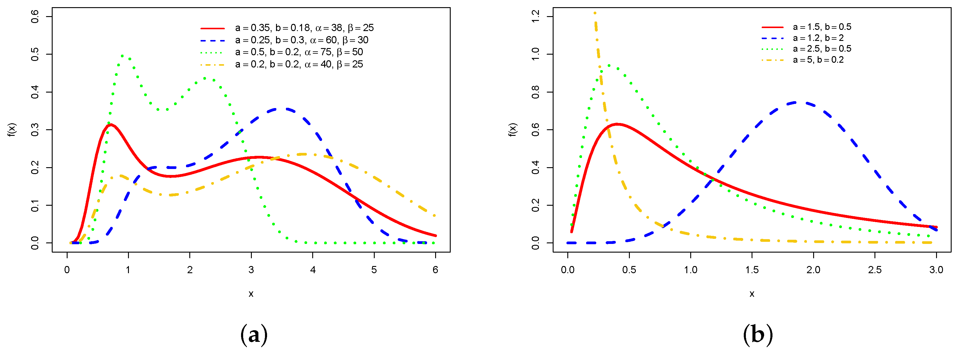
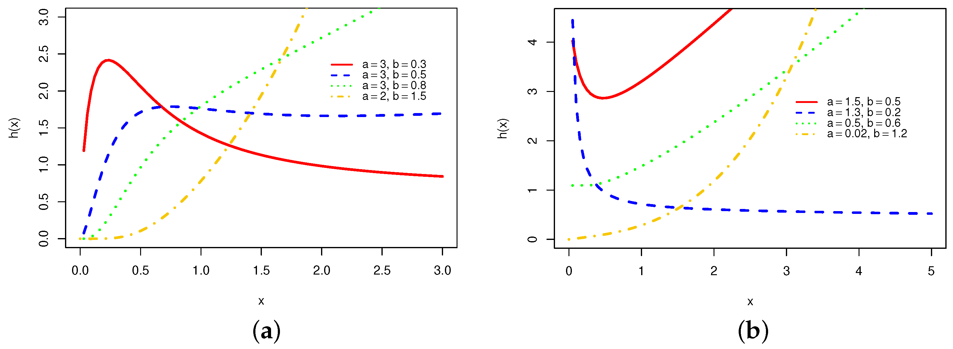
Henceforth, let $X\sim \mathrm{W}\mathrm{B}\mathrm{P}(a,b,\alpha ,\beta )$ have pdf (4). Figure 1 and Figure 2 report plots of the pdf and hrf of X, respectively. Figure 1a shows that the WBP distribution can model data with bimodality. The hrf in Figure 2 can have four main shapes.

The main motivation to introduce the WBP distribution is due to the wide use of the BP distribution and the fact that the current generalization provides better fits to complex real data.

3. Properties

3.1. Quantile Function

By inverting the W-G family cdf, the quantile function (qf) of X reduces to

$$\begin{array}{c}\hfill x=Q\left(u\right)=F^{-1}\left(u\right)=G^{-1}\left(\frac{{\left\{log\left[-a^{-1}(1-u)\right]\right\}}^{1/b}}{1+{\left\{log\left[-a^{-1}(1-u)\right]\right\}}^{1/b}}\right),\end{array}$$

(6)

$G^{-1}\left(u\right)$ follows by inverting (1)

$$\begin{array}{c}\hfill G^{-1}\left(u\right)==\frac{I_u^{-1}(\alpha ,\beta )}{1-I_u^{-1}(\alpha ,\beta )},\end{array}$$

where $I_u^{-1}(\alpha ,\beta )$ is the inverse incomplete beta function, which can be calculated from InverseBetaRegularized[u,a,b] (in MATHEMATICA) as

$$\begin{array}{cc}\hfill & I_u^{-1}(\alpha ,\beta )\approx u+\frac{\beta -1}{\alpha +1}{u}^2+\frac{(\beta -1)({\alpha }^2+3\beta \alpha -\alpha +5\beta -4)}{2{(\alpha +1)}^2(\alpha +2)}{u}^3+\cdots \hfill \end{array}$$

Plots of the Bowley skewness (B) [15] and Moors kurtosis (M) [16] of X based on octiles are given below.

For any fixed value of b, Figure 3a shows that the skewness decays when parameter a increases, showing more pronounced curvature for $b=3.5$. For $a=0.09$ and $a=0.1$, Figure 3b shows that the skewness starts constantly when b grows and then decays. For $a=0.2$ and $a=0.4$, it decreases almost instantly.

The behavior of the kurtosis is analogous as shown in Figure 4a,b. In Figure 4a, for any fixed value of b, the kurtosis decreases and then asymptotically approaches a constant when a increases. For $b=0.5$, this behavior is slower. In Figure 4b, the kurtosis decreases and becomes asymptotically constant when b grows. For $a=0.2$ and $a=0.4$, this behavior happens quickly.

3.2. Linear Representation

Proposition 1.

The WBP pdf (4) has the linear representation

$$\begin{array}{c}\hfill f\left(x\right)=\sum _{i,m=0}^{\infty }{B}_{i,m}g(x;{\alpha }_{i,m}^{\star },\beta ),\end{array}$$

(7)

where $B_{i,m}$’s are real numbers and ${\alpha }_{i,m}^{\star }\left(\alpha \right)=(i+1)\alpha +m$.

Proof of Proposition 1.

The density of X (except for typos) was determined by [1]

$$\begin{array}{c}\hfill f\left(x\right)=\sum _{j,k=0}^{\infty }{\omega }_{j,k}{h}_{(k+1)b+j}\left(x\right),\end{array}$$

(8)

where $h_p\left(x\right)=pg\left(x\right)G{\left(x\right)}^{p-1}$ (for $p>0$) and

$$\begin{array}{c}\hfill {\omega }_{j,k}={\omega }_{j,k}(a,b)=\frac{{(-1)}^{j+k}b{a}^{k+1}}{\left[\right(k+1)b+j]k!}\left(\genfrac{}{}{0pt}{}{-\left[\right(k+1)b+1]}{j}\right).\end{array}$$

In particular, for the BP baseline, we can expand

$$\begin{array}{c}\hfill I_z{(\alpha ,\beta )}^{(k+1)b+j-1}=\sum _{i=0}^{\infty }{s}_{i,j,k}{I}_z{(\alpha ,\beta )}^i,\end{array}$$

(9)

where $s_{i,j,k}=s_{i,j,k}\left(b\right)={\sum }_{l=i}^{\infty }{(-1)}^{i+l}\left(\genfrac{}{}{0pt}{}{(k+1)b+j-1}{l}\right)\left(\genfrac{}{}{0pt}{}{l}{i}\right)$, and then from (8)

$$\begin{array}{c}\hfill f\left(x\right)=\sum _{i=0}^{\infty }{A}_i{x}^{\alpha -1}{(1+x)}^{-\alpha -\beta }{I}_z{(\alpha ,\beta )}^i,\end{array}$$

(10)

where $A_i=A_i(a,b)=B{(\alpha ,\beta )}^{-1}{\sum }_{j,k=0}^{\infty }[(k+1)b+j]{\omega }_{j,k}{s}_{i,j,k}$.

The power series holds

$$\begin{array}{c}\hfill I_z(\alpha ,\beta )=\frac{z^{\alpha }}{B(\alpha ,\beta )}\sum _{m=0}^{\infty }{q}_m{z}^m,\left|z\right|<1,\end{array}$$

where $q_m=q_m(\alpha ,\beta )={(1-\beta )}_m/m!(\alpha +m)$ and ${\left(p\right)}_m=p(p-1)\dots (p-m+1)$ is the falling factorial. For a natural number $i\ge 1$, the Identity 0.314 in [17] gives

$${\left(\sum _{m=0}^{\infty }{q}_m{z}^m\right)}^i=\sum _{m=0}^{\infty }{e}_m^{\left(i\right)}{z}^m,$$

where $e_0^{\left(i\right)}=q_0^i$, and 

$$e_m^{\left(i\right)}=\frac{1}{m{q}_0}\sum _{l=1}^m[(i+1)l-m]q_l{e}_{m-l}^{\left(i\right)},i\ge 1,$$

Hence,

$$\begin{array}{c}\hfill I_z{(\alpha ,\beta )}^i=\frac{z^{i\alpha }}{B{(\alpha ,\beta )}^i}\sum _{m=0}^{\infty }{e}_m^{\left(i\right)}{z}^m,\left|z\right|<1.\end{array}$$

Letting $z=z\left(x\right)=x/(1+x)$,

$$\begin{array}{c}\hfill I_z{(\alpha ,\beta )}^i=\frac{1}{B{(\alpha ,\beta )}^i}\sum _{m=0}^{\infty }{e}_m^{\left(i\right)}\frac{x^{m+i\alpha }}{{(1+x)}^{m+i\alpha }},x>0.\end{array}$$

(11)

Furthermore, for $i=0$, let $e_0^{\left(0\right)}=1$, and $e_m^{\left(0\right)}=0$ for $m\ge 1$. Inserting (11) in Equation (10), and under the previous conditions, gives

$$\begin{array}{cc}\hfill f\left(x\right)& =\sum _{i,m=0}^{\infty }{B}_{i,m}g(x;{\alpha }_{i,m}^{\star },\beta ),\hfill \end{array}$$

(12)

where ${\alpha }_{i,m}^{\star }\left(\alpha \right)=(i+1)\alpha +m$, and 

$$B_{i,m}=B_{i,m}(a,b,\alpha ,\beta )=\frac{A_i(a,b)e_m^{\left(i\right)}B({\alpha }_{i,m}^{\star },\beta )}{B{(\alpha ,\beta )}^i},$$

which completes the proof.    ☐

Equation (12) confirms that the WBP density is a linear combination of BP densities, which is useful for finding properties of X. In fact, this representation is important since complete and incomplete moments, generating function, mean deviations, and reliability are well-known results for the BP distribution.

3.3. Moments

We obtain ${\mu }_s^{\prime }=E\left(X^s\right)$. For $s<\beta$, we can write from (12) and (3)

$${\mu }_s^{\prime }=\sum _{i,m=0}^{\infty }{B}_{i,m}\frac{B({\alpha }_{i,m}^{\star }+s,\beta -s)}{B({\alpha }_{i,m}^{\star },\beta )}·$$

(13)

The sth incomplete moment of X (for $s<b$) follows from (12) as

$$\begin{array}{cc}\hfill J_s\left(w\right)& ={\int }_0^w{x}^{s}f\left(x\right)\mathrm{d}x={\int }_0^w{x}^s\sum _{1,m=0}^{\infty }{B}_{i,m}g(x;{\alpha }_{i,m}^{\star },\beta )\mathrm{d}x\hfill \\ \hfill & =\sum _{i,m=0}^{\infty }{B}_{i,m}\frac{B({\alpha }_{m,l}^{\star }+s,\beta -s)}{B({\alpha }_{m,l}^{\star },\beta )}{I}_{w/(1+w)}({\alpha }_{i,m}^{\star }+s,\beta -s).\hfill \end{array}$$

The mean deviations and inequality measures are calculated from the first incomplete moment.

4. Estimation and Simulations

Let $x_1,\dots ,x_n$ be a sample from (4). The log-likelihood function for $\mathbf{\tau }={(a,b,\alpha ,\beta )}^{\top }$ is

$$\begin{array}{cc}\hfill l_n\left(\mathbf{\tau }\right)=& nlog\left[\frac{ab}{B(\alpha ,\beta )}\right]+(\alpha -1)\sum _{i=1}^{n}log{x}_i-(\alpha +\beta )\sum _{i=1}^{n}log(1+x_i)\hfill \\ \hfill & +(b-1)\sum _{i=1}^{n}log{I}_{z_i}(\alpha ,\beta )-(b+1)\sum _{i=1}^{n}log[1-I_{z_i}(\alpha ,\beta )]\hfill \\ \hfill & -a\sum _{i=1}^n{\left[\frac{I_{z_i}(\alpha ,\beta )}{1-I_{z_i}(\alpha ,\beta )}\right]}^b.\hfill \end{array}$$

(14)

The maximum likelihood estimates (MLEs) can be found via the Adequacymodel library [18] in R software by choosing a maximization method among those available.

Simulation Study

The simulation comprises the generation of samples from the WBP model from Equation (6) and maximizes (14) through the use of the BFGS algorithm in R for $n\in \{50,75,100\}$ from 10,000 replications under three scenarios: $a=0.75$, $b=1.5$, $\alpha =2.5$ and $\beta =2$ (Scenario 1); $a=0.75$, $b=1.2$, $\alpha =1$ and $\beta =1.5$ (Scenario 2); and $a=0.75$, $b=1.2$, $\alpha =2$ and $\beta =2.5$ (Scenario 3).

The findings in

Table 1. Simulation findings for the MLEs of the WBP distribution.

Scenario	n	Measures	Estimators
			$\widehat{\mathit{a}}$	$\widehat{\mathit{b}}$	$\widehat{\mathbf{\alpha }}$	$\widehat{\mathbf{\beta }}$
Scenario 1	50	Average	0.87959	1.22248	2.33968	2.05307
		Bias	0.12959	−0.27752	−0.16032	0.05307
		MSE	0.05690	0.10848	0.06048	0.02369
	75	Average	0.86856	1.22294	2.33987	2.04091
		Bias	0.11856	−0.27706	−0.16013	0.04091
		MSE	0.04698	0.10396	0.05023	0.01599
	100	Average	0.86195	1.22530	2.34140	2.03094
		Bias	0.11195	−0.27469	−0.15859	0.03094
		MSE	0.04223	0.10096	0.04198	0.01082
Scenario 2	50	Average	0.87959	0.99547	0.93431	1.54015
		Bias	0.12959	−0.20453	−0.06569	0.04015
		MSE	0.05690	0.05554	0.02394	0.03631
	75	Average	0.86856	0.99776	0.94906	1.53002
		Bias	0.11856	−0.20224	−0.05094	0.03002
		MSE	0.04698	0.04799	0.01850	0.03098
	100	Average	0.86195	1.00016	0.96222	1.52613
		Bias	0.11195	−0.19984	−0.03778	0.02613
		MSE	0.04223	0.04374	0.01424	0.02899
Scenario 3	50	Average	0.87959	0.99547	1.84264	2.57223
		Bias	0.12959	−0.20453	−0.15736	0.07223
		MSE	0.05690	0.05554	0.05855	0.05216
	75	Average	0.86856	0.99776	1.84443	2.56393
		Bias	0.11856	−0.20224	−0.15557	0.06393
		MSE	0.04698	0.04799	0.05382	0.04080
	100	Average	0.86195	1.00016	1.84516	2.55868
		Bias	0.11195	−0.19984	−0.15484	0.05868
		MSE	0.04223	0.04374	0.05201	0.03498

reveal (for all scenarios) that the biases and mean squared errors (MSEs) of the estimates decrease when n grows. Note that $\widehat{b}$ and $\widehat{\alpha }$ are underestimating b and $\alpha$ for all cases. All estimators improve when n increases.

5. WBP Regression Model

A WBP regression model is constructed for censored samples, quite common in areas such as econometrics, engineering, and clinical trials. Generally, for censored samples, it is common to consider the systematic component for the shape parameter $\alpha$. Thus, we consider the systematic component ${\alpha }_i=exp\left({\mathbf{v}}_i^{\top }\mathbf{\lambda }\right)$, where ${\mathbf{v}}_i^{\top }=(v_{i1},\cdots ,v_{ip})$ is the vector of covariates and $\mathbf{\lambda }={({\lambda }_1,\cdots ,{\lambda }_p)}^{\top }$ is the vector of unknown parameters. Let $\mathbf{v}={(v_1,\cdots ,v_p)}^{\top }$. Note that future research may be developed using more systematic components.

The survival function of $X_i|{\mathbf{v}}_i$ is

$$\begin{array}{c}\hfill S\left(x\right|{\mathbf{v}}_i)=exp\left\{-a{\left[\frac{I_z({\alpha }_i,\beta )}{1-I_z({\alpha }_i,\beta )}\right]}^b\right\}.\end{array}$$

(15)

Equation (15) defines the WPB regression model.

A special feature of survival data is the presence of censoring, which is the partial observation of the response. This refers to circumstances in which some subjects are free from the event of interest, for example, by being withdrawn early from the study or by the end of the experiment. Then, it is important to add this information to statistical modeling.

Let $(x_1,{\mathbf{v}}_1),\cdots ,(x_n,{\mathbf{v}}_n)$ be n independent observations, where $x_i$ denotes the observed lifetime or censoring time of the ith observation. Assume that the lifetimes and censoring times are independent, and their sets are F and C, respectively, i.e., the censoring is non-informative. The log-likelihood function for the vector of parameters $\mathbf{\tau }={(a,b,\beta ,{\mathbf{\lambda }}^{\top })}^{\top }$ from model (15) is

$$\begin{array}{ccc}\hfill l\left(\mathbf{\tau }\right)& =& rlog\left(ab\right)+\sum _{i\in F}({\alpha }_i-1)log\left(x_i\right)-\sum _{i\in F}({\alpha }_i+\beta )log(1+x_i)-\sum _{i\in F}log\left[B({\alpha }_i,\beta )\right]\hfill \\ & & +(b-1)\sum _{i\in F}log\left[I_{z_i}({\alpha }_i,\beta )\right]-(b+1)\sum _{i\in F}log[1-I_{z_i}({\alpha }_i,\beta )]\hfill \\ & & -a\sum _{i\in F}{\left[\frac{I_{z_i}({\alpha }_i,\beta )}{1-I_{z_i}({\alpha }_i,\beta )}\right]}^b-a\sum _{i\in C}{\left[\frac{I_{z_i}({\alpha }_i,\beta )}{1-I_{z_i}({\alpha }_i,\beta )}\right]}^b,\hfill \end{array}$$

(16)

where r is the number of failures. The estimate $\widehat{\mathbf{\tau }}$ is found by maximizing Equation (16).

5.1. Diagnostic and Residual Analysis

The assessment of robustness aspects of the estimates in regression models has been an important concern of various researchers in recent decades. The deletion measures examine the impact on the estimates after dropping individual observations, and they are the most employed technique to detect influential observations; see, for example, Ref. [19].

A global influence measure considered by [20] is a generalization of the Cook distance defined by a standardized norm ${\widehat{\mathbf{\theta }}}_{\left(i\right)}-\widehat{\mathbf{\theta }}$, namely

$$\begin{array}{c}\hfill G{D}_i\left(\mathbf{\theta }\right)={({\widehat{\mathbf{\theta }}}_{\left(i\right)}-\widehat{\mathbf{\theta }})}^{\top }\left[\ddot{\mathbf{L}}\left(\mathbf{\theta }\right)\right]({\widehat{\mathbf{\theta }}}_{\left(i\right)}-\widehat{\mathbf{\theta }}),\end{array}$$

(17)

where $-\ddot{\mathbf{L}}\left(\mathbf{\theta }\right)$ is the observed information matrix.

Another influence measure is the likelihood distance given by

$$\begin{array}{c}\hfill L{D}_i\left(\mathbf{\theta }\right)=2\left[l\left(\widehat{\mathbf{\theta }}\right)-l\left({\widehat{\mathbf{\theta }}}_{\left(i\right)}\right)\right],\end{array}$$

(18)

where $l(\widehat{\mathbf{\theta }})$ is the maximized log-likelihood function for the full sample and $l({\widehat{\mathbf{\theta }}}_{\left(i\right)})$ is the maximized log-likelihood function for the sample excluding the ith observation.

The quantile residuals (qrs) have the form

$$\begin{array}{c}\hfill q{r}_i={\mathsf{\Phi }}^{-1}\left(1-exp\left\{-\widehat{a}{\left[\frac{I_{z_i}({\widehat{\alpha }}_i,\widehat{\beta })}{1-I_{z_i}({\widehat{\alpha }}_i,\beta )}\right]}^{\widehat{b}}\right\}\right),\end{array}$$

(19)

where ${\mathsf{\Phi }}^{-1}(·)$ is the inverse of the standard normal cdf.

Various plots of these residuals can be adopted to assess the regression assumptions and detect influential observations.

5.2. Simulation Study

A simulation study examines the accuracy of the MLEs in the WBP regression model for $n=100$, 250, and 500 and censoring percentages 0%, 10%, and 30%. Here, 1000 replicates of each sample are generated using the inverse transformation method. The censoring times $c_1,\cdots ,c_n$ are obtained from a $\mathrm{Uniform}(0,\gamma )$, where $\gamma$ controls the censoring percentage. The systematic component for the parameter ${\alpha }_i$ (for $i=1,\dots ,n$) is

$$log\left({\alpha }_i\right)={\lambda }_0+{\lambda }_1{v}_{1i},$$

(20)

where ${\lambda }_0=1$, ${\lambda }_1=1.5$, $\sigma =0.3$, $a=1.1$, and $b=0.6$.

The simulation process follows as (for $i=1,\dots ,n$):

(i) Generate $v_{i1}\sim \mathrm{Uniform}(0,1)$, and calculate ${\alpha }_i$ from (20);

(ii) The generated lifetimes $x_i^{*}$ are determined from the WBP($a,b,{\alpha }_i,\beta$) model using Equation (6);

(iii) Generate $c_i\sim \mathrm{uniform}(0,\gamma )$ and obtain $x_i=\min (x_i^{*},c_i)$;

(iv) Set the censoring indicator: if $x_i^{*}<c_i$, then ${\delta }_i=1$; otherwise, ${\delta }_i=0$.

The values in

Table 2. Simulations from the WBP regression model.

			$\mathit{n}=100$			$\mathit{n}=250$			$\mathit{n}=500$
%	$\mathit{\tau }$	Averages	Biases	MSEs	Averages	Biases	MSEs	Averages	Biases	MSEs
$0\%$	${\lambda }_0$	1.3214	0.3214	0.6110	1.1415	0.1415	0.2501	1.0519	0.0519	0.1395
	${\lambda }_1$	1.5157	0.0157	0.3445	1.4956	−0.0044	0.1245	1.5054	0.0054	0.0584
	$\sigma$	0.4885	0.1885	0.1458	0.3724	0.0724	0.0383	0.3313	0.0313	0.0173
	a	1.1365	0.0365	0.6262	1.0916	−0.0084	0.2320	1.0843	−0.0157	0.1364
	b	0.5892	−0.0108	0.0593	0.6333	0.0333	0.0343	0.6564	0.0564	0.0251
$10\%$	${\lambda }_0$	1.3284	0.3284	0.6531	1.1450	0.1450	0.2611	1.0533	0.0533	0.1464
	${\lambda }_1$	1.5191	0.0191	0.3682	1.4960	−0.0040	0.1317	1.5055	0.0055	0.0604
	$\sigma$	0.5021	0.2021	0.1647	0.3755	0.0755	0.0414	0.3340	0.0340	0.0190
	a	1.1358	0.0358	0.6650	1.1093	0.0093	0.2959	1.0861	−0.0139	0.1462
	b	0.5884	−0.0116	0.0636	0.6341	0.0341	0.0371	0.6567	0.0567	0.0266
$30\%$	${\lambda }_0$	1.3866	0.3866	0.7464	1.1747	0.1747	0.2983	1.0727	0.0727	0.1707
	${\lambda }_1$	1.5168	0.0168	0.3956	1.5005	0.0005	0.1372	1.5088	0.0088	0.0660
	$\sigma$	0.5621	0.2621	0.2482	0.3955	0.0955	0.0546	0.3467	0.0467	0.0254
	a	1.1062	0.0062	0.5549	1.1055	0.0055	0.3272	1.0832	−0.0168	0.1625
	b	0.5737	−0.0263	0.0738	0.6238	0.0238	0.0400	0.6501	0.0501	0.0286

reveal that the average estimates converge to the true parameters, and the MSEs and biases decrease when n grows. Furthermore, the biases and MSEs of the estimates become larger when the censoring percentage increases. Hence, we conclude that the estimators are consistent.

6. Applications

First, the fits of the WBP, BP, Beta Beta Prime (BBP), and Kumaraswamy Beta Prime (KwBP) distributions are compared. The BBP and KwBP are special models of the McDonald inverted beta (McIB) [13].

For all fitted models, we calculate the MLEs and their standard errors (SEs). The well-known statistics (AIC, CAIC, BIC) defined by the initial letters are also calculated to compare the WBP distribution with its nested BP model. The Cramer–Von Mises ($W^{*}$), Anderson–Darling ($A^{*}$) and Kolmogorov–Smirnov (K-S) (and its p-value) statistics compare the WPB model with other distributions using the AdequacyModel [18], MASS and GenSA libraries of the R software. The maximization is performed using the SANN method.

6.1. Application 1: COVID-19 Data in the US

The first data set refers to 95 daily new deaths due to COVID-19 in the US (from 2 April 2021 to 31 July 2021) extracted from the link: https://www.worldometers.info/coronavirus/country/us/. This data set is used since the US is currently the country with the highest number of deaths from COVID-19. In the period, we find an average of 499.56 new deaths daily, and a standard deviation of 222.69, which can be explained by the evident variation in the number of daily deaths. In fact, the minimum number of daily deaths is 158 deaths, and the maximum is 985. In addition, we obtain skewness = 0.44 and kurtosis = 2.06.

Table 3. Findings for COVID-19 data in US.

Distribution	$\widehat{\mathit{a}}$	$\widehat{\mathit{b}}$	$\widehat{\mathit{\alpha }}$	$\widehat{\mathit{\beta }}$
WBP	1.2429	4.5036	33.4668	0.2694
	(0.3271)	(0.3768)	($1.5\times {10}^{-5}$)	(0.0115)
KwBP	25.7127	78.0954	8.8654	0.47724
	(0.0551)	(0.0266)	(0.0549)	(0.0056)
BBP	46.0854	32.1934	14.8327	0.2898
	(0.0087)	(0.0098)	(0.8696)	(0.0035)
BP	-	-	10.0000	0.2753
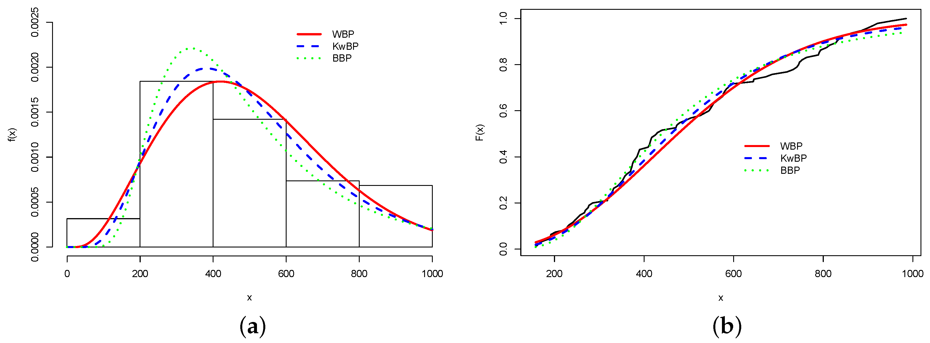
	-	-	(2.1758)	(0.0313)

reports the MLEs and their SEs (in parentheses). The statistics (and the p-values of K-S) are reported in

Table 4. Adequacy measures for COVID-19 data in US.

Distribution	${\mathit{W}}^{*}$	${\mathit{A}}^{*}$	K-S	p-Value	AIC	CAIC	BIC
WBP	0.1061	0.7499	0.2517	$\mathbf{1}.\mathbf{2}\times {\mathbf{10}}^{-\mathbf{5}}$	1350.97	1351.41	1361.19
KwBP	0.1104	0.8457	0.3425	$4.2\times {10}^{-10}$	1394.51	1394.96	1404.73
BBP	0.1142	0.8814	0.3504	$1.5\times {10}^{-10}$	1424.63	1425.07	1434.84
BP	0.1166	0.9023	0.4934	<$2.2\times {10}^{-16}$	1595.83	1595.96	1600.94

. The WBP distribution is better than the KwBP, BBP, and BP models.

The generalized likelihood ratio (GLR) test [21] assesses if there is any significant difference in the fits of the distributions. The WBP model outperforms the KwBP (GLR = 4.18) and BBP (GLR = 4.99) distributions for a significance level of 5%.

Figure 5a displays the histogram and the estimated WBP, KwBP, and BBP densities. Figure 5b reports the empirical and estimated cumulative distributions. The WBP distribution yields the best fit for a significance level of 5%.

6.2. Application 2: COVID-19 Data in Florianópolis, Brazil

According to the Votorantim Institute’s COVID-19 Municipal Vulnerability Index (MVI), Florianópolis is the least vulnerable capital to COVID-19 in Brazil [22]. In this context, the second application refers to 116 times (in days) of COVID-19 patients from the date of hospitalization until death in the city of Florianópolis registered from January to March, 2022 in the Ministry of Health platform at https://dados.gov.br/dataset/bd-srag-2021 (accessed on 26 May 2022). The average number of days from hospitalization to death is approximately 9.71 for patients in the analyzed period. The standard deviation is 7.67, which can be explained by the variation in these times. In fact, the minimum time from hospitalization to death is just only one day and the maximum 29 days. Furthermore, the skewness is 0.81 and the kurtosis 2.75.

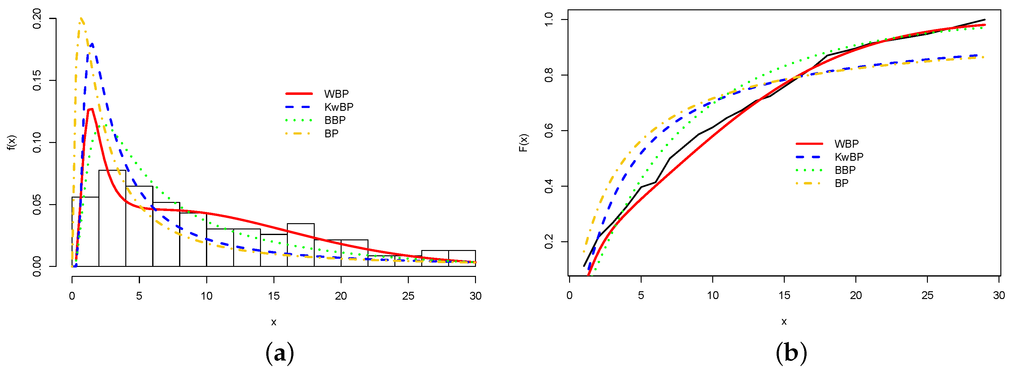
The MLEs, SEs, and the previous statistics (with the p-values of K-S) for the fitted distributions to these data are reported in

Table 5. Findings for COVID-19 data in Florianópolis.

Distribution	$\widehat{\mathit{a}}$	$\widehat{\mathit{b}}$	$\widehat{\mathit{\alpha }}$	$\widehat{\mathit{\beta }}$
WBP	0.3543	0.1876	38.2987	10.0908
	(0.0550)	(0.0161)	(0.3971)	(0.4519)
KwBP	2.2611	0.0648	10.3668	13.5489
	(0.0004)	(0.0060)	(0.0002)	(0.0001)
BBP	0.0619	38.7466	88.5759	0.5290
	(0.0058)	(0.0009)	(0.0006)	(0.0110)
BP	-	-	2.1732	0.7719
	-	-	(0.2970)	(0.0881)

and

Table 6. Adequacy measures for COVID-19 data in Florianópolis.

Distribution	${\mathit{W}}^{*}$	${\mathit{A}}^{*}$	K-S	p-Value	AIC	CAIC	BIC
WBP	0.4177	2.9113	0.2102	$\mathbf{7}.\mathbf{1}\times {\mathbf{10}}^{-\mathbf{5}}$	800.02	800.38	811.03
KwBP	0.5118	3.4879	0.3246	$4.9\times {10}^{-11}$	833.40	833.76	844.42
BBP	0.5653	3.8228	0.2874	$9.5\times {10}^{-9}$	824.16	824.53	835.18
BP	0.5025	3.4383	0.2409	$2.9\times {10}^{-6}$	827.23	827.34	832.74

. The numbers in the second table support that the WBP distribution is the best model.

The Vuong test [21] indicates that the new distribution is more adequate than the KwBP (GLR = 8.08) and BBP (GLR = 5.77) distributions for a 5% level of significance. A comparison of the WBP distribution with its BP sub-model gives LR = 31.21 (p-value = 1.668$\times {10}^{-7}$). Thus, the WBP distribution is the best one to describe the current data.

The histogram of the data and some estimated densities are reported in Figure 6a. Figure 6b displays the empirical and estimated cumulative distributions. They show that the WBP is the best model for these data.

6.3. Application 3: COVID-19 Data in Campinas, Brazil

Some regression models are fitted to 655 survival times of coronavirus patients hospitalized (on April 2021) in the city of Campinas (state of São Paulo) obtained from https://opendatasus.saude.gov.br/en/dataset/srag-2021-e-2022 (accessed on 1 September 2022). This city has the third largest municipal population in this State, around 1,213,792 people in 2020 according to the Brazilian Institute of Geography and Statistics (IBGE) [23], thus justifying its choice for the application. The censoring percentage (67.8%) refers to deaths from other causes or end of observation time. The survival time is the period of time (in days) from the first symptom to the death from COVID-19.

The covariates are (for $i=1,\dots ,655$):

• $x_i$: observed time (in days);
• $cen{s}_i$: censoring indicator (0 = censoring, 1 = observed lifetime);
• $v_{i1}$: age (in years);
• $v_{i2}$: Chronic cardiovascular pathology (1=yes, 0=no or not informed).

Other studies have analyzed the influence of covariates on the time to death from COVID-19. Ref. [24] analyzed coronavirus data in Curitiba, (Brazil) and verified the influence of the sex and age on the times (in days) elapsed from the date of hospitalization to the death. Ref. [25] investigated risk factors associated with these deaths in the Mexican population using survival analysis and concluded that the risk of death was higher for men, older individuals, chronic kidney disease patients, and people admitted to public health services.

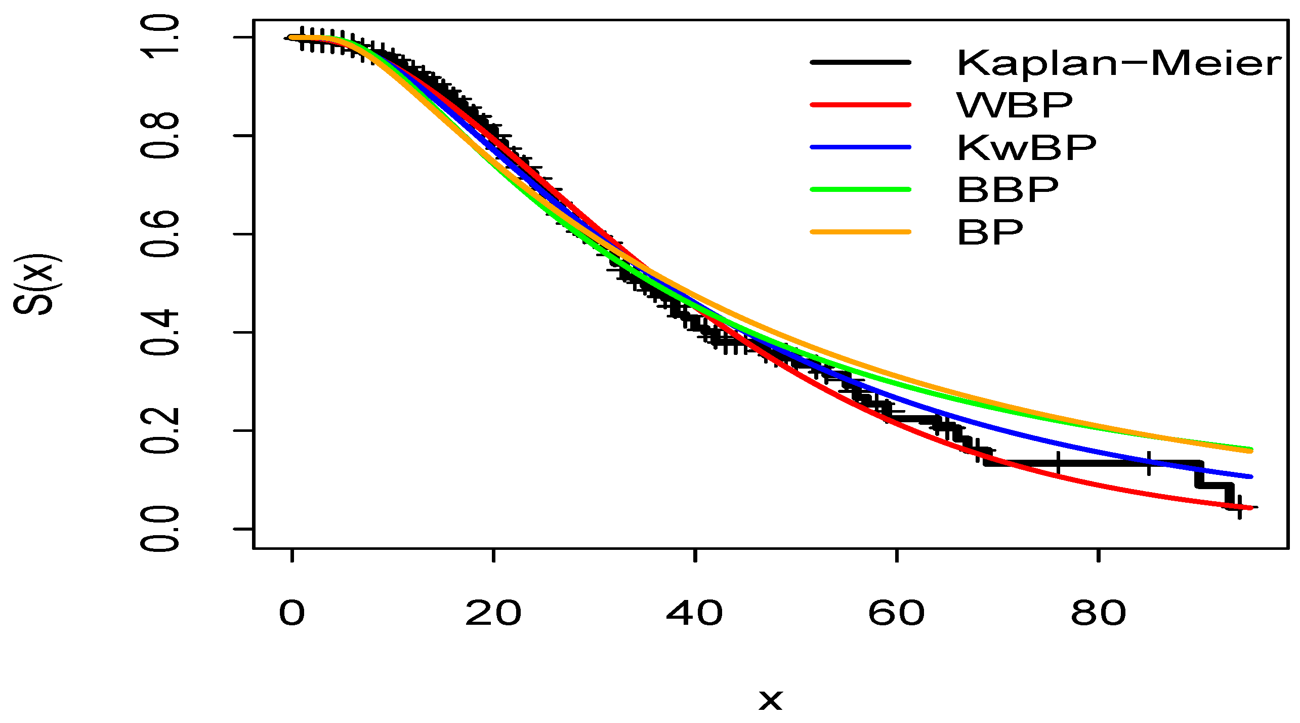
First, the analysis is done by modeling only the response variable by fitting the WBP, KwBP, BBP, and BP distributions. The results of these preliminary analyses are reported in Figure 7, where the WBP distribution is better than the others.

Next, we consider the following systematic components:

$${\mathcal{M}}_0:log\left({\alpha }_i\right)={\lambda }_0,$$

$${\mathcal{M}}_1:log\left({\alpha }_i\right)={\lambda }_0+{\lambda }_1{v}_{1i},$$

$${\mathcal{M}}_2:log\left({\alpha }_i\right)={\lambda }_0+{\lambda }_2{v}_{2i},$$

$${\mathcal{M}}_3:log\left({\alpha }_i\right)={\lambda }_0+{\lambda }_1{v}_{1i}+{\lambda }_2{v}_{2i}.$$

Table 7. Adequacy measures from regression models for COVID-19 data in Campinas.

Model		AIC	BIC	CAIC	Model		AIC	BIC	CAIC
${\mathcal{M}}_1$	WBP	2093.696	2111.635	2115.635	${\mathcal{M}}_3$	WBP	2071.653	2094.076	2099.076
	BBP	2160.907	2178.845	2182.845		BBP	2140.201	2162.624	2167.624
	KwBP	2111.858	2129.796	2133.796		KwBP	2090.371	2112.794	2117.794
	BP	2148.946	2157.915	2159.915		BP	2127.432	2140.885	2143.885
${\mathcal{M}}_1$	WBP	2046.338	2068.762	2073.762	${\mathcal{M}}_3$	WBP	2041.642	2068.550	2074.550
	BBP	2128.641	2151.064	2156.064		BBP	2122.585	2149.493	2155.493
	KwBP	2071.496	2093.919	2098.919		KwBP	2065.202	2092.110	2098.110
	BP	2115.254	2128.708	2131.708		BP	2109.588	2127.527	2131.527

gives the selection criteria values, and the WBP regression model has the lowest values for all systematic components. Note that this model with the structure ${\mathcal{M}}_3$ is superior to the other models.

The WBP, BBP, KwBP, and BP regression models with the structure ${\mathcal{M}}_3$ are evaluated using the quantile–quantile (QQ) and Worm plots of the qs in Figure 8 and Figure 9, respectively. The WBP regression model-${\mathcal{M}}_3$ is better than the others in agreement with the results in Table 7.

The findings in the final WBP regression model- ${\mathcal{M}}_3$ are given in

Table 8. Estimation results from the WBP regression model for COVID-19 data in Campinas.

	MLEs	SEs	p-Values
${\lambda }_0$	0.2154	0.0497	<0.001
${\lambda }_1$	−0.0099	0.0010	<0.001
${\lambda }_2$	−0.1257	0.0338	<0.001
$log\left(\beta \right)$	−1.5956	0.0066	<0.001
$log\left(a\right)$	−2.1310	0.0485	<0.001
$log\left(b\right)$	1.6418	0.0272	<0.001

, where two covariables are significant.

Figure 10 displays the index plots of the case deletion measures $G{D}_i\left(\mathbf{\theta }\right)$ and $L{D}_i\left(\mathbf{\theta }\right)$. From Figure 10a, the 323th, 409th, and 584th cases are possible influential observations referring to the following patients:

• 323th: A 42-year-old patient with failure time equal to one day who does not have cardiovascular disease;
• 409th: A 64-year-old patient with a failure time of one day who has cardiovascular disease;
• 584th: A 57-year-old patient with a failure time of one day who has cardiovascular disease.

Added Figure 10.

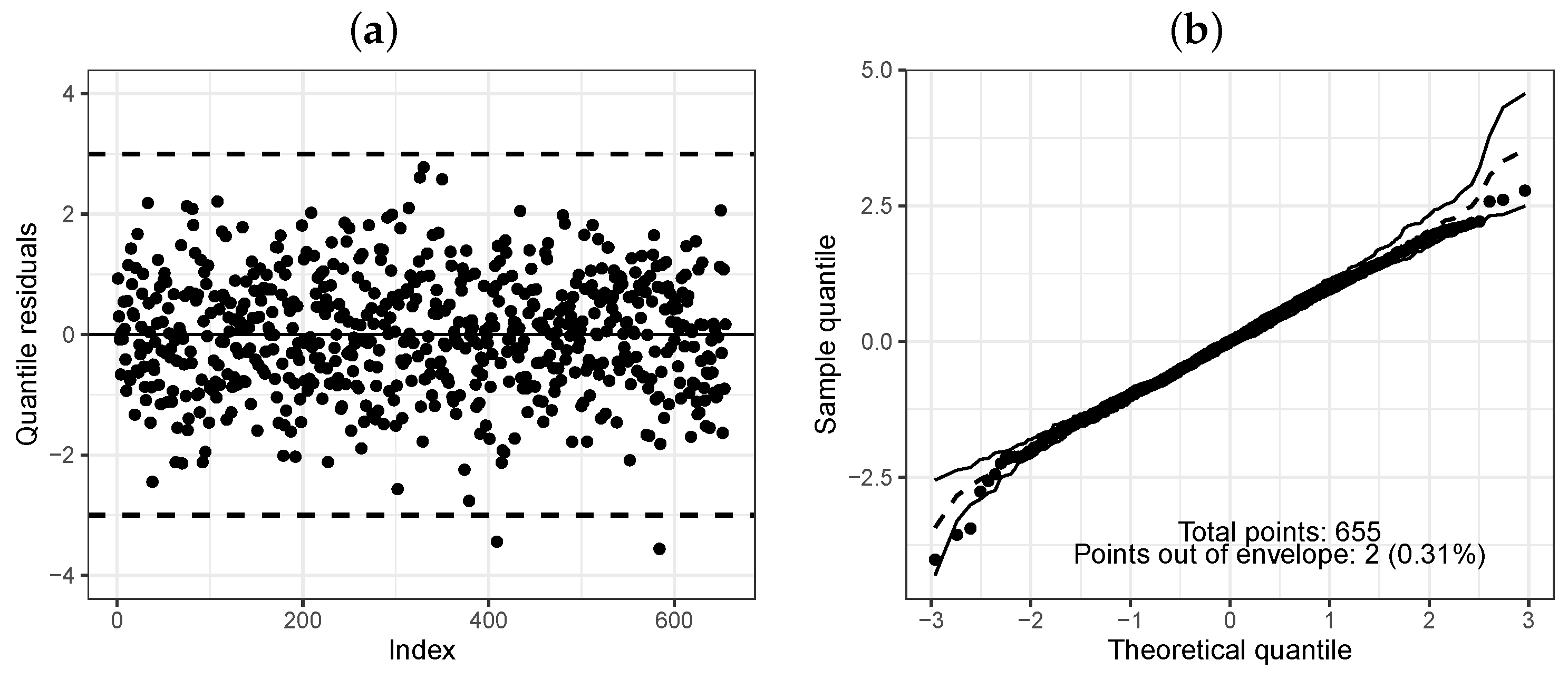
We examine the quality of fit of the WBP regression model—${\mathcal{M}}_3$. The qrs are randomly around zero as shown in Figure 11a. The QQ plot of these residuals with a simulated envelope [26] is displayed in Figure 11b. We can accept that there is evidence of a good fit of the WBP regression model.

Some interpretations of the final WBP regression model:

• The survival time tends to decrease when the patient gets older;
• There is a difference for the survival times between patients with chronic cardiovascular disease and those that do not present this condition.

7. Conclusions

We proposed a four-parameter Weibull beta prime (WBP) distribution. The estimation was conducted by the maximum likelihood method, and a simulation study showed the consistency of the estimators. We constructed a WBP regression model for censored data and proved the importance of the new models using three COVID-19 data sets. They were compared with some known competing models, and they were more suitable to fit all data sets. The regression model with censored data from COVID-19 patients showed that advanced age and cardiovascular disease are significant factors for the survival time. We concluded that the proposed models can be interesting alternatives for symmetric and asymmetric data, with bimodal shapes, censored or uncensored. Finally, future extensions of the article include, for example, other systematic components, thus defining heteroscedastic regression models based on the WBP distribution. In addition, generalizations of the new regression model for multivariate configurations and linear mixed effects models can be investigated.

References

1. Bourguignon, M.; Silva, R.B.; Cordeiro, G.M. The Weibull-G family of probability distributions. J. Data Sci. 2014, 12, 53–68. [Google Scholar] [CrossRef]
2. Eugene, N.; Lee, C.; Famoye, F. Beta-normal distribution and its applications. Commun. Stat.-Theory Methods 2002, 31, 497–512. [Google Scholar] [CrossRef]
3. Cordeiro, G.M.; de Castro, M. A new family of generalized distributions. J. Stat. Comput. Simul. 2011, 81, 883–898. [Google Scholar] [CrossRef]
4. Afify, A.Z.; Al-Mofleh, H.; Aljohani, H.M.; Cordeiro, G.M. The Marshall-Olkin-Weibull-H family: Estimation, simulations, and applications to COVID-19 data. J. King Saud Univ.-Sci. 2022, 34, 102115. [Google Scholar] [CrossRef]
5. El-Sherpieny, E.-S.A.; Almetwally, E.M.; Muhammed, H.Z. Bivariate Weibull-G Family Based on Copula Function: Properties, Bayesian and non-Bayesian Estimation and Applications. Stat. Optim. Inf. Comput. 2022, 10, 678–709. [Google Scholar] [CrossRef]
6. Almongy, H.M.; Almetwally, E.M.; Alharbi, R.; Alnagar, D.; Hafez, E.H.; Mohie El-Din, M.M. The Weibull Generalized Exponential Distribution with Censored Sample: Estimation and Application on Real Data. Complexity 2021, 2021, 6653534. [Google Scholar] [CrossRef]
7. McDonald, J.B.; Richards, D.O. Model selection: Some generalized distributions. Commun. Stat.-Theory Methods 1987, 16, 1049–1074. [Google Scholar] [CrossRef]
8. Bourguignon, M.; Santos-Neto, M.; de Castro, M. A new regression model for positive random variables with skewed and long tail. Metron 2021, 79, 33–55. [Google Scholar] [CrossRef]
9. McDonald, J.B.; Butler, R.J. Regression models for positive random variables. J. Econom. 1990, 43, 227–251. [Google Scholar] [CrossRef]
10. McDonald, J.B.; Xu, Y.J. A generalization of the beta distribution with applications. J. Econom. 1995, 66, 133–152. [Google Scholar] [CrossRef]
11. Leão, J.; Bourguignon, M.; Saulo, H.; Santos-Neto, M.; Calsavara, V. The Negative Binomial Beta Prime Regression Model with Cure Rate: Application with a Melanoma Dataset. J. Stat. Theory Pract. 2021, 15, 1–21. [Google Scholar] [CrossRef]
12. Medeiros, F.M.C.; Araújo, M.C.; Bourguignon, M. Improved Estimators in Beta Prime Regression Models. 2020, pp. 1–18. Available online: https://arxiv.org/pdf/2008.11750v1.pdf (accessed on 18 October 2021).
13. Cordeiro, G.M.; Lemonte, A.J. The McDonald inverted beta distribution. J. Frankl. Inst. 2012, 349, 1174–1197. [Google Scholar] [CrossRef]
14. Worldometer. COVID-19 CORONAVIRUS PANDEMIC. 2022. Available online: https://www.worldometers.info/coronavirus/ (accessed on 4 November 2022).
15. Kenney, J.F.; Keeping, E.S. Mathematics of Statistics. D. Nostrand Co. 1961, 1, 429. [Google Scholar]
16. Moors, J. A Quantile Alternative for Kurtosis. J. R. Stat. Soc. Ser. 1988, 37, 25–32. [Google Scholar] [CrossRef] [Green Version]
17. Gradshteyn, I.S.; Ryzhik, I.M. Table of Integrals, Series, and Products; Academic Press: Cambridge, MA, USA, 2000; Volume 1221. [Google Scholar]
18. Marinho, P.R.D.; Silva, R.B.; Bourguignon, M.; Cordeiro, G.M.; Nadarajah, S. AdequacyModel: An R package for probability distributions and general purpose optimization. PLoS ONE 2019, 14, e0221487. [Google Scholar] [CrossRef] [PubMed] [Green Version]
19. Cook, R.D.; Weisberg, S. Residuals and Influence in Regression; Chapman and Hall: New York, NY, USA, 1982. [Google Scholar]
20. Xie, F.C.; Wei, B.C. Diagnostics analysis in censored generalized Poisson regression model. J. Stat. Simul. 2007, 77, 695–708. [Google Scholar] [CrossRef]
21. Vuong, Q.H. Likelihood Ratio Tests for Model Selection and Non-Nested Hypotheses. Econom. J. Econom. Soc. 1989, 57, 307–333. [Google Scholar] [CrossRef] [Green Version]
22. Votorantim Institute. Browse the IVM Indicators. 2022. Available online: https://institutovotorantim.org.br/ivm/ (accessed on 4 November 2022).
23. Brazilian Institute of Geography and Statistics. Available online: ibge.gov.br (accessed on 7 November 2022).
24. Biazatti, E.C.; Cordeiro, G.M.; de Lima, M.C.S. The Dual-Dagum Family of Distributions: Properties, Regression and Applications to COVID-19 Data. Model Assist. Stat. Appl. 2022, 17, 199–210. [Google Scholar] [CrossRef]
25. Salinas-Escudero, G.; Carrillo-Vega, M.F.; Granados-García, V.; Martínez-Valverde, S.; Toledano-Toledano, F.; Garduño-Espinosa, J. A survival analysis of COVID-19 in the Mexican population. BMC Public Health 2020, 20, 1616. [Google Scholar]
26. Atkinson, A.C. Plots, Transformations, and Regression: An Introduction to Graphical Methods of Diagnostic Regression Analysis; Clarendon Press Oxford: Oxford, UK, 1985; Volume 282. [Google Scholar]
Figure 1. Density functions: (a) WBP( a , b , α , β ) and (b) WBP( a , b , 5 , 2.5 ).
Stats 05 00069 g001
Figure 2. Hazard rates: (a) WBP( a , b , 5.5 , 3 ) and (b) WBP( a , b , 2 , 4 ).
Stats 05 00069 g002
Figure 3. Plots of B for the WBP( a , b , 2.5 , 3 ) distribution: (a) for b fixed and (b) for a fixed.
Stats 05 00069 g003
Figure 4. Plots of M for the WBP( a , b , 2.5 , 3 ) distribution: (a) for b fixed and (b) for a fixed.
Stats 05 00069 g004
Figure 5. (a) Best estimated densities for COVID-19 data in US; (b) empirical and estimated cumulative distributions.
Stats 05 00069 g005
Figure 6. (a) Best estimated densities for COVID-19 data in Florianópolis; (b) empirical and corresponding estimated cumulative distributions.
Stats 05 00069 g006
Figure 7. Empirical and estimated survival functions for COVID-19 data in Campinas.
Stats 05 00069 g007
Figure 8. QQ plots of the qrs for COVID-19 data in Campinas from the regression models: (a) WBP; (b) BBP; (c) KwBP; (d) BP.
Stats 05 00069 g008
Figure 9. Worm plots of the qrs for COVID-19 data in Campinas from the regression models: (a) WBP; (b) BBP; (c) KwBP; (d) BP.
Stats 05 00069 g009
Figure 10. Index plots for: (a) G D i ( θ ) and (b) L D i ( θ ) .
Stats 05 00069 g010
Figure 11. Plots of the qrs for COVID-19 data in Campinas. (a) Index plot; (b) QQ plot with envelope.
Stats 05 00069 g011