1. Introduction
Due to the development and evolution of new IT tools in the new millennium, there is a vast amount and growing availability of heterogeneous, structured, and unstructured data, better known as “Big Data”. The term “Big Data”, already used in 1941 to quantify the so-called information explosion, is commonly used in every scientific research field and every business world sector. De Mauro et al. (2015) [
1] highlighted that Big Data is an “information resource”, since this entity is identifiable and does not depend on the field of application. They proposed the following formal definition: ≪Big Data represents the information assets characterized by high volume, velocity and variety to require specific technology and analytical methods for its transformation into value≫.
Due to the opportunities offered by using new sources and big data, the field of statistics has moved towards the modernization of methods and tools with a scientific revolution in which the datum becomes the raw material for change. In this cultural revolution, sampling plays a renewed but highly crucial role. Although sampling was born from the lack of data about the target population, in the era of “Big Data”, where a large production of and a quick availability of data are simple, some “classic” statistical techniques on “small” samples and statistical inference seem useless. However, big data hide many pitfalls including relevant and flattened relationships and information, heterogeneity, etc., and a large amount of data hides or highlights relationships when they exist or do not exist. The main problem is that big data are often not the result of a priori planned statistical surveys. Big data can be considered a non-probabilistic sample of a target population, and inference cannot be made [
2]. Non-sample biases usually affect non-probabilistic samples [
3]. These include coverage errors, which are the leading cause of the selection bias in big datasets. The results are probably valid for the sample units (internal validity) in these cases. Still, the results cannot be generalized (lack of external validity), and inference cannot be made.
From a practical point of view, there are many application areas where big data are currently being used with excellent prospects and potential without, however, considering that big datasets are non-probabilistic samples and are affected by selection bias, for instance, social media [
4], blogs, and web search keywords to trace desires, opinions, and sentiments; emails and phone contacts to trace social relationships; transaction records of our purchases to proxy for lifestyle and shopping patterns; records of our mobile phone calls and GPS trajectories to trace individuals’ movements; and so on [
5]. In education and training, data on student performance, learning mechanisms, and responses to different pedagogical strategies can help to better understand student knowledge and accurately assess student progress, mobility, and chain migrations [
6]. Moreover, in finance, business, marketing, and social marketing, so-called business data are gaining more relevance as more and more companies collect and produce huge amounts of data and contextual information. Further, big data are being considered to find solutions to manage and optimize the logistics and mobility of multimodal transportation networks in smart cities. A datacentric approach can also help to improve the efficiency and reliability of a transportation system. Moreover, georeferenced data fusion can help to obtain an efficient urban planning system that mixes public and private transport, offering people more flexible solutions. In energy resource optimization and environmental monitoring, the data related to electricity consumption and the analysis of load profiles are very important. Big datasets are analyzed entirely in these application domains without recourse to sampling or the considered populations. Recently, big datasets have been treated with sampling-related approaches, i.e., samples of the big datasets have been analyzed that could allow inferential analyses to be conducted. For example, Ahlawat et al. (2019) [
7] applied a cluster heads-based data-level sampling solution, which inherited the edge of k-means and fuzzy C-means clustering approaches. Abdullahi et al. (2019) [
8] used a mechanism to identify bandings in large “zero-one”
N-dimensional datasets, using a sampling technique. Liu and Zhang (2019) [
9] focused on the sampling techniques used for big data profiling. Hasanin et al. (2019) [
10] analyzed two case studies with six sampling approaches to investigate the effect of severe class imbalance on big data analytics.
From a statistical point of view, the methods to analyze big data that have been proposed in the scientific literature can be classified into three macrogroups: “divide and conquer” methods based on the original big dataset’s subdivision into small blocks that are manageable by the current computer processing unit; “fine to coarse” methods based on the rounding of parameters; and sampling methods based on a subsample of the original big dataset [
11]. These methods enable solving computational problems and optimizing the minimum necessary resources. Still, they do not affect the estimation procedure, and it, therefore, remains influenced by the assumptions and errors, especially the coverage errors, that caused the selection bias. The methods to correct the selection bias can be applied at the “unit-level” or “domain-level” [
12]. Based on information from auxiliary variables related to the variable of interest, they consider the selection bias and determine what comes from reliable sources. Unit-level methods include: “pseudo-design” methods based on the so-called “reweighting” of individual records (e.g., post-stratification [
13] and the Raking algorithm [
14]), methods based on a modeling approach (e.g., econometric selection models, “small area” estimation approaches, Bayesian or machine learning approaches, etc.); “data linking” approaches, in which the data are linked on an individual level with data of a target population frame or a sample of it to reweight or model the estimates. Domain-level methods include: “pseudo-design” methods based on the reweighting of the domain estimates (i.e., aggregated values for subpopulations or even for the entire population) and methods based on a modeling approach that assume the availability of an additional data source. These methods are applied to the whole big dataset and do not enjoy the computational advantages initially presented with the divide and conquer, fine to coarse, and sampling techniques.
One method that could possibly exploit the potential of big data and enable inference, considering also the non-sampling errors produced by the other V characteristics, is “inverse sampling”, first proposed by Hinkins et al. (1997) [
15] and deepened by Rao et al. [
16]. In his original formulation, Hinkins assumed working with a “bad” sample, affected by a non-probabilistic procedure to select the statistical units and by bias due to the use of data that were inaccurate and not necessarily structured (either by the sampling scheme or by the realization of it): he proposed a resampling scheme that led to the formation of a better subsample, referable to a simple random sample for the population (and not to the “poorly realized” sample). In this paper, we consider the so-called “novel inverse sampling”, based on the classical inverse sampling, proposed by Kim and Wang (2019) [
17], where the first bad-realized sample is, indeed, the big data. So, the computational aspects and the selection bias problem can be solved to obtain a probabilistic sample and valid inferential results. Many of the methods and applications for big data described above and in the literature, often do not consider the characteristics of velocity, variety, and veracity, focusing their attention only on the high volume to reduce the big data to a simple large dataset. Variety, veracity, and velocity influence, in fact, the availability of the dataset that moves too fast, presenting a different structure and architecture than the classical database and a low accuracy. So, if the volume affects the inference and sampling errors, the other aspects affect the non-sampling errors that, unfortunately, are neglected.
Although big data represent the information resources characterized by high volume, velocity, and variety that require specific technologies and analytical methods to transform into value, we will only consider volume in this paper. Velocity and variety will be assumed a priori as the big datasets’ characteristics. This paper explores the limits of inverse sampling for large datasets that are become smaller and smaller, assessing to what limit inverse sampling can be used. In addition, an analysis is conducted to assess the best sampling size of subsamples to extract, conducting evaluations in terms of the sampling rate. This provides empirical threshold values that allow us to determine the extent to which the results are valid.
The paper’s outline is as follows: after the introduction and background, in
Section 2, the methodology is introduced. In
Section 3, the simulation study and real case analysis are presented. Some final remarks follow.
2. Methodology
Kim and Wang (2019) [
17] proposed a method based on “inverse sampling” to solve computational aspects and the selection bias problem to obtain a probabilistic sample and valid inferential results. Inverse sampling, first proposed by Hinkins et al. (1997) [
15] and deepened by Rao et al. (2003) [
16], is a particular case of two-phase sampling also called double sampling [
18]. Inverse sampling was born as an approach to resample from a sample deriving from an already existing complex sampling plan (i.e., based on a complex extraction procedure) to obtain a data structure that was easier to analyze and as similar as possible to a simple random sample. It is graphically represented in
Figure 1.
For a further description of the algorithm, refer to [
15]. For more details on the definitions of extraction probabilities, inclusion probabilities, algorithms for the various existing sampling plans, the building of the estimator of the generic parameter
, the estimator’s properties, and the estimator’s variance, refer to Rao et al. (2003) [
16]. Kim and Wang (2019) [
17] proposed a method called “novel inverse sampling”, based on the classic inverse sampling, in which they treated the selection bias in big datasets with the approach of reweighting. Specifically, the first phase sample was the big dataset over which there was no control and was subject to selection bias. The second phase sample was a subsample of the big dataset.
Formally, Kim and Wang (2019) [
17] considered a finite population
, where
is the
i-th observation of the quantitative variable under study
Y, and
is the corresponding index with a known size equal to
N. There is a big dataset
, where
is considered a non-probabilistic sample from the finite population
. Let
denote the size of the big dataset. We also define an indicator variable
such that
if
, and
otherwise. We assume that
is observed if
, which leads us to consider the extraction process of the units
similar to a Bernoulli process. The parameter of interest is the population average
. The mechanism of
is crucial to determining the accuracy, measured by the total error influenced by the selection bias, of
as an estimator of
. Suppose the random mechanism for
is based on the Bernoulli sampling, where the indicator variables are independent and follow a Bernoulli distribution with probability
, through several steps. In that case, the total error can be expressed as ([
19]):
where
is the Pearson correlation coefficient between
and
Y.
Efron (1979) [
19] proved that only three factors determine the total error:
an increase in the quality of the data by reducing , where is the “data defect index”; this is the goal of all probabilistic sampling plans;
an increase in the quantity of the data by reducing , where represents the “dropout odds”: this is the advantage of big data; however, the impact of is much smaller than ;
a reduction in the difficulty of the estimating problem by reducing the degree of uncertainty , where represents the “degree of uncertainty”, with additional information.
Data quality is the most critical factor in accuracy and the most difficult to evaluate. For the sample average, it is captured by
because it accurately measures both the direction with the sign and the intensity of the selection bias caused by the
mechanism. The crucial result is that, for a fixed sampling rate
and problem difficulty
, the
for the sample average decreases at a rate of
, if
is controlled at
. Therefore, Efron (1979) [
19] ensured that all known probabilistic sampling plans were included in the definition, regardless of the
or the estimator choice.
In the building of the inverse sampling estimator, the first step is to control the selection bias through a reweighting approach characteristic of the pseudo-design methods that use reliable sources through auxiliary variables linked to the variable of interest. The second step is to select the second phase’s samples from the big dataset, with each unit’s selection probability proportional to the previously calculated weights. The final step is to carry out the usual estimation procedure on the extracted samples. The central assumption is that the selection process mechanism is conditionally independent of
Y given the auxiliary variable
X [
20]. We hypothesize that the selection mechanism is MAR (missing at random) in a missing data framework [
21]:
.
The generic inverse sampling estimator proposed is the simple average of the
g subsample estimators:
where:
The crucial point is the choice of the first-order conditional inclusion probabilities:
where the
are the “importance weights”, and
, with
. To estimate
, a calibration approach on the known population totals is used to modify the weights [
22], along with a reweighting method [
23]. The parametric probability density function for the auxiliary variable
x is approximated using the so-called “Kullback–Leibler Information” as the distance metric criterion [
24]. The solution is:
The solution of can be provided through iterative methods.
The variance of the inverse sampling estimator is ([
16]):
For the first term, we can apply the Horvitz–Thompson formula ([
25]):
where
is the second-order conditional inclusion probability.
Once the estimator and variance have been obtained, there is the possibility of testing the hypotheses parameters, constructing confidence intervals, etc. Starting from a non-probabilistic sample such as a big dataset, through inverse sampling, which allowed us to consider the effect of selection bias, we built some selection probabilities for the units. So, we obtained a probabilistic sample, an estimator, an estimator’s variance, and a theoretical basis for any inferential analysis. Therefore, our proposal worked by following these steps: through a simulation study and a real application, we explored the limitations of inverse sampling in cases where there were increasingly smaller big datasets, to empirically estimate the threshold values of the sampling size such that the inverse sampling continued to be a valid method. We evaluated the method in terms of bias, standard errors, and coverage of the estimators.
3. Numerical Study
This section shows the results of the studies conducted on simulated and real data to answer two questions, i.e.:
To do this, we assumed that veracity and variety were inherent characteristics of the big data. In the simulated case, we analyzed two different parameters (mean and proportion), while in the real case, we focused on proportion.
3.1. Simulated Case
A simulation study was carried out to evaluate our research question empirically. The idea was to assess how the bias changed as the size of the dataset on which we were working varied to determine whether the inverse sampling formalized for big datasets can be used in lower-dimensional contexts. The size of the population under study was constant (equal to 1,000,000); this was generated in the same way as the simulation presented by Kim and Wang (2019) [
17] (to maintain the comparability of results). Then,
where
, and the Gaussian noise was defined as
. From the population thus defined, several datasets
having the same amount of bias but different sizes
were extracted. The extraction of the biased dataset was also defined as in Kim and Wang (2019) [
17]. So, a source of selection bias was introduced into the big data extracted from the newly generated population. Then, we defined an inclusion indicator
, generated as
, where the
was defined as
The role of the
parameter is to introduce the bias that can be given by the variety, velocity, or veracity components typical of big data: the higher the value (considering the absolute value), the higher the bias. Finally, we defined
as the size of the extracted subsample from the datasets
. In
Table 1, we report the various values of
, and
used.
First of all, we were interested in the result concerning the parameter of the mean. In
Figure 2, the trend of the bias for different fixed values of
and the size
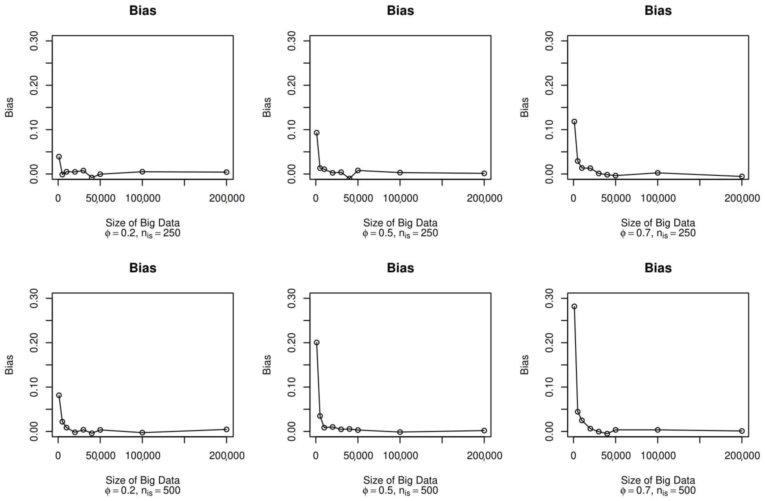
, for various sizes of the big data from which we extracted the subsamples, can be seen. In the six different scenarios, as the size of the big dataset increased, the estimation bias decreased. This result is entirely plausible, as a larger size of big data allows the inverse sampling to have a higher extraction capacity for observations that helps to constrain the selection bias of the big data. As the bias increased, the estimation bias increased, but this tended to even out when working with larger sizes of big data, i.e., over 50,000.
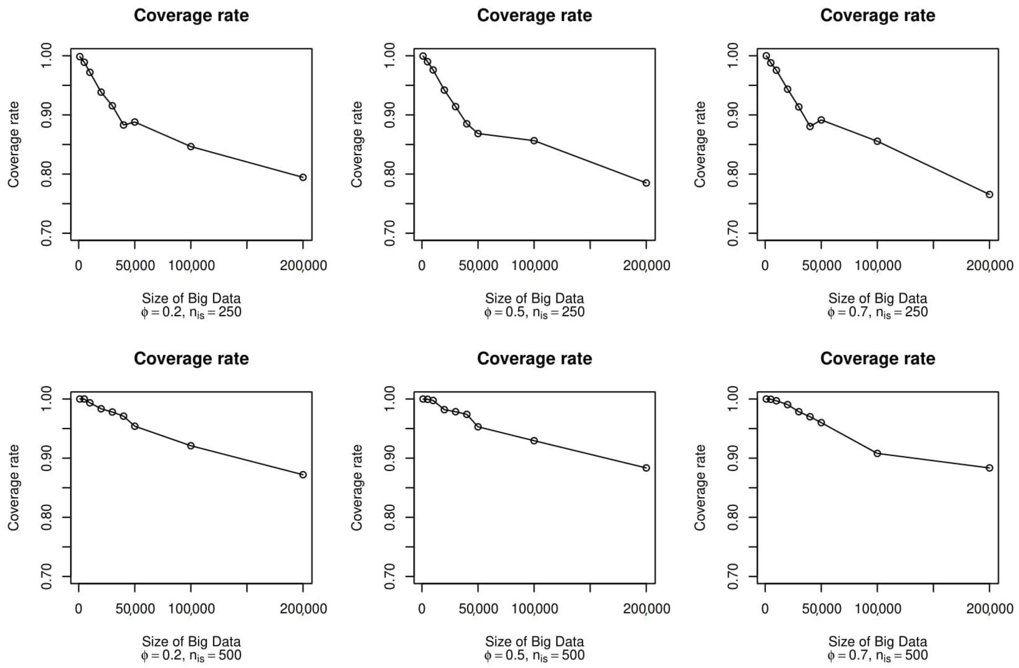
Figure 3 shows the coverage rate of the estimator. The six different scenarios are also shown for the coverage rate, varying the
. In the case of the subsamples with a size equal to 250, we observed almost identical coverage along with all the possible values of
. On the other hand, in the case of the subsamples with a size of 500, we observed that working with small sizes of big data led to a substantial reduction in coverage when working in contexts with medium or strong components of selection bias.
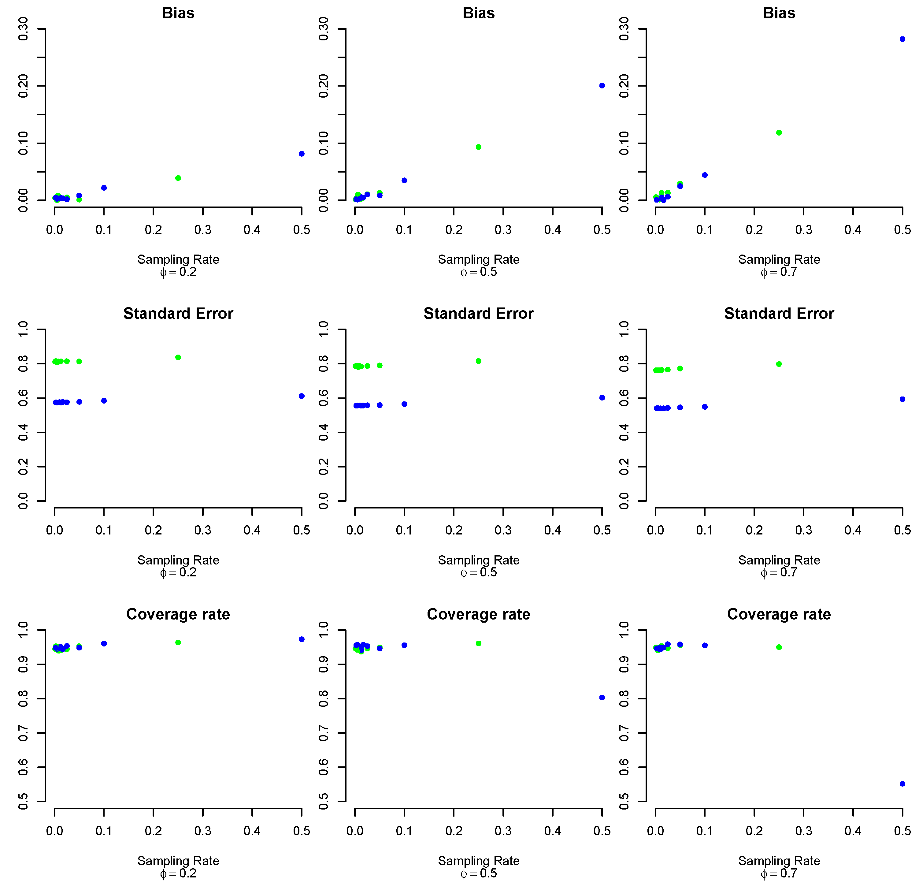
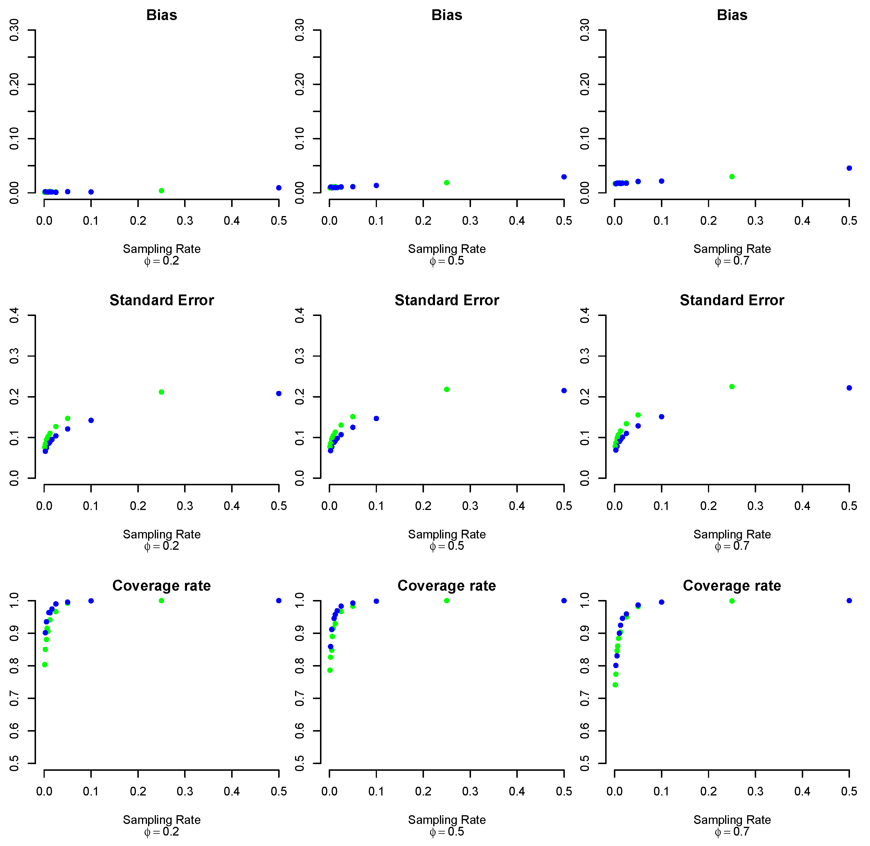
To determine the trend for the same quantities (along with the standard errors), we evaluated the graphs as a function of the sampling rate, defined as
.
Figure 4 shows the reference graphs. Beginning with the bias trend, as the sampling rate increased, the bias of the estimated parameter increased. This result can be attributed to the fact that, as we sampled (without repetition) more observations from the biased big data, more of the non-bias component was present in the subsamples. In fact, in scenarios where the bias component was smaller, the bias growth was significantly lower than in cases where
was larger.
For the standard errors, it can be seen that there were no substantial differences as the amount of bias or the sampling rate changed. In contrast, significant differences occurred according to the size of the extracted sample: the larger the size of the extracted subsample, the larger the standard error of the estimator.
It was possible to analyze the trend of the coverage rate: in the case where the bias was slight, the confidence intervals had optimal values regardless of the sampling rate; in the middle scenario, the coverage remained optimal, although, for a high sampling rate, considerably less coverage was observed. Finally, the coverage obtained with a high sampling rate dropped dramatically in the high-bias case. The declines in coverage can be attributed to the increase in bias observed in the same scenarios. This increase also did not involve the standard error, thus causing the construction of poor confidence intervals.
From these results, without knowing how high the bias component was, sampling up to 10% of the big data provided good results.
Table 2 reports the values shown on the graph and the standard errors of the estimates.
For the simulation study on the proportion estimator, the bias trend for the six settings as
varied is shown in
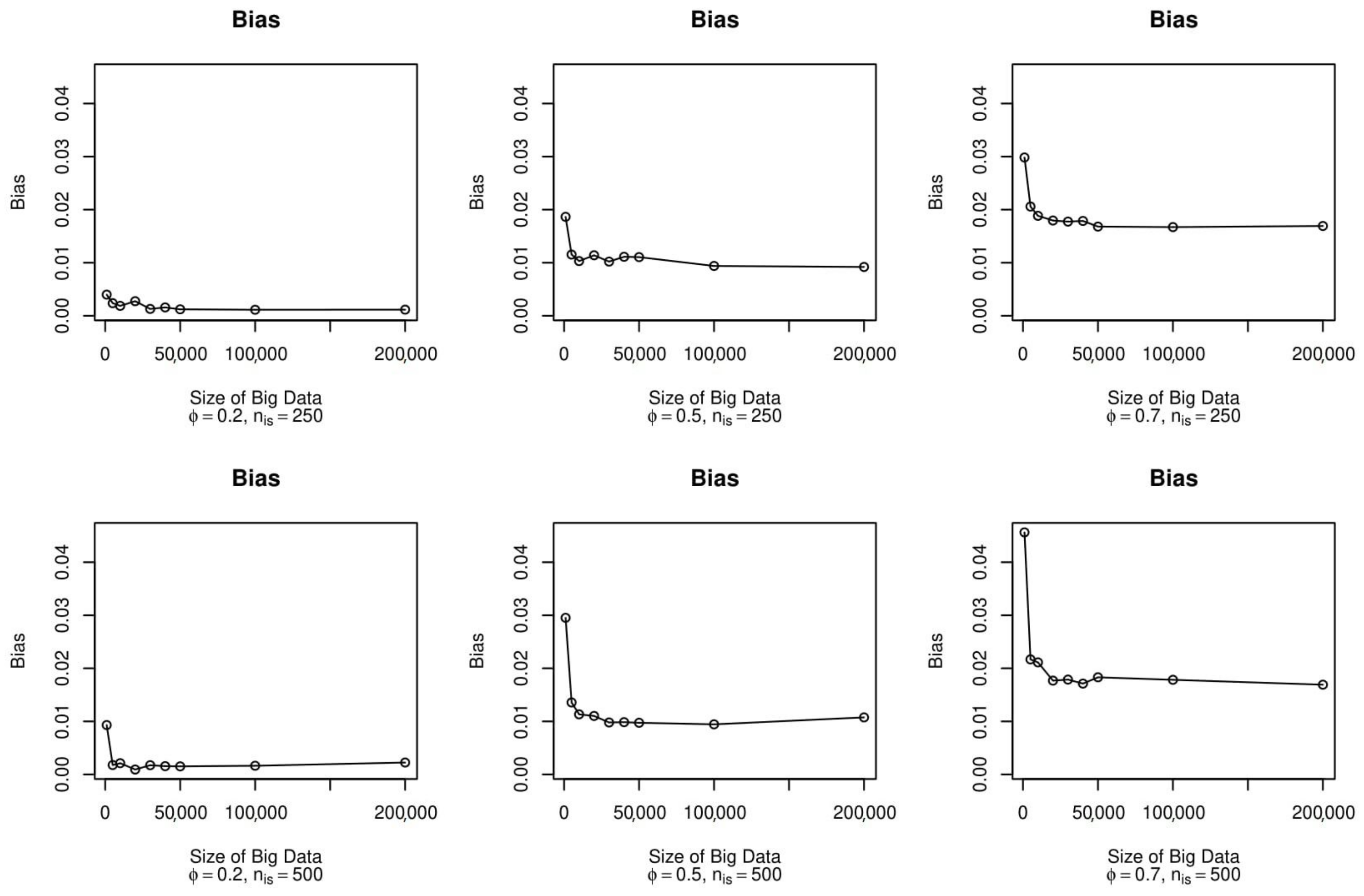
Figure 5. In the first case with subsamples equal to 250, the bias was almost always close to 0 in the case with lower bias, while the bias of the estimator increased (especially with very small sizes of big data) in the cases with higher bias. The scenarios did not change when extracting subsamples with a size equal to 500, where a higher bias was observed when the
was small.
Finally,
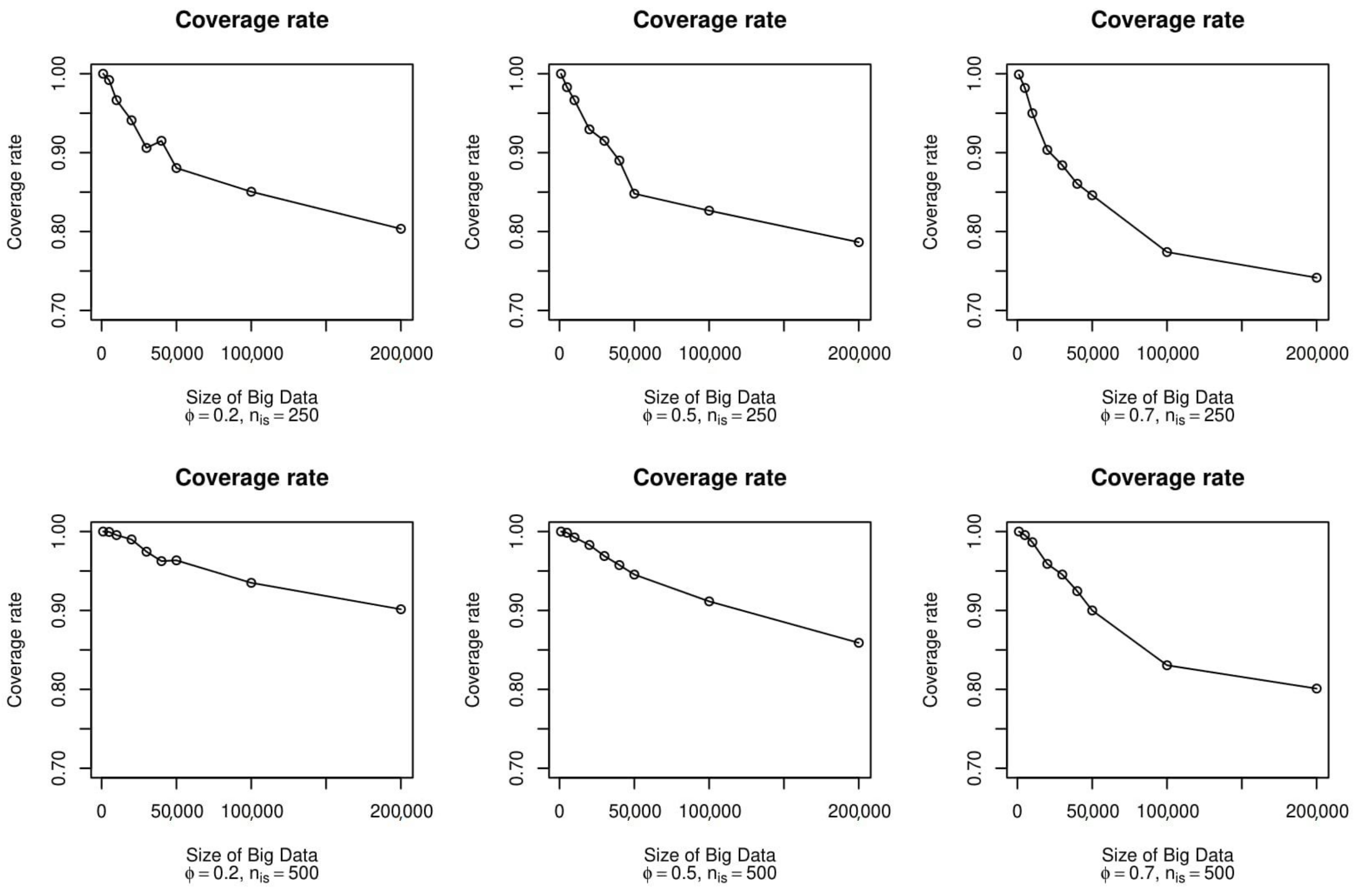
Figure 6 shows the behavior of the coverage rate of the estimator as the six scenarios changed. Here, there was a somewhat atypical trend of the coverage, as it decreased significantly when the size of the big data increased. This was probably due to the decrease in the standard errors of the estimate, while the bias did not become lower.
The evaluations made earlier for the bias remained the same. As the sampling rate increased, the bias increased accordingly for high-bias scenarios. On the other hand, different considerations needed to be made for the standard errors. Again, in this scenario, subsamples with larger numbers had a slightly larger standard error, but now the variability of the estimator increased as the sampling rate increased. This was reflected in the coverage rate of the confidence intervals, which had the opposite trend from those seen in
Figure 4: the coverage rate increased as the sampling rate increased, since the standard error also increased, so the intervals had larger widths.
Although the individual components of the estimator had different behaviors than in the case of the mean, the conclusions were still the same. The results for the bias and coverage seemed to have the best tradeoff with subsamples of about 10% of the big data.
Table 3 shows the values of the bias and coverage shown in the figure and with the standard deviation values.
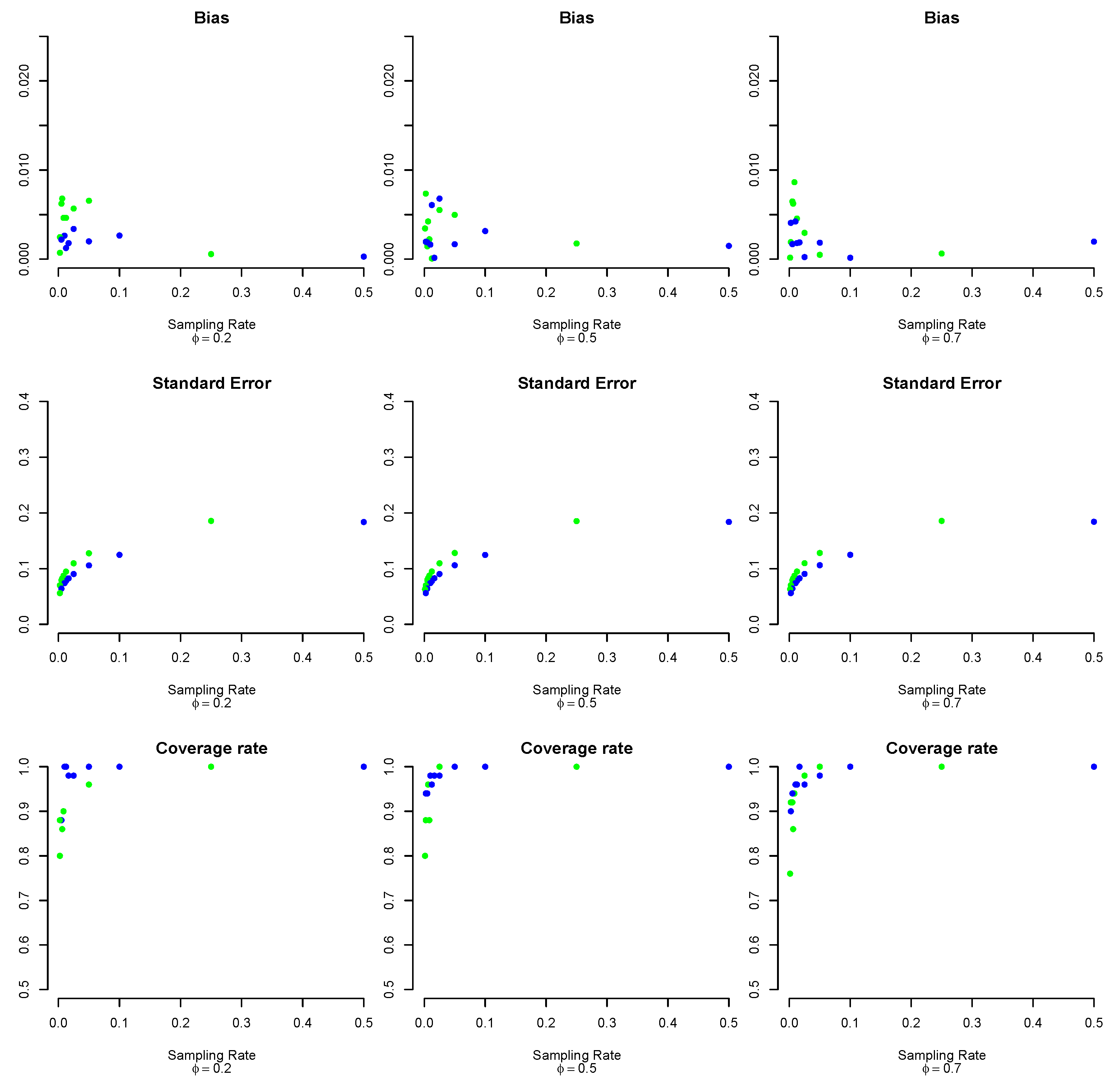
For the sampling rate, the results for the proportions are presented in
Figure 7.
3.2. Real Case
The dataset used for the real case contained the university careers of all students enrolled in Italian universities from 2017 to 2020. The statistical unit was a student enrolled in that period. We did not consider students enrolled in telematic universities because a parameter of interest was the proportion of enrolled “movers” (students whose residence region did not coincide with the region in which they chose to study). We also did not consider all new enrollments who had a year of birth before 1951. So, the dataset contained 1,149,504 observations. We considered this dataset the target population. A selection bias component was introduced to verify the method’s real ability to correct this source of error and the trend of the bias and coverage with the varied size of the biased big data. To introduce the bias component, we selected units as in Kim and Wang (2019) [
17]. For this reason, we were interested in finding a variable linked to the variable under study. Among the variables in the dataset, we decided to consider the “high school mark score”, because we saw that as the “high school mark score” increased, the proportion of movers showed a constant growth.
Since this dataset was population-based and, thus, by definition, free of selection bias, the bias component needed to be present to introduce some of the effects provided by velocity, variety, and veracity. To “create” this, the selection probability of the units was defined as the sigmoid function (inverse of the logit function):
where
is the auxiliary variable for the
i-th unit, and 67 is the first quartile of the “high school mark score”. We tried the method using the same setting described in
Table 1.
Figure 8 and
Figure 9 show the trends of the bias and coverage given the big datasets’ sizes and other scenarios considered. Considering the case with subsamples of size 250, the bias was remarkably reduced for the big data with a medium and high selection bias with respect to the simulated case, with the distance from the true value of the parameter close to 0. The coverage trend was almost equal to that of the simulated case, with a substantial decrease as the size of the big data increased.
Figure 10 shows the bias trend, standard error, and coverage, according to the sampling rate and amount of bias. The bias was slight in all the considered scenarios, and it tended to decrease as the sampling rate increased. The evaluations of the standard error were almost identical to those made in the simulations for the proportion estimator: it increased as the sampling rate increased, just as the standard error was greater when the size of the subsamples was 500. Finally, for the interval coverage rates, the conclusions were also the same as for the simulation results: the coverage reached satisfactory values for sampling rates above 5% (see
Table 4).
4. Conclusions
Sampling plays a crucial role in the new era of big data. Inverse sampling exploits big data’s potential and allows for inference. This paper investigated the limitations of inverse sampling for big data, analyzing when big data became too small in volume for inverse sampling and examining how much the method was affected by the sampling size of the subsamples. We then provided optimal threshold values to use. Two studies were conducted on simulated and real data, in which a selection bias component introduced the effects of velocity, variety and veracity.
In the simulation study, we proved (in an empirical way) that the method worked well even with a small dataset (with a size greater than or equal to ), and that the most important thing was to consider a reasonable sampling rate for the big data. There were some problems concerning the proportion parameter when the sampling rate was very small (under 5%). In the real case, we confirmed the results of the simulated case, where the coverage rate of the estimates increased according to the increase in the sampling rate.
Based on these results, inverse sampling is an excellent method for correcting selection bias (and all the problems that follow) and not just when working with big data having a very high volume. Even on smaller datasets affected by selection bias, the method proposed by Kim and Wang (2019) [
17] was successful. Therefore, this resampling technique may be extended to more scenarios not directly linked to the big data framework.
It may be of interest to carry out sensitivity analyses for future developments. The main assumption was about the MAR selection process. If this assumption is unlikely, one solution would be to evaluate different estimation scenarios and determine how consistent they are in terms of results. Another sensitivity analysis could be conducted by evaluating changes in terms of estimation by eliminating the most “influential” observations (in such a context, an influential observation is defined as an observation with an extreme importance weight associated with it, a value far removed from the other values of the importance weights).

