Article

Importance of Weather Conditions in a Flight Corridor

1
Chair of Econometrics and Statistics esp. Transportation, Dresden University of Technology, 01187 Dresden, Germany
2
Chair of Air Transport Technology and Logistics, Institute of Logistics and Aviation, Dresden University of Technology, 01062 Dresden, Germany
*
Author to whom correspondence should be addressed.
Stats 2022, 5(1), 312-338; https://doi.org/10.3390/stats5010018
Submission received: 13 February 2022 / Revised: 4 March 2022 / Accepted: 6 March 2022 / Published: 9 March 2022
(This article belongs to the Section Data Science)

Abstract

:
Current research initiatives, such as the Single European Sky Air Traffic Management Research Program, call for an air traffic system with improved safety and efficiency records and environmental compatibility. The resulting multi-criteria system optimization and individual flight trajectories require, in particular, reliable three-dimensional meteorological information. The Global (Weather) Forecast System only provides data at a resolution of around 100 km. We postulate a reliable interpolation at high resolution to compute these trajectories accurately and in due time to comply with operational requirements. We investigate different interpolation methods for aerodynamic crucial weather variables such as temperature, wind speed, and wind direction. These methods, including Ordinary Kriging, the radial basis function method, neural networks, and decision trees, are compared concerning cross-validation interpolation errors. We show that using the interpolated data in a flight performance model emphasizes the effect of weather data accuracy on trajectory optimization. Considering a trajectory from Prague to Tunis, a Monte Carlo simulation is applied to examine the effect of errors on input (GFS data) and output (i.e., Ordinary Kriging) on the optimized trajectory.

1. Introduction

With the implementation of Free Route Airspaces in Europe, wherein aircraft are requested to fly along four-dimensionally (longitude, latitude, altitude, and time) optimized trajectories, aircraft trajectory optimization gains more and more importance. One of the simplest aircraft motion models still induces six nonlinear first-order differential equations of motion. It follows that acceleration forces should be considered for each discrete time step. Besides aircraft performance parameters, the atmospheric state (specifically wind speed, wind direction, and temperature) has a significant impact on the integration of the equations of motion. Impulsive changes in weather data might lead to unrealistic fluctuations in acceleration forces between two consecutive time steps.
The aircraft performance model SOPHIA (Sophisticated Aircraft Performance Model) integrates the equations of motion every second and computes the actual speeds and covered distances. SOPHIA is largely based on pure physical laws, takes into account all acceleration forces, and uses the methodology from [1]. Coefficients that cannot be estimated without aircraft-specific aerodynamic properties (i.e., the drag polar and the maximum available thrust as a function of altitude and speed) are obtained from the open-source flight performance model OpenAP [2]. When optimizing the trajectory, target functions for speed and altitude are calculated by SOPHIA. In each time step, SOPHIA compares the actual speed and altitude with the target speed and target altitude and controls the lift coefficient in order to reach the target values in the next time step. Impulsive changes in the weather data between two consecutive time steps hamper the controller from reaching these target values. Furthermore, based on physic laws, atmospheric state parameters follow smooth functions. The gas-phase atmosphere is a fluid medium. Due to high kinetic energy and large distances, the molecules have enough time and space to move freely and quickly, which means that no large gradients can arise.
From the discussion above, it follows that functions describing weather data should be differentiable. This feature is not given by a linear interpolation, which results in a function consisting of several significant turning points, where its first-order derivative is not continuous. The necessity to apply a more sophisticated interpolation method to weather data follows, providing continuous and smooth functions, which are functions with continuous derivatives. In this study, we applied Kriging [3] to atmospheric state variables and validated the effect of smooth weather functions on the aircraft performance model SOPHIA. The Kernel method, including Kriging and Radial Basis Function (RBF) methods, can provide continuous and smooth functions, as noted by [4,5]. Further statistical interpolation methods, such as neural networks and decision trees, are also included for comparison, even though they might not lead to smooth results.
Meteorological data are provided by the Global Forecast System (GFS) (https://www.ncei.noaa.gov/products/weather-climate-models/global-forecast (accessed on 31 August 2020)), which combines data from various sources and produces forecasts of meteorological parameters such as temperature, wind speed, and wind direction [6]. GFS data are produced by the National Centers for Environmental Prediction (NCEP), a branch of the National Oceanic and Atmospheric Administration (NOAA). Each hour, NCEP obtains input data from the Global Data Assimilation System, which updates weather data from aircraft, weather stations, radars, and satellites and then predicts the weather conditions for a given point in time and space [7]. Unfortunately, the resulting data from GFS are too sparse for controlled trajectory optimization, and underlying models are too complex to be implemented for finer interpolation. Since 2018, the GFS has covered the entire globe with a base horizontal resolution of 1 degree (100 km) between grid points. Significant differences in weather data between 100 km are natural. Assuming usual aircraft cruising speeds of 200 m per second and discrete-time steps of 200 m, the flight performance model SOPHIA calculates at an approximate resolution of 200 m. Hence, SOPHIA interpolates approximately 500 times between two neighboured GFS data points. From this, it follows that a smooth function between two neighboured weather data points will result in a more realistic weather model. Operational forecasters use this GFS output to predict the atmospheric state up to 16 days in the future. If actual weather data are considered in trajectory optimization, simple linear interpolation between temporal-spatial points delivered by GFS is applied in [8,9,10]. Ref. [11] applies fourth-degree polynomials to fit wind data from NOAA. Kriging is often considered a benchmark for interpolation and has been applied in various human activity fields, for example, modelling surface-level wind speed [12], soil organic matter content [13], and air pollution [14]. Besides linear interpolation and Kriging, other regression models such as the decision trees and neural networks can be extended to perform interpolation tasks. We also considered the RBF methods. There already exist some comparisons and applications, but typically with a different objective. For example, ref. [15] compares the accuracy of Kriging and feedforward neural networks in predicting total dissolved gas in a dam’s reservoir. Ref. [16] uses neural networks to predict surface daily minimum temperature. Decision tree methods as random forest are applied by [17,18] to predict seabed sand content. This work applies and compares the accuracy of the following four methods to GFS weather data: linear interpolation, the RBF method, Kriging, feedforward neural networks, and decision tree methods. Therewith, we contribute by finding a more accurate interpolation in three-dimensional space, with temporal dimension being left to future research, for guaranteeing smooth weather data function for trajectory optimization. Moreover, we investigate the effect of the errors from the interpolation methods and GFS data on the optimal trajectory. Findings from our paper are unique and vital for the aircraft operators for relying on the interpolated weather data.
This paper is organized as follows. The first section describes weather variables in three spatial dimensions. Interpolation methods are introduced successively, along with parameter fitting, in Section 3. In the next section, these methods are compared based on accuracy regarding cross-validation. Finally, we take a trajectory from Prague to Tunis as an application and examine how the errors in GFS data and the interpolation method can impact the simulated trajectories.

2. Data

2.1. Data Sources

There are various weather data sources, but, unfortunately, most of them are not suitable for our study. Data from weather stations or weather services such as weather.com (accessed on 16 November 2020) or wetter.de (accessed on 16 November 2020) do not provide any information on the vertical dimension necessary for trajectory optimization. Well-known automatic dependent surveillance-broadcast (ADS-B) data collected along flights usually lack temperature, air pressure, wind speed, and wind direction information. These weather variables are often extracted from ADS-B data, as in [19,20], for further interpolation. In this work, we consider two important resources of weather data: GFS and weather balloon stations (https://www.ncei.noaa.gov/products/weather-balloon/integrated-global-radiosonde-archive (accessed on 18 December 2018)), also from NOAA.
Weather information about the troposphere is routinely collected with weather balloons released globally. In general, we prefer GFS data to weather balloon data as an input for trajectory optimization, due to the regular grid and higher resolution. A comparison of weather balloon stations and the GFS data grid can be found in Figure 1. In future research, we aim at fusing two sources for even more reliable data, but we concentrate on GFS data in the largest part of the current work. Later, in Section 4, we use balloon data to compare and evaluate interpolation results with GFS input.

2.2. Data Description

Two types of variables are used in GFS data, namely coordinate variables and weather variables. Coordinate variables mark the locations, including longitude (°), latitude (°), and altitude (°). The time domain is left for future research, and we believe that, as in the current examples, changes over time are not that great for a few-hour flight. Altitude is reported as geopotential altitude (m) and calculated from the gravity acceleration ( m · s 2 ). Weather variables include temperature (K), wind (m/s), relative humidity (%), and air pressure (hPa) for every coordinate variable set. We consider these variables because they are input variables for SOPHIA and included in GFS data, and it is a known fact that temperature and wind are crucial for trajectory optimization. The ground speed (m/s), i.e., the speed of an aircraft relative to the ground, can be calculated [21] with (m/s); V T is the true airspeed (m/s) relative to the still air; Z Wind and Z Temp are the wind vector and temperature (K); Mach denotes the Mach number, the vehicle airspeed relative to the speed of sound at current atmosphere condition; and k and R are constant for heat capacity ratio and gas constant, respectively. From this equation, we can see the importance of temperature and wind on the key parameters describing the status of an aircraft. The relative humidity is included in calculating contrail, see [8].
V G = V T + Z Wind , and V T = Mach k R Z Temp ,
Following notations in [22], let s = { s i } , with s i R d , i 1 , , n denote a series of n locations in a d-dimensional space. In our setup, d = 3 and the dimensional vector s i = ( s i , 1 , s i , 2 , s i , 3 ) corresponding to the longitude (°), latitude (°), and geopotential altitude (m). Let Z ( s ) = { Z ( s 1 ) , Z ( s 2 ) , , Z ( s n ) } be the sequence of random variables connected to the location s. For instance, Z ( s i ) can be temperature (K), wind (m/s), relative humidity (%), or air pressure (hPa) at location s i . Realizations of Z ( s ) are denoted by z ( s ) = { z ( s 1 ) , z ( s 2 ) , , z ( s n ) } .
As mentioned above, GFS offers structured data over a grid of longitudinal, latitudinal, and vertical points. Figure 2 is a three-dimensional snapshot of temperature data of this grid, at 1 degree or 100 km, by longitude and latitude. As for the altitude, the data are provided with the same pressure. These altitudes are still provided as geopotential altitudes, not “pressure altitudes” generated from pressure using exponential Formula (2), to be discussed at the end of this section. We generally operate below the troposphere, ranging from 0 to 11,000 m in geopotential altitude following the international standard atmosphere (ISA) [23]. The data are denser near the Earth’s surface with 200 m altitude resolution and sparser to around 2000 m at higher altitudes.
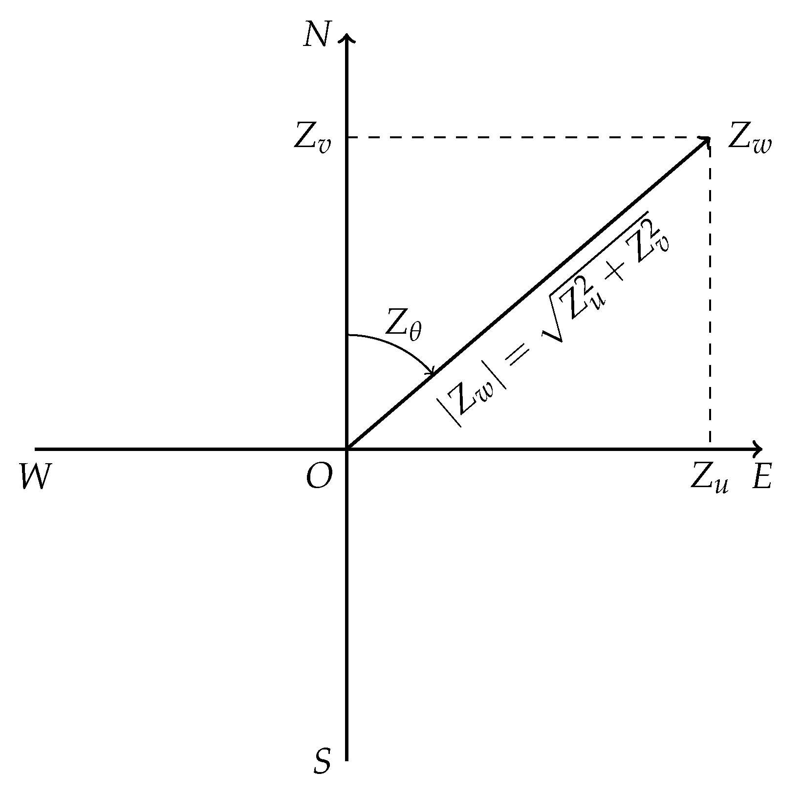
The wind is different from the other variables due to being a vector represented in a georeferenced coordinate system. A wind vector can be decomposed into two orthogonal components (see Figure 3); the U-wind (m/s) is the component from the west to the east, and the V-wind (m/s) is the component from the south to the north. Besides the two orthogonal components, wind vectors can also be denoted as wind speed (m/s) and direction (°). Wind speed is the length of this vector | Z w | = ( Z u 2 + Z v 2 ) 1 / 2 . Wind direction (°), Z θ in Figure 3, is the direction towards which the wind is blowing and measured by the angle from the true (geographic) north. GFS provides wind in U and V components, and we derive wind speed and direction.
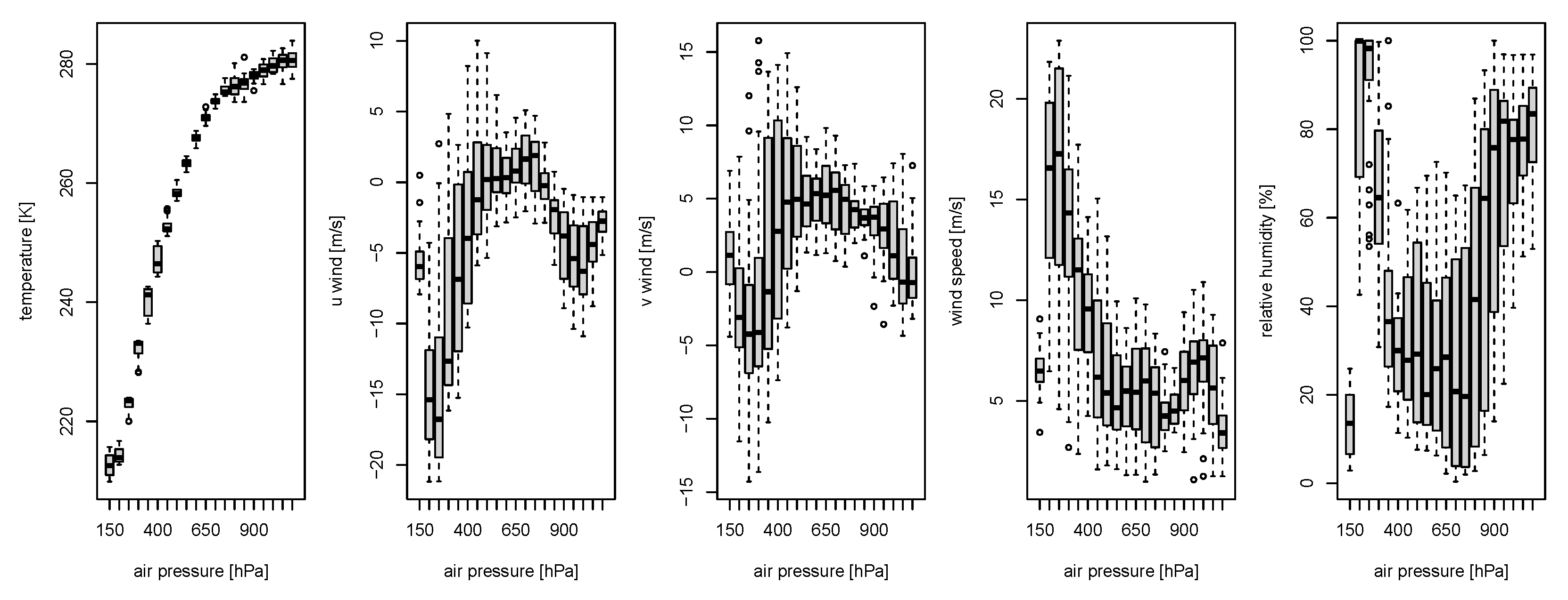
Figure 4 depicts using boxplots how weather variables for the given data sample, namely temperature (K), U-wind (m/s), V-wind (m/s), wind speed (m/s), and relative humidity (%), behave along with the air pressure. Temperature data in Figure 4 presents a noticeable trend with altitude but not for wind or relative humidity, in line with the international standard atmosphere model. We will discuss this trend model of temperature later in Section 3.2.
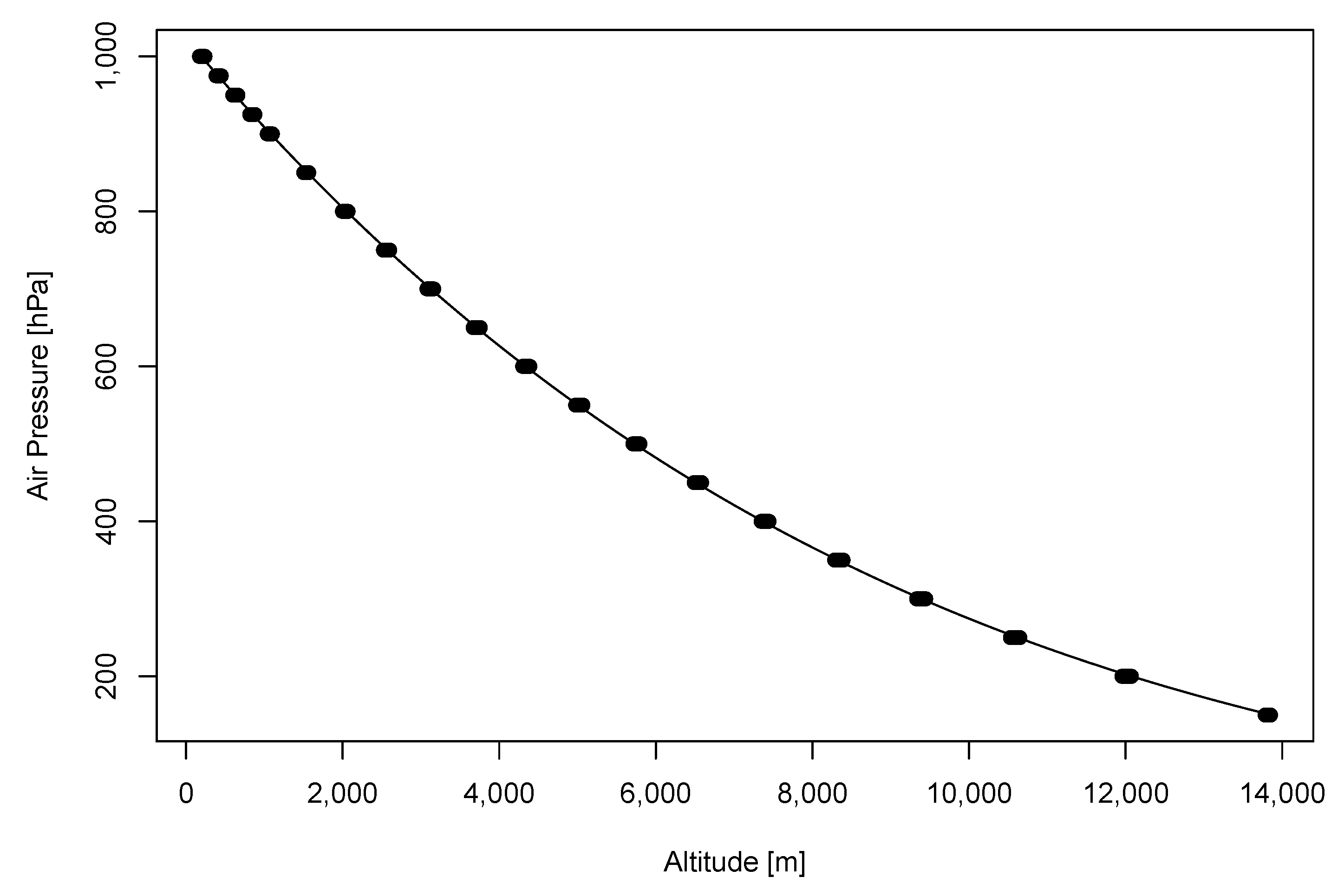
Air pressure (hPa) in GFS depicted with dots as the function of the altitude in Figure 5 presents a classical pattern. Thus, we can apply the exponential atmosphere formula [23].
z ^ p ( s i ) = β ^ 0 ( 1 s i , 3 / β ^ 1 ) β ^ 2 .
The curve results for our data are fitted by the OLS into z ^ P ( s i ) = 1022.79 ( 1 s i , 3 / 49 , 262.75 ) 5.80 . We will continue with the estimated air pressure from altitude as the residuals are within 4 hPa. We have tried other, more sophisticated regression techniques, but the current exponential formula is simple and provides acceptable accuracy.
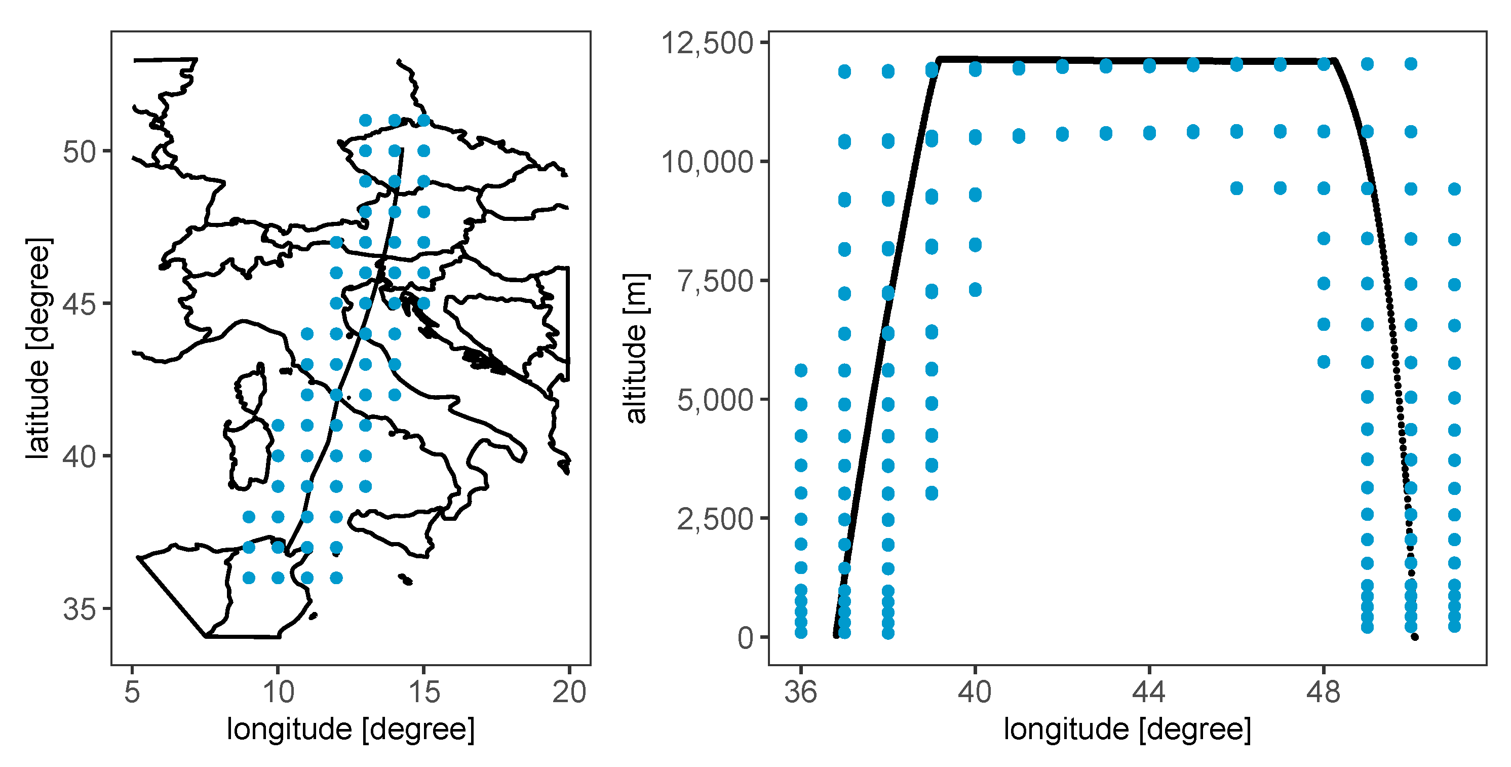
In the next sections, we provide details in the various interpolations methods used for weather variables. In order to evaluate them, we examine the trajectory from Prague to Tunis. Some of the techniques are extremely time-consuming. For the sake of computational time, the GFS data are reduced along the trajectory to be as small as possible. The data are reduced as an “arc” shape along the trajectory, as shown in Figure 6. From the horizontal perspective, the data are the union of blocks with the sizes of two degrees along the trajectory; from the vertical perspective, data below the trajectory are removed to guarantee a fast computation. A smaller data set is indeed important for Kriging and RBF. Other methods, such as linear interpolation, decision trees, and neural networks, do not require small data; still, we kept the reduced dataset for a fair comparison. The ranges of all the variogram models in Kriging are fixed as one to fit with the local GFS data and avoid singularities in the covariance matrices.

3. Interpolation Methods

In the following, we introduce interpolation methods: linear interpolation, Kriging (Ordinary Kriging and Universal Kriging), RBF methods, feedforward neural networks, and decision trees with bagging and gradient boosting machines to interpolate spatial dimensions. As already stated in the previous section, we consider these methods because they are widely used in the variety of applications. For example, linear interpolation is often used for weather information in the trajectory optimization [8], applications of Kriging on meteorological data [12,24], soil organic matter content [13], RBF methods on air pollution [25], neural network on dissolved gas in the dam’s reservoir [15], surface daily minimum temperature [16], and decision trees on seabed sand content [17,18].

3.1. Linear Interpolation

For simplicity and completeness, let us first consider a one-dimensional setting depicted in Figure 7.
Suppose s i , 1 , s j , 1 { s 1 , 1 , , s n , 1 } are locations of two closest observations to s 0 , 1 in the Euclidean sense. Linear interpolation estimates the unknown value of the variable of interest z ( s 0 , 1 ) by the weighted average of closest neighbours z ( s i , 1 ) and z ( s j , 1 ) as
z ^ ( s 0 , 1 ) = s j , 1 s 0 , 1 s j , 1 s i , 1 z ( s i , 1 ) + s 0 , 1 s i , 1 s j , 1 s i , 1 z ( s j , 1 ) .
For multiple dimensions, ref. [7,8] interpolate first vertically then horizontally, and the detailed steps are as follows.
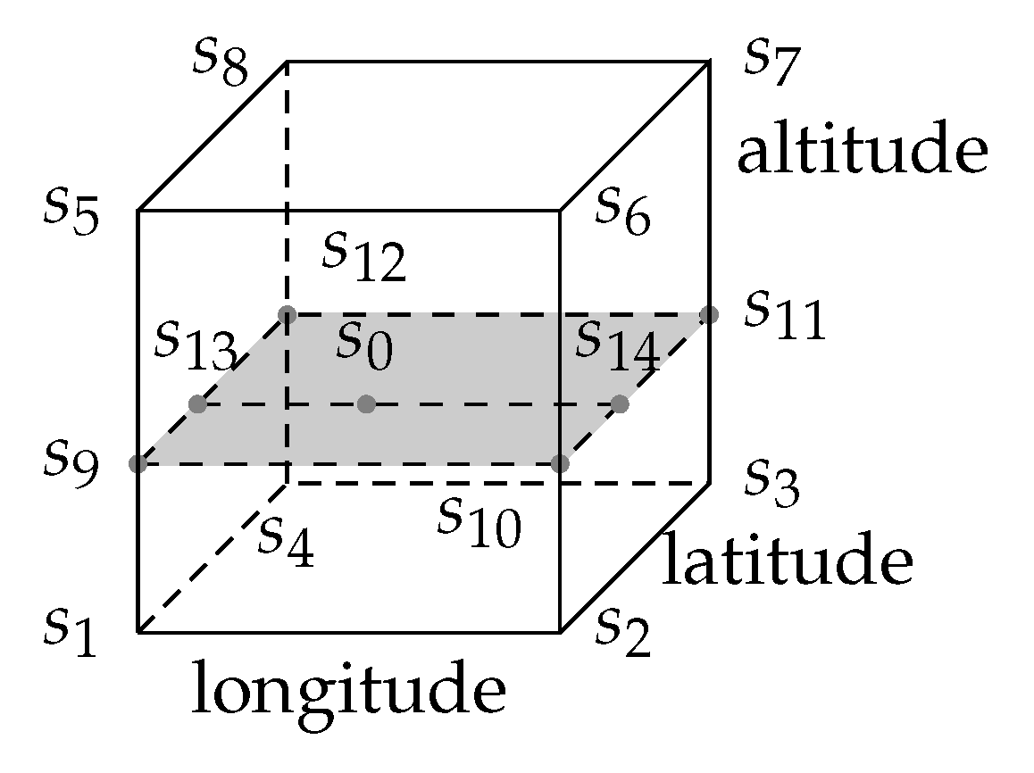
Suppose s 1 , s 2 , , s 8 in Figure 8 are the observations, and s 0 lies on the grey plane. The value at the intermediate locations ( s 9 , s 10 , s 11 , s 12 ) and ( s 13 , s 14 ) are to be interpolated first. The estimations are first identified at locations on the grey plane, specifically s 9 , s 10 , s 11 , and s 12 , thus with the same altitude s 0 , 3 as s 0 . An estimation z ^ ( s t ) for t { 9 , 10 , 11 , 12 } can be calculated from z ( s t 8 ) and z ( s t 4 ) with one-dimensional linear interpolation as s t 8 , 1 = s t 4 , 1 = s t , 1 and s t 8 , 2 = s t 4 , 2 = s t , 2 ,
z ^ ( s t ) = s t 4 , 3 s t , 3 s t 4 , 3 s t 8 , 3 z ( s t 4 , 3 ) + s t , 3 s t 8 , 3 s t 4 , 3 s t 8 , 3 z ( s t 8 , 3 ) .
This three-dimensional interpolation is thus reduced to a two-dimensional problem, with the points lying on the grey plane in Figure 8. Afterward, we interpolate z ^ ( s 13 ) and z ^ ( s 14 ) along the latitude,
z ^ ( s 13 ) = s 12 , 2 s 13 , 2 s 12 , 2 s 9 , 2 z ^ ( s 12 , 2 ) + s 13 , 2 s 9 , 2 s 12 , 2 s 9 , 2 z ^ ( s 9 , 2 ) ,
z ^ ( s 14 ) = s 11 , 2 s 14 , 2 s 11 , 2 s 10 , 2 z ^ ( s 11 , 2 ) + s 14 , 2 s 10 , 2 s 11 , 2 s 10 , 2 z ^ ( s 10 , 2 ) .
Finally, z ( s 0 ) can be interpolated along the longitude dimension with z ^ ( s 13 ) and z ^ ( s 14 ) ,
z ^ ( s 0 ) = s 14 , 1 s 0 , 1 s 14 , 1 s 13 , 1 z ^ ( s 14 , 1 ) + s 13 , 1 s 0 , 1 s 14 , 1 s 13 , 1 z ^ ( s 13 , 1 ) .
Linear interpolation interpolates dimension by dimension and, apparently, the interpolation values can vary when the order of interpolating dimensions changes.
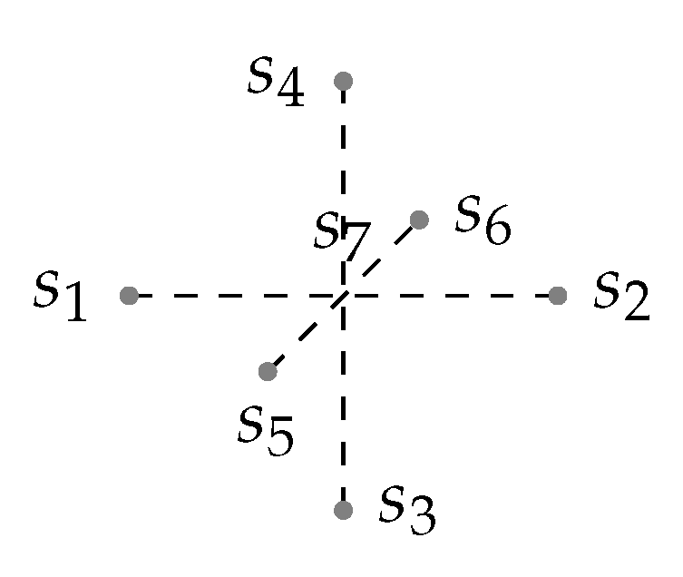
When we, however, employ Leave-One-Out Cross-Validation (LOOCV) for linear interpolation later in Section 3.4, we choose a slightly different way from the one in Figure 8 due to the one observation being removed from the grid. A weighted average of six nearest observations in three coordinates is used as an estimate for z ^ ( s 7 ) | z ( s ) \ z ( s 7 ) in Figure 9, where z ( s ) \ z ( s 7 ) means z ( s ) with z ( s 7 ) removed. In this way, the weights can be calculated separately on longitude, latitude, and altitude based on the one-dimensional linear interpolation,
longitude : z ^ ( s 7 ) = w ^ 2 z ( s 2 ) + w ^ 1 z ( s 1 ) = s 2 , 1 s 7 , 1 s 2 , 1 s 1 , 1 z ( s 2 ) + s 7 , 1 s 1 , 1 s 2 , 1 s 1 , 1 z ( s 1 ) ,
latitude : z ^ ( s 7 ) = w ^ 4 z ( s 4 ) + w ^ 3 z ( s 3 ) = s 4 , 2 s 7 , 2 s 4 , 2 s 3 , 2 z ( s 4 ) + s 7 , 2 s 3 , 2 s 4 , 2 s 3 , 2 z ( s 3 ) ,
altitude : z ^ ( s 7 ) = w ^ 6 z ( s 6 ) + w ^ 5 z ( s 5 ) = s 6 , 3 s 7 , 3 s 6 , 3 s 5 , 3 z ( s 6 ) + s 7 , 3 s 5 , 3 s 6 , 3 s 5 , 3 z ( s 5 ) .
The estimate is made by averaging the values of these neighbours,
z ^ ( s 7 ) | z ( s ) \ z ( s 7 ) = k = 1 6 w ^ k z ( s k ) k = 1 6 w ^ k .
For the points on faces, edges, or vertices, the estimation is made by averaging values of available neighbours. The RBF method is a flexible interpolation technique that interpolates through basis functions, also known as kernels, κ ( s , s ) = ψ ( s ) , ψ ( s ) , which are dot products in the feature space with a map ψ . The so-called “kernel trick” allows the definition of kernels without specifying the mapping ψ ( s ) . This paper applies the Gaussian kernel κ ( s i , s j ) = exp { ε s i s j 2 2 } , where s i s j 2 = p = 1 3 s i , p s j , p 2 is the Euclidean distance between locations s i and s j , and ε is the shape parameter that controls the range. RBF methods interpolate through a linear combination of kernels as z ( s ) = K ( s , s ) · w , where w = ( w 1 , , w n ) is a vector of weights and the kernel matrix K ( s , s ) has entries { K } i , j = κ ( s i , s j ) = κ ( s i s j 2 ) , i , j = 1 , , n . A kernel κ ( s i , s j ) is said to be strictly positive definite [26] if the kernel matrix K is strictly positive definite for any set s = { s 1 , , s n } . The Gaussian kernel is a strictly positive definite kernel, thus allowing inversion. Weights w and prediction at location s 0 are therefore estimated as
w ^ = K 1 ( s , s ) z ( s ) ,
z ^ ( s 0 ) = K ( s 0 , s ) w ^ = K ( s 0 , s ) K 1 ( s , s ) z ( s ) ,
The accuracy of the interpolation and RBF method strongly depends on the parameter ε in the Gaussian kernel. Figure 10 shows interpolation results of wind speed as a surface with three different ε , which controls the locality of the estimation. For small ε , the Gaussian kernel decays slowly, and the interpolation surface becomes flat; if ε is large, interpolation relies on close neighbours, and the corresponding interpolation surface is noisy.
Besides ε , the estimation of z ( s 0 ) depends on neighbours weighted according to the distance. As written in Section 2, along the vertical direction, the data is denser. A scaling factor b is used to convert altitude from meter to the same scale as longitude and latitude, s i , 3 * = s i , 3 / b , and we continue interpolating with s i , 3 . Finally, parameters ε and b are found via minimization of the 10-fold cross-validation Mean Squared Error (cv-MSE),
cv - MSE = 1 n i = 1 n z ( s i ) z ^ ( s i ) 2 ,
where z ^ ( s i ) are estimated by the train set and evaluated by the test set at each fold. The optimal parameters are searched to minimize cv-MSE for temperature, wind speed, and relative humidity with a simulated annealing algorithm, see [27]. Finally, the optimal in the sense of the smallest cv-MSE of pairs of ε and b are ( ε = 0.23 , b = 801.87 ) for temperature, ( ε = 0.51 , b = 800.00 ) for wind speed, and ( ε = 0.27 , b = 800.00 ) for relative humidity.

3.2. Kriging

Kriging is similar to the RBF method through the utilization of kernels, but differs in finding appropriate parameters. In contrary to the search for ε in the RBF method, Kriging estimates parameters using covariance structure. In this section, we will first discuss the Ordinary Kriging and extend to the Universal Kriging. Furthermore, we also discuss how to bridge the different units of coordinate variables, longitude (in degrees), latitude (in degrees), and altitude (in meters).

3.2.1. Estimation of Kriging Weights

An in-depth discussion about Kriging can be found in [28,29]; for that reason, we concentrate only on the points that are relevant for our application of flight routing. Ordinary Kriging seeks to find weights w to obtain Z ( s 0 ) = i = 1 n w i Z ( s i ) through the minimization of the Mean Squared Error, MSE = E { Z ( s 0 ) Z ^ ( s 0 ) } 2 , under the assumption of second-order stationarity, E { Z ( s i ) } = E { Z ( s j ) } = μ and Var { Z ( s i ) } = Var { Z ( s j ) } . We stress here that capitalized Z corresponds to random variables, with lower-case z standing for realizations. By setting the first-order derivative MSE w equal to zero, we have the representation of the weights,
w ^ = Var { Z ( s ) } 1 Cov { Z ( s 0 ) , Z ( s ) } ,
where Z ( s ) = Z ( s 1 ) , Z ( s 2 ) , , Z ( s n ) .
Furthermore, the prediction of Z ( s 0 ) at the unobserved location is given through
Z ( s 0 ) = Z ( s ) w ^ = Z ( s ) Var { Z ( s ) } 1 Cov { Z ( s 0 ) , Z ( s ) } .
In order to obtain the interpolated value z ^ ( s 0 ) , all the theoretical covariances in (16) should be replaced by their empirical counterparts. Thus, we need an estimate of the covariance Cov Z ( s i ) , Z ( s j ) between Z ( s i ) and Z ( s j ) , which, assuming local spatial homogeneity, can be represented by a covariance function of the distance h = s i s j 2 between locations s i and s j :
C ( h ) = Cov Z ( s i ) , Z ( s j ) .
Covariance Cov { Z ( s i ) , Z ( s j ) } is a measure of the similarity between variables Z ( s i ) and Z ( s j ) . The farther the two points are, the smaller the empirical covariance is, of course, with the fixed scale. Points far away are assumed to have a more negligible impact on estimation than nearer observations. Corresponding covariance function C ( h ) is also a non-increasing function with h. We define the semivariance, and its relation to C ( h ) is as follows,
γ ( h ) : = 1 2 Var { Z ( s + h ) Z ( s ) } = C ( 0 ) C ( h ) ,
The empirical counterpart of γ ( h ) is given through
γ ^ z ( h ) 1 2 | N s ( h ) | s i , s j N s ( h ) z ( s i ) z ( s j ) 2 ,
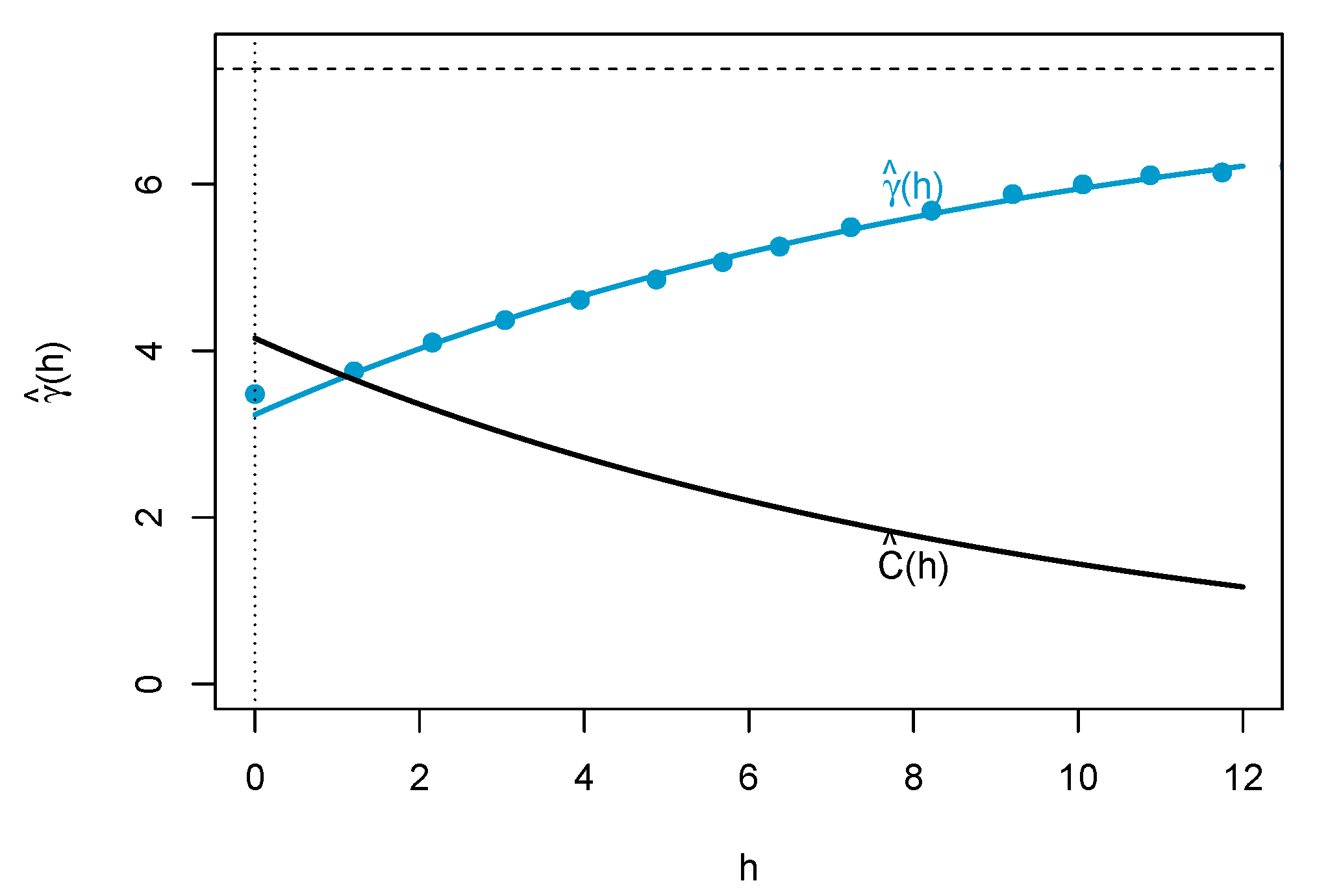
where N s ( h ) is the set of locations with distance h. With γ ^ z ( h ) being evaluated at different h, we can use variogram models to fit γ ^ ( h ) . Figure 11 shows blue points γ ^ z ( h ) calculated with (19). It is important to note that γ ^ ( h ) can be affected by the unit of z i but unaffected by the unit of distance h. There are many parametric models for modelling the semivariance, such as the spherical model or Gaussian model. Figure 11 presents an exponential model estimated via OLS with the nugget effect, γ ^ ( h ) = 7.38 4.15 e h / 9.46 and C ^ ( h ) = 4.15 e h / 9.46 when h > 0 . Below, we summarize computation steps of the Kriging estimation:
  • Calculate empirical semivariance γ ^ z ( h ) with (19);
  • Fit a semivariance model γ ^ ( h ) from γ ^ z ( h ) ;
  • Find covariance function C ^ ( h ) from γ ^ ( h ) with (18);
  • Calculate covariance Cov ^ { Z ( s ) , Z ( s ) } and Cov ^ { Z ( s 0 ) , Z ( s ) } with (17);
  • Estimate Z ( s 0 ) with (16).

3.2.2. Trend

Ordinary Kriging, discussed in the previous section, assumes stationarity, which can be relaxed by including trend as a function of location s, μ ( s ) = E { Z ( s ) } , also known as Universal Kriging. After detrending, Z * ( s ) = Z ( s ) μ ( s ) remains stationary; accordingly, the model for Z ( s 0 ) becomes
Z ( s 0 ) = μ ( s 0 ) + Z * ( s ) Cov { Z * ( s ) , Z * ( s ) 1 Cov { Z * ( s 0 ) , Z * ( s ) } .
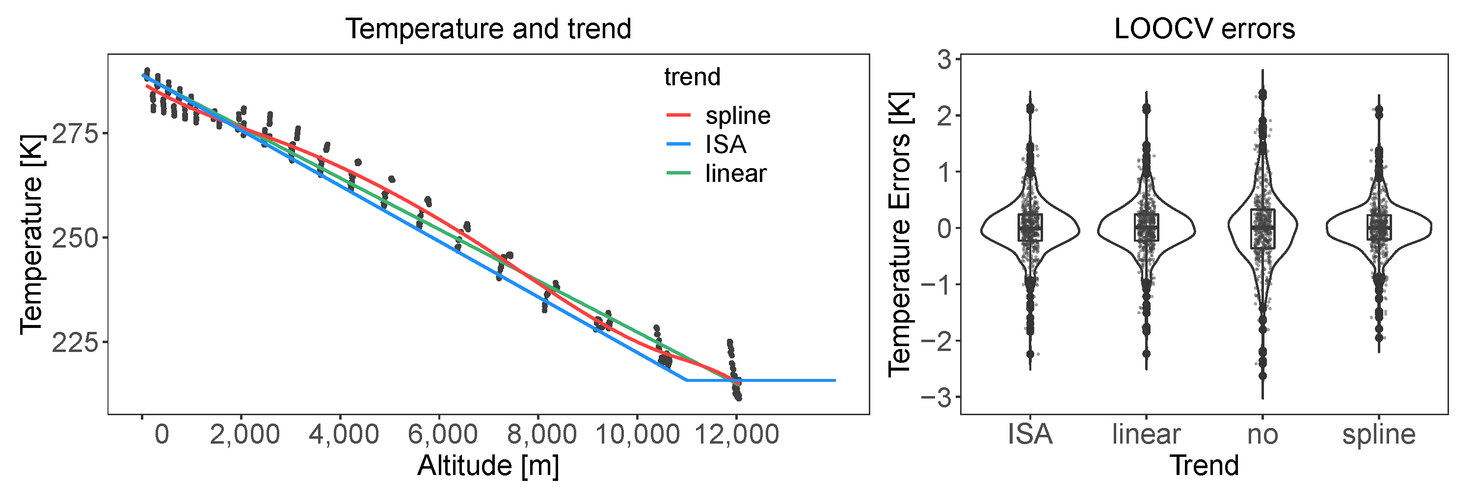
Usually, trend μ ( s ) is unknown and needs to be estimated. Among the weather variables in Figure 4, temperature presents high dependence on altitude, while wind and relative humidity reveal no obvious trend. For this reason, we use ordinary Kriging for all the variables except temperature. We compare the following four classical trend models in Figure 12, which we use for temperature:
  • No trend or Ordinary Kriging as in (16).
  • Cubic spline [30]: z ^ Temp ( s i ) = β ^ 0 + β ^ 1 s i , 3 + β ^ 2 s i , 3 2 + β ^ 3 s i , 3 3 + β ^ 4 ( s i , 3 ξ 1 ) 3 + β ^ 5 ( s i , 3 ξ 2 ) 3 + β ^ 6 ( s i , 3 ξ 3 ) 3 , where z Temp ( s i ) is the temperature at s i and s i , 3 denotes the altitude at location s i . Knots are set as ( ξ 1 , ξ 2 , ξ 3 ) = (3000, 7000, 10,500) m.
  • Linear regression: z ^ Temp ( s i ) = β ^ 0 + β ^ 1 s i , 3 .
  • International Standard Atmosphere (ISA) assumes a piecewise linear function for temperature [23].
z ^ Temp ( s i ) = β ^ 0 + β ^ 1 s i , 3 , 0 < s i , 3 < 11 , 000 , β ^ 3 , 11 , 000 s i , 3 < 20 , 000 .
From the right panel of Figure 12, we can see no notable improvement from no trend to trend models, no matter what kind of trend model being used. The physical model ISA (International Standard Atmosphere) and spline model are slightly better than no trend model. We utilize Ordinary Kriging in the following Section 3.5 and Section 4, assuming that the GFS data is second-order stationary and has a constant but unknown mean μ .

3.2.3. Scaling Factor and Function

Unit transformation is needed to bridge the gap among coordinate variables, longitude (in degrees), latitude (in degrees), and altitude (in meters). A degree of longitude corresponds around 100 km, but this unit conversion has problematic interpolation. Observations in the vertical direction are much denser than in the horizontal direction, so the estimated value will be equivalent to the ones of the neighbouring altitudes. The first row in Figure 13 shows that interpolation results deviate heavily from longitudinal and latitudinal observations. For this reason, the initial conversion will also generate a much higher cross-validation error. Besides these problems, the computation becomes unstable when distances over one million meters are converted from the degree, and C ^ ( h ) often becomes singular.
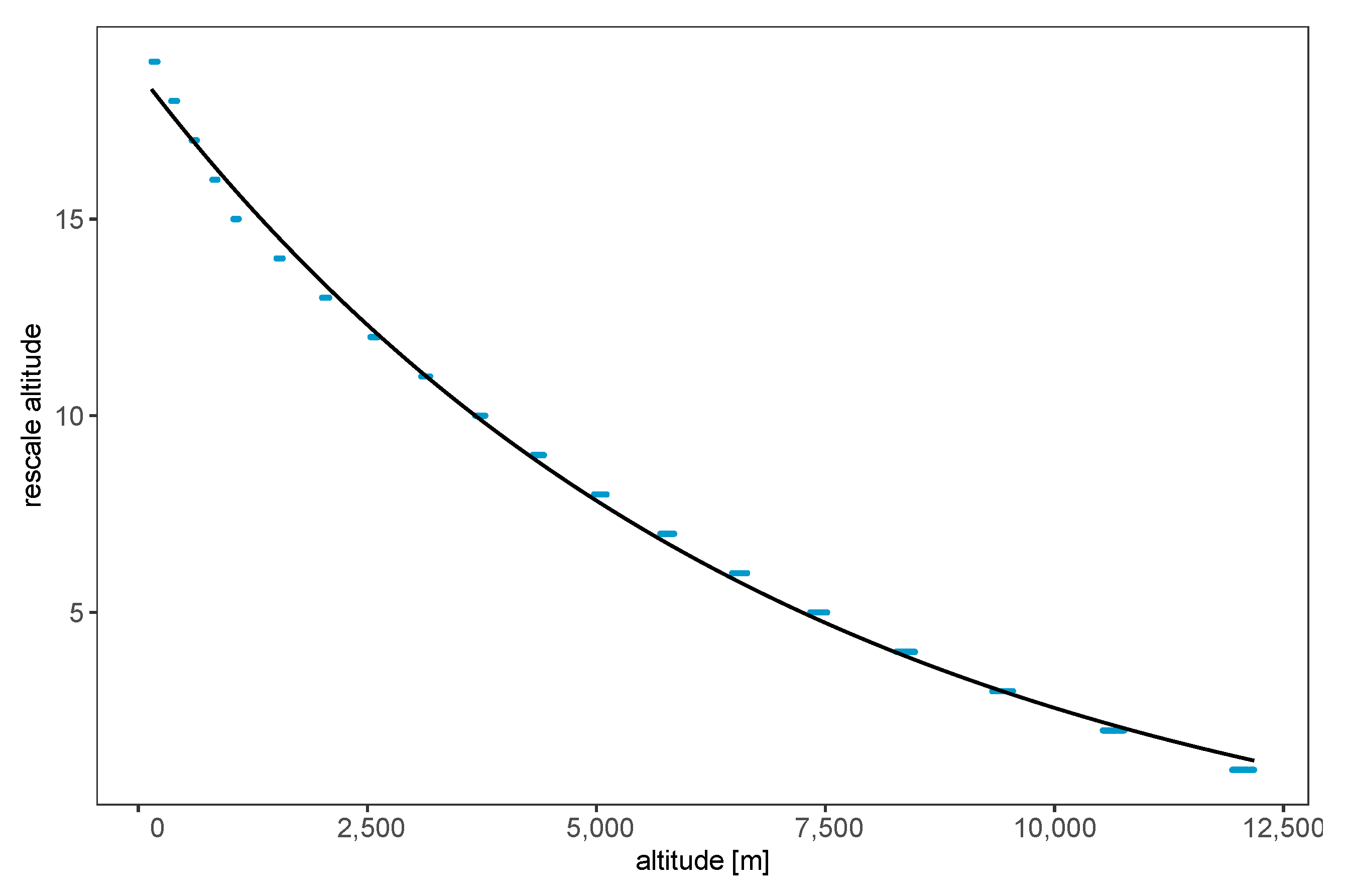
In contrast, the second row in Figure 13 interpolates by introducing a scaling factor. We divide the altitude by this scaling factor, which converts altitude from meter to the same scale as longitude and latitude. This scaling factor will improve the interpolation results and generate a much smaller cross-validation error. Therefore, which scaling function to use is still an open question. To allow for the variogram function to have the same weight for vertical and horizontal neighbours, we rescale the altitude s i , 3 as one unit distance s i , 3 * { 1 , 2 , 3 , , 20 } , which becomes the same as the horizontal distance. The scatterplot of s i , 3 * and s i , 3 can be seen from Figure 14, and they are fitted with OLS as
s ^ i , 3 * = 2.36 + 21.10 exp s i , 3 6884.60 ,
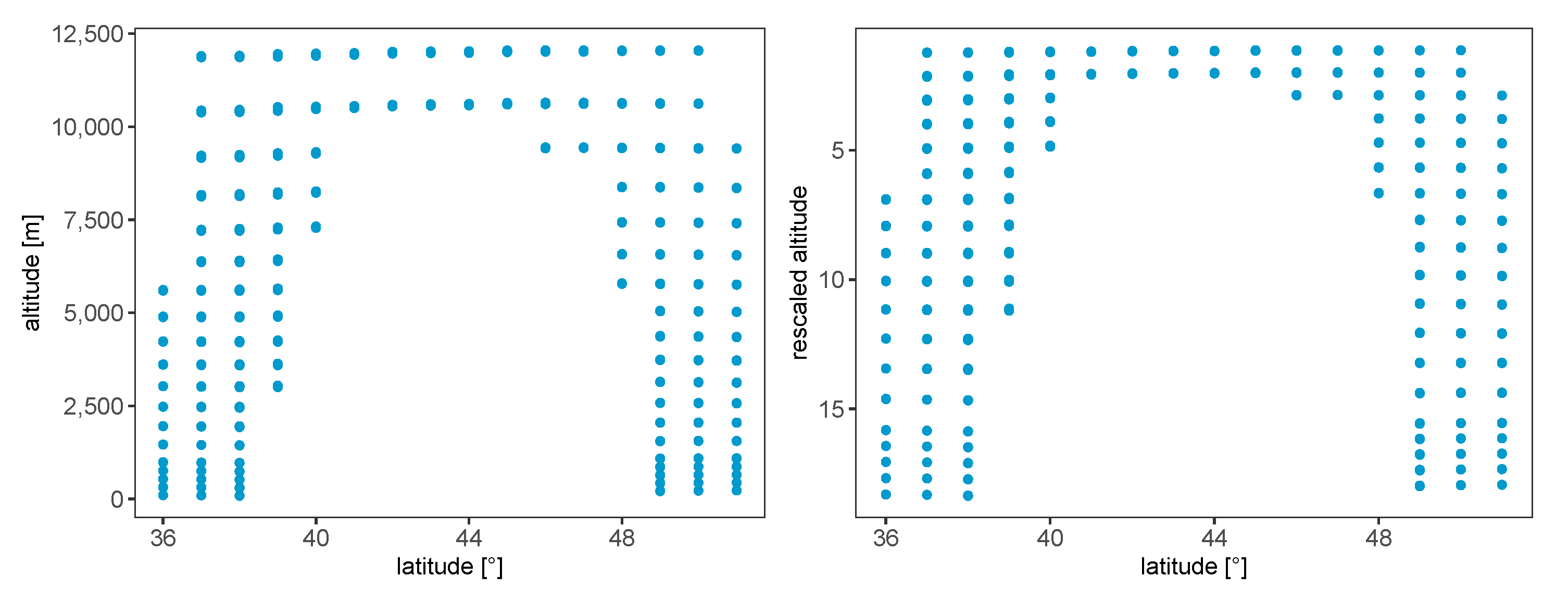
also the curve in Figure 14. Figure 15 shows the original GFS data on the left panel and the rescale data on the right.
The semivariance models γ ^ ( h ) for temperature, wind speed, and relative humidity is depicted in Figure 16, with Gaussian semivariance model and scaling function (22).

3.3. Feedforward Neural Networks

In line with the current strand of research, we also consider a neural network for interpolation. Discussion of this section mainly refers to [31,32]. For a brief recall, a network regression fits f N N ( s ; W ) , where s is locations as input and W is a matrix of weights for all layers. Parameters W are estimated by minimizing cost function J ( s , W ) ,
W = arg min W J ( s , W ) .
We used cv-MSE as in (14) as a cost function; to be more specific,
J ( s , W ) = cv - MSE = 1 n i = 1 n z ( s i ) f N N ( s i ; W ) 2 ,
where n is the sample size for train/test set, z ^ ( s i ) is an estimation using a deep feedforward neural network with the weights being updated using the back-propagation. In this study, we used tanh ( x ) = sinh x cosh x = exp ( x ) exp ( x ) exp ( x ) + exp ( x ) as an activation function.
We used a deep feedforward network estimation implemented by TensorFlow [33] and Keras [34]. Figure 17 and Table 1 present a comparison of cv-MSE in (24) with various model sizes. The cv-MSE is evaluated on the test set, which contains 20% of the data. The input layer has three units for all models, corresponding to three dimensions in space, longitude, latitude, and altitude. The output layer predicts the weather variables. A deeper network attains smaller cv-MSE faster for temperature and wind speed but not necessarily for relative humidity. The cv-MSE differences are not discernible after sufficient epochs in Figure 17 and can be seen in Table 2. A deeper network can have smaller cv-MSE, even if compared with the perceptron for the last epochs. Therefore, we apply the deep neural network with four layers.
To avoid overfitting, we added the L 2 penalty on the weight parameter to the deep network, with the final objective function being
J ˜ s , W = α 2 W W + J s , W .
Penalty α is searched on a grid of ( 0 , 0.001 , 0.01 , 0.1 , 1 , 10 , 100 , 1000 ) with cv-MSE results as listed in Table 2. For example, setting α as 0.01 would generate the smallest cross-validation error for temperature. The final model is regularized with α = ( 0.01 , 1 , 1 ) for temperature, wind speed, and relative humidity. Therefore, the feedforward neural network evaluated in Section 3.4 is a regularized deep network with four layers, with 500, 300, 100, and 50 units, respectively (the model in the last row of Table 1).

3.4. Decision Tree

Classification or regression trees can perform non-linear regression, thus can perfectly serve for interpolation as well, see [32,35,36]. For implementation, we refer to [37]. A decision tree can be defined as the sum of piecewise functions,
T ( s ; Θ ) = q = 1 Q c q 1 { s R q } ,
where 1 { · } is the indicator function, Q denotes the number of trees, and Θ = { R q , c q } q = 1 , , Q (see [35]) with { R q } being disjointed regions and c q are constants corresponding to region R q . Regions are selected by minimizing Residual Sum Squared (RSS) q = 1 Q i R q { z ( s i ) T ( s i ; Θ ^ ) } 2 . For every possible split, a partition is made where minimal RSS can be attained.
Bagging and boosting are applied in this section to improve the accuracy of the regression tree, which may have a large variance, and bagging improves prediction accuracy by averaging the prediction from a bunch of trees. For bagging with B subsamples, decision trees are estimated as T 1 ( s , Θ ^ 1 ) , , T b ( s , Θ ^ 2 ) , , T B ( s , Θ ^ B ) using B sample sets, and then they are averaged for a bagged model [35],
f ^ bag ( s ) = 1 B b = 1 B T ^ b ( s ) .
Besides bagging, boosting can learn and update the previous tree model. Boosting uses the sum of weak learners to construct a strong prediction model. Gradient Boosting Machines (GBM) boost by combining a gradient descent algorithm and modelling tangent of cost function then updating models towards the optimal. A gradient boosting machine estimates f gbm ( s ) by minimizing the cost function with regularized objective [38],
f ^ gbm ( s ) = arg min f gbm ( s ) L { z , f gbm ( s ) } + Ω ( f gbm ) ,
where Ω adds the penalty and L { z , f gbm ( s ) } is a loss function, in this paper as Root Mean Square Error, RMSE = 1 n i = 1 n z ( s i ) f ^ gbm ( s i ) 2 . We restrict f gbm ( s ) to be a function with parameters f gbm ( s , { β m , Θ m } 1 M ) = i = 1 M β m T ( s ; Θ m ) with T ( s ; Θ ) being a decision tree in (26), also served as a weak learner. Ref. [36] proposed a steepest descent algorithm to update f gbm ( s ) step by step and use trees to approximate the gradients of the loss function. A grid search procedure with a minimal 10-fold cross-validation RMSE selects the hyperparameters, including the learning rate of ( 0.1 , 0.05 , 0.05 ) , maximum tree depth of ( 20 , 10 , 10 ) , a minimum number of observations within a node as ( 3 , 3 , 3 ) , L 1 norm regularization parameter as ( 100 , 0 , 0 ) , and L 2 norm penalty parameter as 0 for temperature, wind speed, and relative humidity. The learning process to update f gbm ( s ) can be seen in Figure 18.

3.5. Comparison of Methods

To summarize, all the methods aim to construct a complex function for interpolation but with different approaches. Both the RBF method and Kriging construct a surface with kernels, which maps s into a higher dimensional space. Estimation surface as z ( s 0 ) = K ( s 0 , s ) w can be thought of as a linear regression in the higher dimensional feature space. The difference between the RBF method and Kriging lies in the way to estimate parameters of kernels. Machine learning methods applied in this paper interpolate by network or tree structure. Parameters are fitted by minimizing the loss function L z , f ( s ) , which for all the methods is almost the same, up to regularization. Both machine learning methods require derivatives of cost function L z , f ( s ) to update parameters. Neural network updates by backpropagation and GBM updates f ( s ) by estimating gradient with a decision tree.
This section evaluates and compares by the leave-one-out Mean Squared Error (loo-MSE),
loo - MSE = 1 n i = 1 n z ( s i ) z ^ ( s i ) | z ( s ) \ z ( s i ) 2 ,
where z ( s ) \ z ( s i ) , as mentioned before, corresponds to the data with observation z ( s i ) being removed, z ^ ( s i ) | z ( s ) \ z ( s i ) is the estimation with observation z ( s i ) being removed, and z ( s i ) z ^ ( s i ) | z ( s ) \ z ( s i ) is the cross-validation error.
Data preprocessing and hyperparameters searching for each method are in Section 3. Cross-validation usually splits the data into train, test, and validation sets. We consider only train and test sets, with no validation set in Table 3, because we can fit models and interpolate with the same data set in SOPHIA. Errors by test set can evaluate the methods when interpolating trajectories. We have a more realistic assessment of the Kriging method in Section 4 with balloon data as the validation set.
Table 3 presents loo-MSE results by these methods. The RBF method and Kriging have the smallest loo-MSE for temperature, wind speed, and relative humidity. The statistical learning methods such as neural networks and bagging have less satisfactory loo-MSE. Actually, the trajectory with GBM interpolation does not land on the runway, resulting from not even continuous weather values (see Figure 19). Neural networks make SOPHIA often abort with an error message of an invalid aircraft state. Ordinary Kriging and the RBF method are the potential methods to interpolate the weather variables along the trajectory. In Section 4 we experiment with Ordinary Kriging due to its comparable loo-MSE to the RBF method for wind speed and relative humidity. Additionally, the RBF method is four times slower than Ordinary Kriging when integrating into SOPHIA. Ordinary Kriging takes 23 h to generate a trajectory, while the RBF method can take up to 4 days. As we see in Section 4, Ordinary Kriging can have minor errors when validated with balloon data. These errors have a trivial impact on the trajectories, according to the simulation results.

4. Monte Carlo Simulation

As discussed in the introduction, we need a perfect understanding of the weather conditions for trajectory planning. Considering that all the data sources deliver very sparse data information, interpolation is needed, which was discussed in the previous sections. Nevertheless, what happens if the data source is not perfectly reliable, but affected by measurement or modelling errors? Earlier, we concentrated on the GFS data source, considering it the best available source for our needs, but it is known that it is not a perfect weather data source either, nor is using further models for interpolation. We hope to investigate the effect of this inaccuracy on SOPHIA in this section by adding simulated errors to the GFS data and running Monte Carlo simulations. These simulation results can reveal how the errors of GFS data and Kriging interpolation impact the trajectory. Our choice of the interpolation method has been clearly motivated in the previous sections. The steps, which are explained in detail later, are as follows:
  • We regard the data collected by the releasing balloons as the accurate weather data and compare the interpolation results by the Ordinary Kriging with GFS data as input. The errors are defined as the difference between the balloon data z j , bal and the interpolated values by Ordinary Kriging with the GFS inputs z ^ j , GFS , Kriging . For j { Temp , U - wind , V - wind } ,
    e ^ j = z j , bal z ^ j , GFS , Kriging ;
  • Quantify and investigate the dependency among the errors e ^ Temp , e ^ U - wind , and e ^ V - wind ;
  • Select bivariate copulas such that
    F ^ j ( e ^ j ) , F ^ k ( e ^ k ) C j , k ( · , · ) ;
    where the empirical margins F ^ j ( x ) = 1 n + 1 i = 1 n I { x e ^ j , i } with j k and j , k { Temp , U - wind , V - wind } ;
  • Generate uniform pseudo-noise u ˜ Temp , u ˜ U - wind , u ˜ V - wind based on the selected copula model;
  • Generate random errors e ˜ j = F ^ j 1 ( u ˜ j ) with j { Temp , U - wind , V - wind } . In this step, instead of using empirical distribution function, the kernel smoothed one is used in order to avoid purely bootstrapped observations;
  • Generate weather scenarios with GFS data and errors where weather data at each location of GFS grid has the simulated error added,
    z ˜ Temp = z Temp , GFS + e ˜ Temp , z ˜ U - wind = z U - wind , GFS + e ˜ U - wind , z ˜ V - wind = z V - wind , GFS + e ˜ V - wind ;
  • Calculate the trajectories with Ordinary Kriging interpolations and simulated weather scenarios,
    SOPHIA ( z ˜ Temp , z ˜ U - wind , z ˜ V - wind ) .
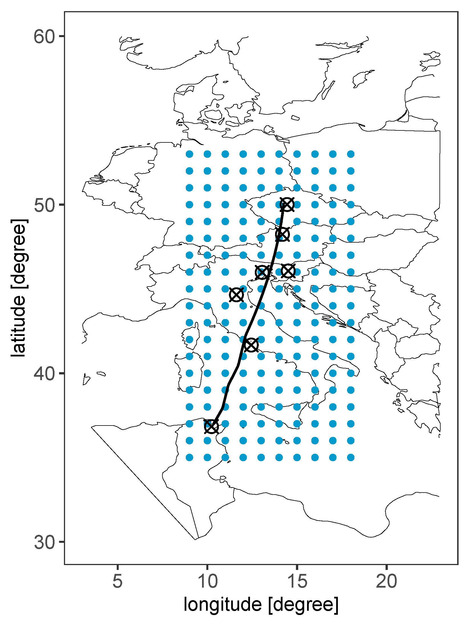
The errors in the first step are the differences between the balloon data and the Kriging interpolation with the GFS inputs. Figure 20 has the GFS data as blue points and weather stations as the black points, which are no more than 1.5 km away from the trajectory (minimal distance). We assume the balloons are released at the exact location of the weather stations and will not drift away. We only consider the data which are lower than 150 hPa. Three snapshots from 3 to 4 November 2018 are used to increase the error sample size; see Figure 21 regarding the distributions of errors from three snapshots.

4.1. Dependency

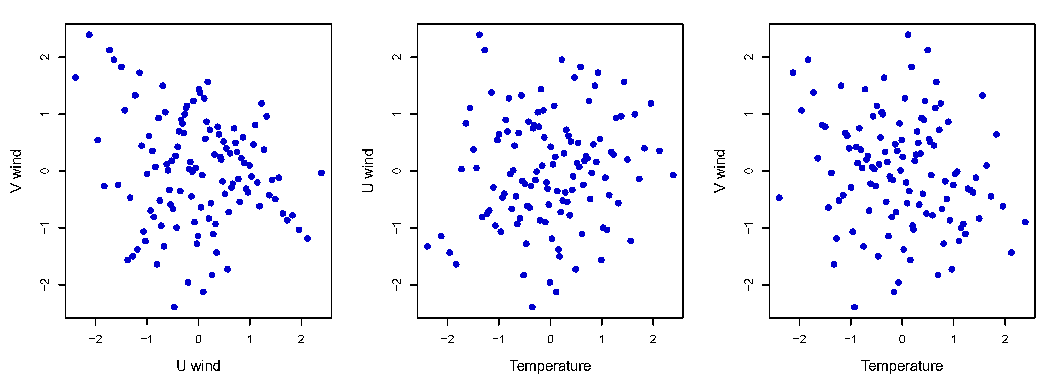
Weather variables in the real world can be naturally dependent, such as temperature and wind, which both GFS and balloon data confirm. However, the errors can have dependencies as different as the weather value themselves. Figure 22 depicts the normal scores of errors for all pairs { ( Φ 1 ( e ^ U - wind ) , Φ 1 ( e ^ V - wind ) } , { Φ 1 ( e ^ Temp ) , Φ 1 ( e ^ U - wind ) } and { Φ 1 ( e ^ Temp ) , and Φ 1 ( e ^ V - wind ) } , with Φ ( · ) being the CDF of the standard normal distribution. This figure shows a weak correlation among these errors, probably resulting from correlation deprived by GFS data from the balloon data.
Both Spearman’s ρ and Kendall’s τ [39] are presented in Table 4 to quantify these results, where ρ is the measure of monotone dependency and τ is a measure of concordance with the paired signs. The rank correlation results in this table confirm weak monotone dependence between the errors.

4.2. Modelling the Dependency

Even if these errors are weakly correlated, a joint multivariate distribution is needed to model their dependency structure and generate weather scenarios for Monte Carlo simulation. As the flexible tool for dependence modelling, the copula is commonly applied to model the multivariate distribution of weather variables. Ref. [40] model several meteorological variables, including maximum and minimum temperatures, sea-level pressure, maximum wind speed, and precipitation, with the Gaussian copula. Ref. [41] applies copula to describe the dependence between temperature and precipitation with daily data collected by eastern and western Mediterranean stations. According to Sklar’s theorem [42], a bivariate distribution can be expressed as a copula of margins, H j , k ( e j , e k ) = C j , k { F j ( e j ) , F k ( e k ) } . Copula enables us to model the multivariate distribution of random variables by separating the marginal distribution and dependency structure of these margins. For recent developments in the field of the copula, the interested reader can refer to [43].
This paper focuses on the Gaussian, t, Gumbel, Clayton, Frank, and Joe copula families. Gaussian copula and t copula are the dependence structure of multivariate Gaussian distribution and t distribution. Other copula families belong to the Archimedean copula class, which has the form C ( u 1 , u 2 ) = ϕ ϕ 1 ( u 1 ) + ϕ 1 ( u 2 ) , where generator ϕ is continuous, decreasing function from [ 0 , ) to [0, 1] [44,45]. The summary of commonly used one-parameter generator ϕ can be found in Table 5, see also [44].
A misspecified copula family can result in erroneous dependency modelling. Goodness-of-fit tests assess whether the unknown copula C belongs to a copula family C : = { C θ , θ Θ } by testing
H 0 : C C against H 1 : C C .
Besides testing a single copula family, goodness-of-fit tests can select the best copula model by the largest p-value [46]. This paper focuses on the blanket tests, which require neither categorization of the data nor choice of parameters [47]. Ref. [48] implement or wrap cross-validated tests [46], White test [49], tests based on Kendall’s transform [50], tests based on Rosenblatt’s transform [51], and kernel-based tests [52]. There is no single optimal test for all circumstances [46,47], so [46] introduced a hybrid test by combining the test powers of q different tests. This hybrid test outperforms any of the individual tests by an overall p-value,
p n hybrid = min { q × min ( p n ( 1 ) , , p n ( q ) ) , 1 } ,
where p n ( 1 ) , , p n ( q ) are p-values for q different tests.
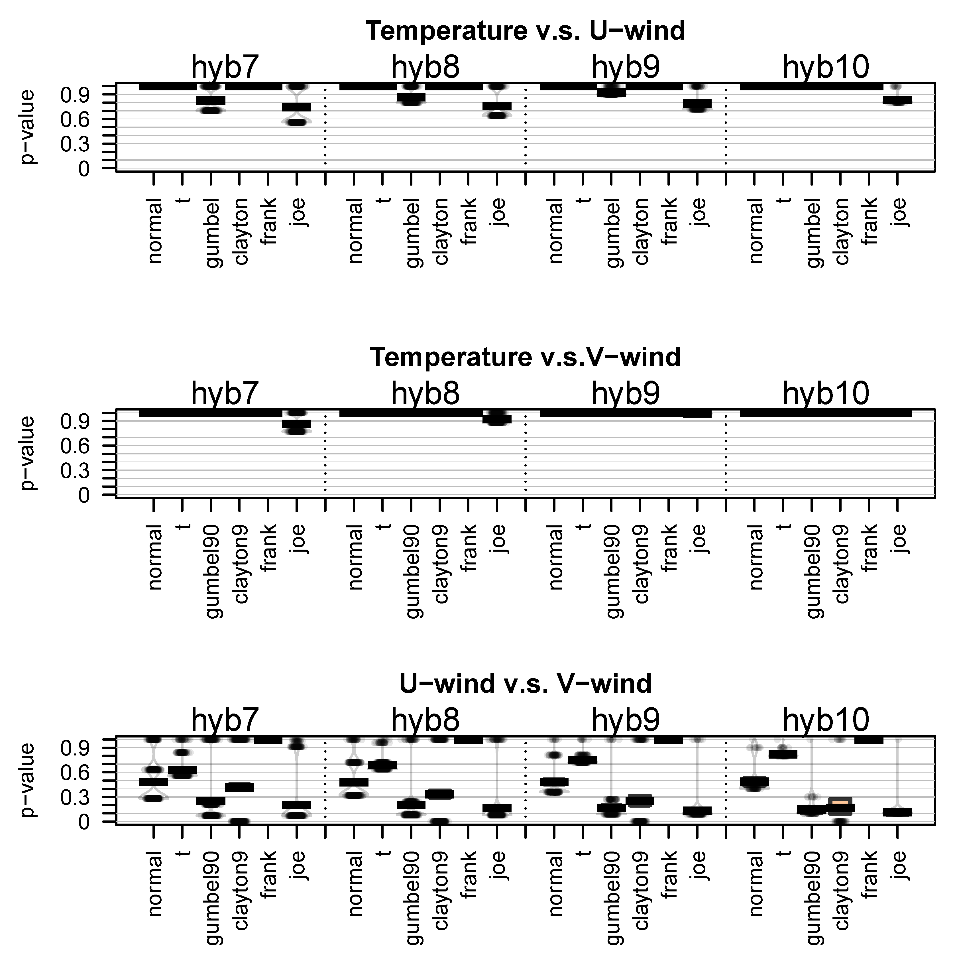
Figure 23 presents the pirateplots [53] of p-value results of hybrid tests of bivariates regarding Gaussian, t, Gumbel, Clayton, Frank, and Joe copula families. For the individual test, a parametric bootstrapping is performed to obtain numerous p-values, and the results of the hybrid tests include possible combinations of individual ones. The hybrid 7 in Figure 23 indicates a combination of seven different tests with q = 7 in (35). We consider 90-degrees rotated Gumbel and Clayton copulas due to the negative dependency between ( e Temp , e V - wind ) and ( e U - wind , e V - wind ) . Bivariate ( e Temp , e U - wind ) and ( e Temp , e V - wind ) accept almost all the copula families. The pair U-wind and V-wind fits better for Frank and t copula. In the final decision, we utilize the t copula for the joint distribution of errors by all three variables for its test values and feasibility to construct a multivariate copula.

4.3. Empirical Margins and Random Number Generator

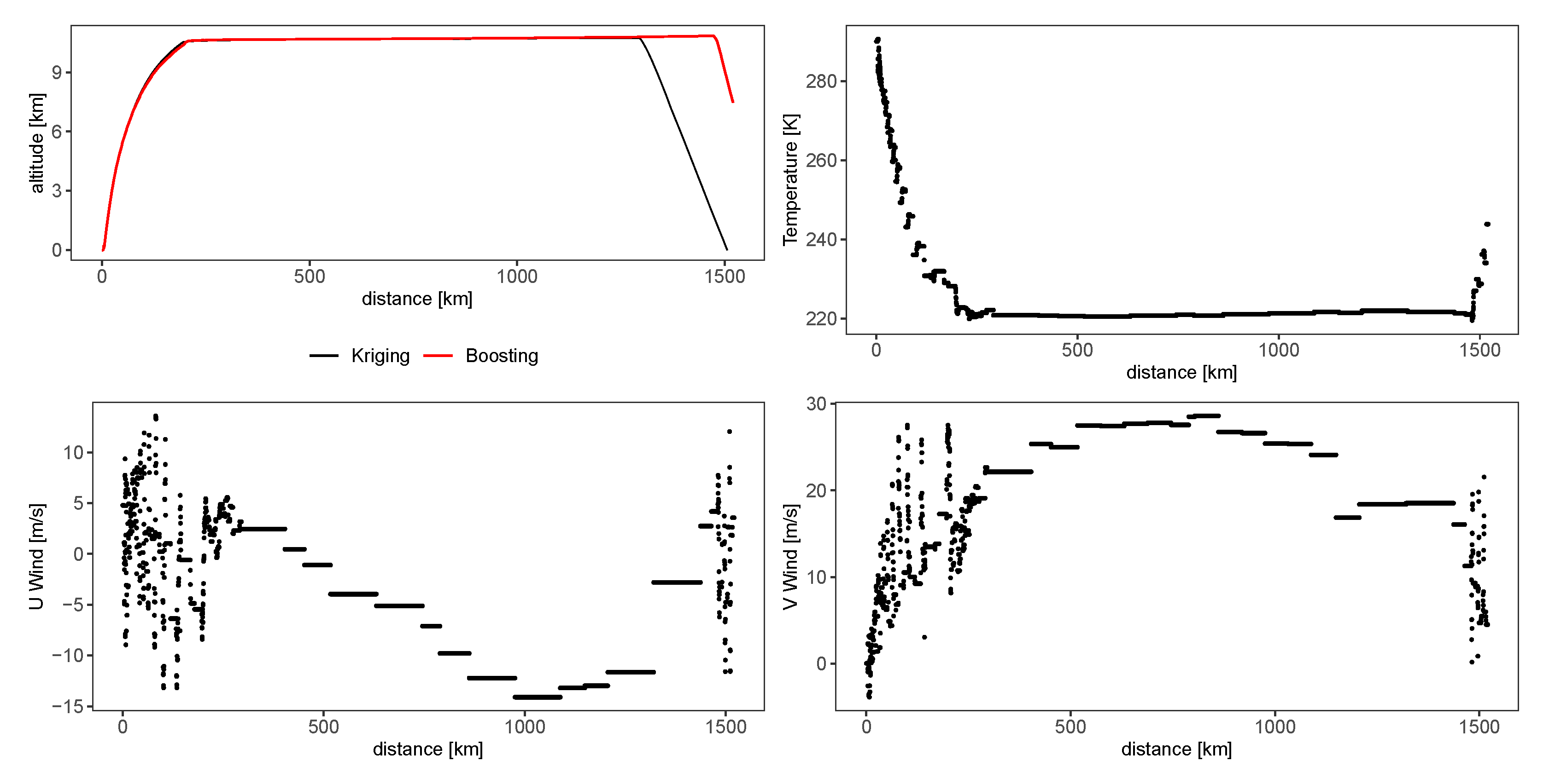
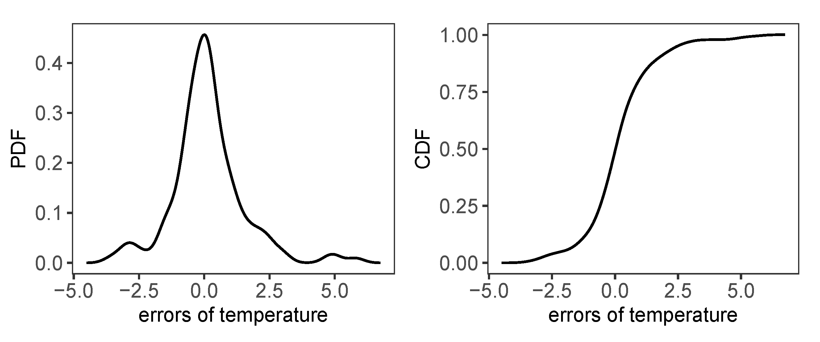
Simulation procedures are various for different copula families. The t copula is simulated using the normal mixture construction [45,54]. As for random number generation with the selected t copula, we first generate components ( u ˜ Temp , u ˜ U - wind , u ˜ V - wind ) C θ ^ t ; then generate the errors ( e ˜ Temp , e ˜ U - wind , e ˜ V - wind ) based on u ˜ with the inverse CDF method e ˜ j = F ˜ j 1 ( u ˜ j ) with j { Temp , U - wind , V - wind } , where F ˜ is a kernel-smoothed empirical cumulative distribution function, which together with the KDE are exemplarily for the temperature depicted in Figure 24. The simulated errors and the balloon-GFS errors have similar bivariate distributions, as can be seen from the contourplots Figure 25, where the simulated and balloon-GFS errors are in black and blue. This is exactly what we wanted to achieve in order to investigate the effect of error in the GFS data and the robustness of the SOPHIA. We then have the simulated weather scenarios by adding the simulated errors to GFS data, as in (32). There are n = 468 GFS grid points in our experiment from Prague to Tunis. The same number of distinct simulated errors are added to the GFS temperature, U-wind, and V-wind. The weather an aircraft experiences is interpolated by Kriging with the simulated errors added to the GFS data as an input, i.e., ( z ˜ Temp , z ˜ U - wind , z ˜ V - wind ) in (32). These weather values interpolated along the trajectory can be seen in Figure 26, where the black lines are the interpolated temperature, U-wind, and V-wind with the GFS data and the chromatic lines the interpolated value with simulated weather scenarios.

4.4. Trajectory Simulation Results

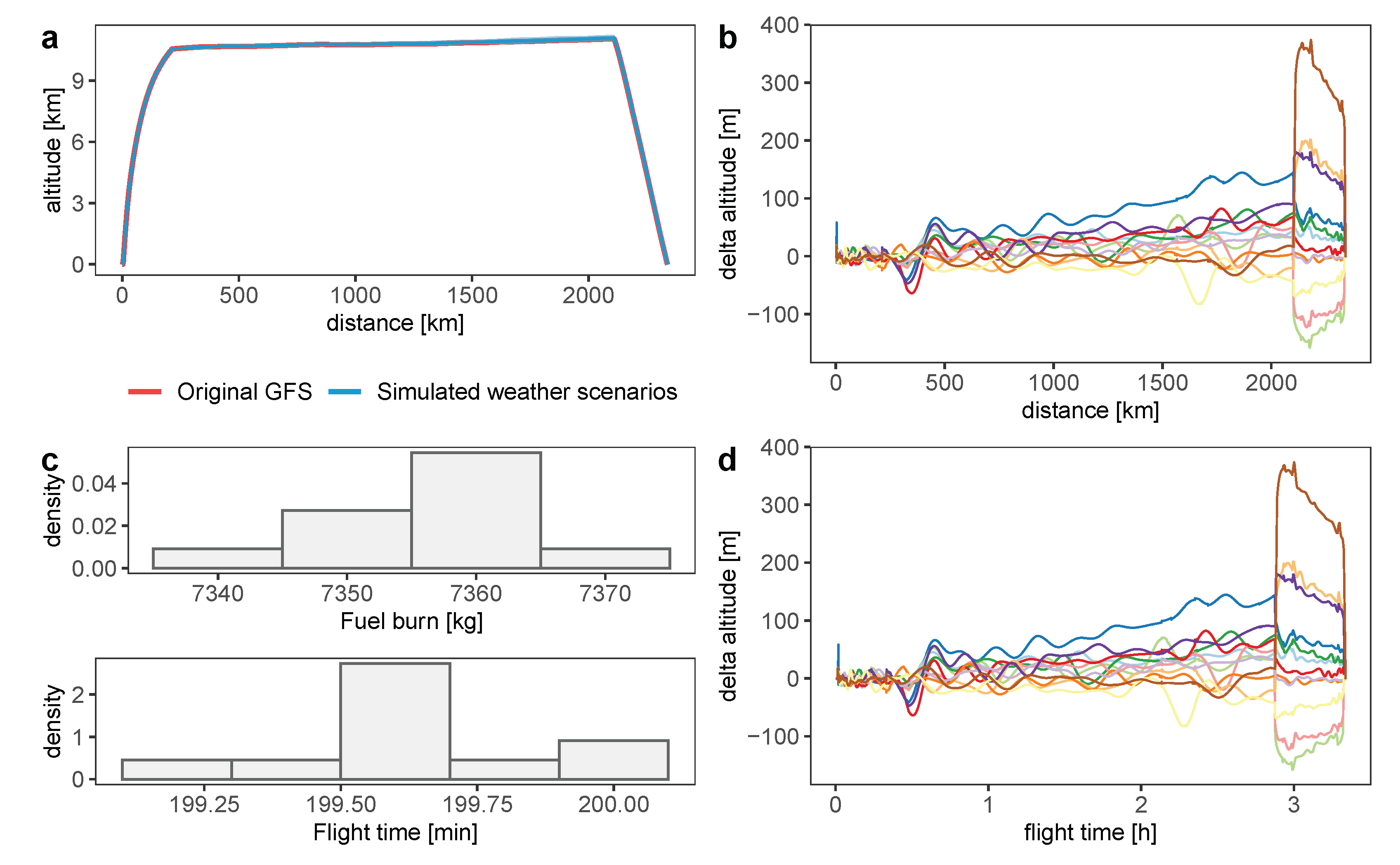
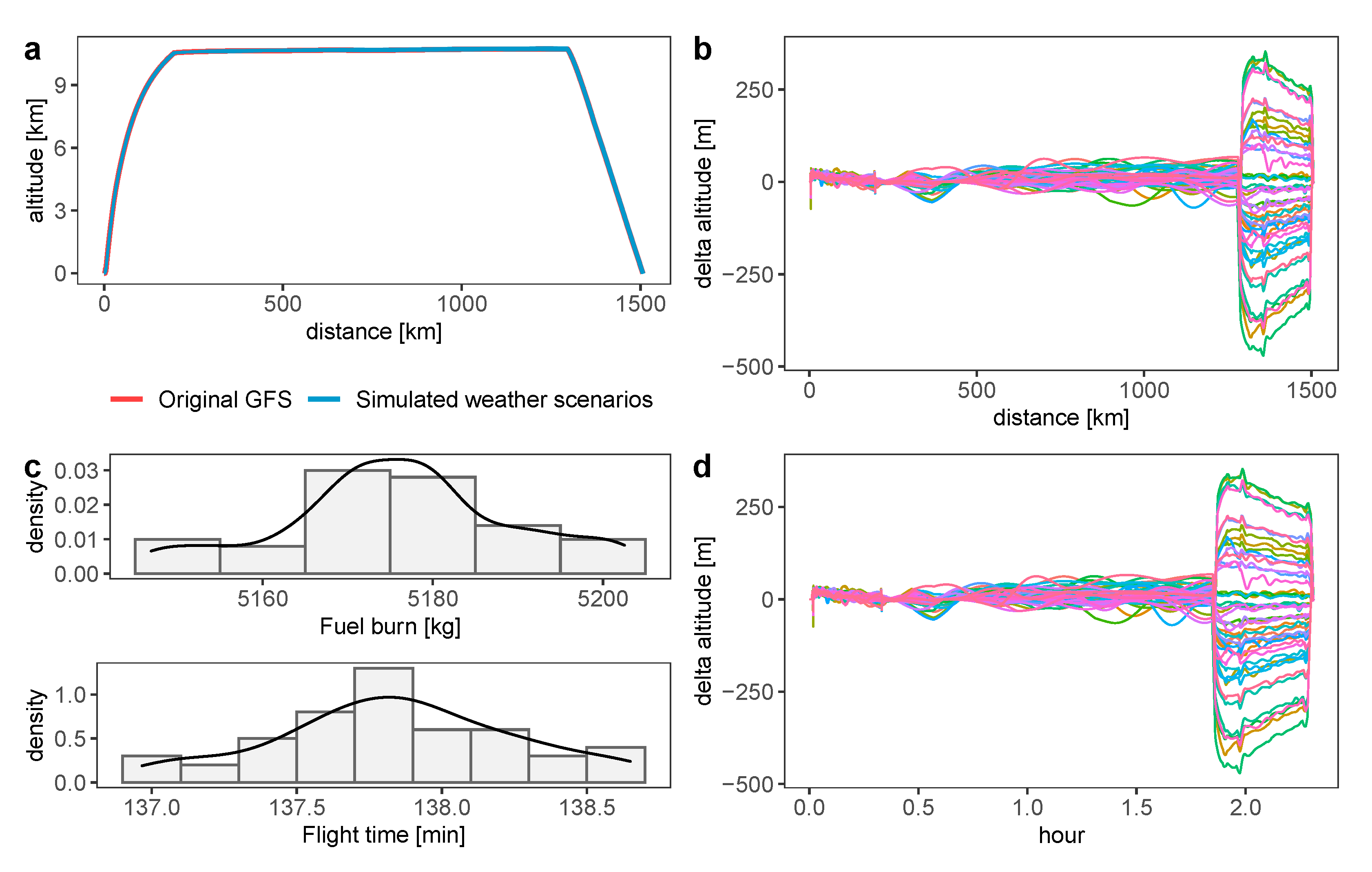
Given weather scenarios with GFS data and simulated errors, we can examine how the errors from GFS data and Kriging interpolation can impact the trajectories in SOPHIA. Figure 27a presents vertical profiles of 50 trajectories from Prague to Tunis, which have start, climb, cruise, and descent phases. The trivial difference can be spotted in the trajectories with the weather scenarios having the errors added. We use the trajectory with GFS inputs as the baseline to reveal such differences and calculate the altitude difference between the 50 trajectories with simulated weather scenarios and baseline trajectory in Figure 27b,d. The altitude differences in the start and climb phases are slight and increase as the travel distance increases in the cruise phase, resulting from cumulative differences along time. We can spot more visible differences during the descent phase because SOPHIA implements continuous descent operation (CDO) in search for the top of descent (TOD) to guarantee a maximum descent distance and minimum fuel burn [8]. Nevertheless, the differences are still within 300 m range. Besides the vertical profile, total fuel burn has variation within 70 kg and flight time in 3 min as in Figure 27c, which confirms the small impact of errors from GFS data and Kriging interpolation on the trajectories.

5. Conclusions

The atmospheric state has a significant impact on the motion of an aircraft and the optimized trajectories. The target function in the optimizer requires accurate meteorological data as input. In this paper, meteorological information such as temperature, wind speed, and wind direction can seriously influence the path and performance. We examined linear interpolation, RBF, Kriging, neural network, bagging, and GBM to interpolate weather variables for an accurate method. Linear interpolation, Ordinary Kriging, and the RBF method are accurate when evaluated by loo-MSE with GFS data from Prague to Tunis. Considering accuracy and time efficiency, we integrated Ordinary Kriging into SOPHIA. Nevertheless, errors in both GFS data and Ordinary Kriging are inevitable. This paper studies the impact of such inaccuracy, including in the GFS data and Kriging interpolation method, on the optimized trajectories. To achieve this, we further modelled the dependency of these variables with the copula and generated weather scenarios out of the copula model for SOPHIA as input. We simulated a trajectory from Prague to Tunis given the weather scenarios. Even though both GFS and Kriging are not accurate, these inaccuracies had a trivial impact on the trajectory, total fuel burn, and flight time, according to the simulation results. To summarize, we have confirmed that,
  • the kernel method works better than machine learning methods for the meteorological data interpolation for a flight trajectory;
  • even though errors in GFS data and Ordinary Kriging are inevitable, the inaccuracy of the data has a very minor impact on the trajectory, total fuel burn, and flight time.
Despite the fact that the trajectory simulation results from Prague to Tunis, and another trajectory from Nantes to Athens in the Appendix A, confirm the above statements, these two trajectories are restricted within the short trajectories in Europe. Other regions may not have weather balloon stations to provide data to compare with interpolation. Moreover, long-distance and cross-continent trajectories first require significant computational resources and can also overpass regions with no or scattered weather stations, making the GFS data unreliable and impractical to validate the effect of the inaccuracy of the data on the trajectory. This paper involves only the three-dimensional spatial interpolations, and the four-dimensional spatio-temporal interpolation still deserves further research. This four-dimensional spatio-temporal interpolation with the kernel methods also requires a fast implication for the trajectory optimizer.

Author Contributions

Conceptualization, O.O. and J.R.; methodology, O.O. and G.C.; software, O.O., G.C. and J.R.; validation, O.O. and H.F.; formal analysis, G.C.; investigation, G.C.; resources, O.O. and J.R.; data curation, G.C.; writing—original draft preparation, G.C., O.O. and J.R.; writing—review and editing, O.O., J.R. and H.F.; visualization, G.C.; supervision, O.O.; project administration, H.F. and J.R.; and funding acquisition, H.F. All authors have read and agreed to the published version of the manuscript.

Funding

This work is funded by the Deutsche Forschungsgemeinschaft (DFG, German Research Foundation) with Grant number FR 2440/7-1 in the framework of the project CDO-Speedbrakes.

Institutional Review Board Statement

Not applicable.

Informed Consent Statement

Not applicable.

Data Availability Statement

Publicly available datasets were analyzed in this study. The GFS data are openly available on https://www.ncei.noaa.gov/products/weather-climate-models/global-forecast (accessed on 31 August 2020); The weather balloon data can be found from the Integrated Global Radiosonde Archive (IGRA) https://www.ncei.noaa.gov/products/weather-balloon/integrated-global-radiosonde-archive (accessed on 18 December 2018).

Conflicts of Interest

The authors declare no conflict of interest. The funders had no role in the design of the study; in the collection, analyses, or interpretation of data; in the writing of the manuscript; or in the decision to publish the results.

Appendix A. A Trajectory from Nantes to Athens

Besides the trajectory from Prague to Tunis, we simulate another trajectory from Nantes to Athens to confirm that the errors in GFS data and Ordinary Kriging interpolation have a slight impact on the vertical profiles of the trajectory. Figure A1 presents the trajectory from Nantes to Athens; Figure A2a,b,d show vertical profiles and altitude differences with the simulated weather scenarios. The same pattern of cumulative differences along time can be seen as in Figure 27. The simulated weather scenarios produce small differences in fuel burn and flight time in Figure A2c.
Figure A1. Blue points: the GFS data; black points: weather stations; black curve: the trajectory from Nantes to Athens.
Stats 05 00018 g0a1
Figure A2. (a) The vertical profiles of the trajectories from Nantes to Athens by SOPHIA; red curve: with GFS data; blue curve: with simulated weather scenarios. (b,d) The chromatic line plots present the altitude differences between trajectories with simulated weather scenarios and GFS input. (c) Total fuel burn and flight time of 11 trajectories with simulated weather scenarios.
Stats 05 00018 g0a2

References

  1. Rosenow, J.; Fricke, H. Flight performance modeling to optimize trajectories. In Proceedings of the Deutscher Luft- und Raumfahrtkongress 2016, Braunschweig, Germany, 13–15 September 2016. [Google Scholar]
  2. Sun, J.; Hoekstra, J.M.; Ellerbroek, J. OpenAP: An Open-Source Aircraft Performance Model for Air Transportation Studies and Simulations. Aerospace 2020, 7, 104. [Google Scholar] [CrossRef]
  3. Krige, D.G. A statistical approach to some basic mine valuation problems on the Witwatersrand. J. S. Afr. Inst. Min. Metall. 1951, 52, 119–139. [Google Scholar]
  4. Johnson, J.E.; Laparra, V.; Pérez-Suay, A.; Mahecha, M.D.; Camps-Valls, G. Kernel methods and their derivatives: Concept and perspectives for the earth system sciences. PLoS ONE 2020, 15, e0235885. [Google Scholar] [CrossRef] [PubMed]
  5. Heryudono, A.R.H.; Driscoll, T.A. Radial Basis Function Interpolation on Irregular Domain through Conformal Transplantation. J. Sci. Comput. 2010, 44, 286–300. [Google Scholar] [CrossRef] [Green Version]
  6. Rosenow, J.; Lindner, M.; Scheiderer, J. Advanced Flight Planning and the Benefit of In-Flight Aircraft Trajectory Optimization. Sustainability 2021, 13, 1383. [Google Scholar] [CrossRef]
  7. Wynnyk, C.M. Wind analysis in aviation applications. In Proceedings of the 2012 IEEE/AIAA 31st Digital Avionics Systems Conference (DASC), Williamsburg, VA, USA, 14–18 October 2012; IEEE: Williamsburg, VA, USA, 2012; p. 5C2-1. [Google Scholar]
  8. Förster, S.; Rosenow, J.; Lindner, M.; Fricke, H. A Toolchain for Optimizing Trajectories under Real Weather Conditions and Realistic Flight Performance; Greener Aviation: Brussels, Belgium, 2016. [Google Scholar]
  9. Zhang, Y.; McGovern, S. Application of the Rapid Update Cycle (RUC) to Aircraft Flight Simulation. In Volume 14: New Developments in Simulation Methods and Software for Engineering Applications, ASME International Mechanical Engineering Congress and Exposition; ASME: New York, NY, USA, 2008; pp. 45–53. [Google Scholar] [CrossRef] [Green Version]
  10. Félix Patrón, R.S.; Botez, R.M. Flight Trajectory Optimization Through Genetic Algorithms Coupling Vertical and Lateral Profiles. In Volume 1: Advances in Aerospace Technology, ASME International Mechanical Engineering Congress and Exposition; ASME: New York, NY, USA, 2014; p. V001T01A048. [Google Scholar] [CrossRef]
  11. Olivares, A.; Soler, M.; Staffetti, E. Multiphase mixed-integer optimal control applied to 4D trajectory planning in air traffic management. In Proceedings of the 3rd International Conference on Application and Theory of Automation in Command and Control Systems, Napoli, Italy, 28–30 May 2013; pp. 85–94. [Google Scholar]
  12. Friedland, C.J.; Joyner, T.A.; Massarra, C.; Rohli, R.V.; Treviño, A.M.; Ghosh, S.; Huyck, C.; Weatherhead, M. Isotropic and anisotropic kriging approaches for interpolating surface-level wind speeds across large, geographically diverse regions. Geomat. Nat. Hazards Risk 2017, 8, 207–224. [Google Scholar] [CrossRef]
  13. Zhu, A.X.; Lu, G.; Liu, J.; Qin, C.Z.; Zhou, C. Spatial prediction based on Third Law of Geography. Ann. GIS 2018, 24, 225–240. [Google Scholar] [CrossRef]
  14. Wong, D.W.; Yuan, L.; Perlin, S.A. Comparison of spatial interpolation methods for the estimation of air quality data. J. Expos. Sci. Environ. Epidemiol. 2004, 14, 404–415. [Google Scholar] [CrossRef] [Green Version]
  15. Heddam, S.; Keshtegar, B.; Kisi, O. Predicting total dissolved gas concentration on a daily scale using kriging interpolation, response surface method and artificial neural network: Case study of Columbia river Basin Dams, USA. Nat. Resour. Res. 2020, 29, 1801–1818. [Google Scholar] [CrossRef]
  16. Rigol, J.P.; Jarvis, C.H.; Stuart, N. Artificial neural networks as a tool for spatial interpolation. Int. J. Geogr. Inf. Sci. 2001, 15, 323–343. [Google Scholar] [CrossRef]
  17. Li, J.; Heap, A.D.; Potter, A.; Daniell, J.J. Application of machine learning methods to spatial interpolation of environmental variables. Environ. Model. Softw. 2011, 26, 1647–1659. [Google Scholar] [CrossRef]
  18. Li, J.; Siwabessy, J.; Huang, Z.; Nichol, S. Developing an Optimal Spatial Predictive Model for Seabed Sand Content Using Machine Learning, Geostatistics, and Their Hybrid Methods. Geosciences 2019, 9, 180. [Google Scholar] [CrossRef] [Green Version]
  19. Trüb, R.; Moser, D.; Schäfer, M.; Pinheiro, R.; Lenders, V. Monitoring meteorological parameters with crowdsourced air traffic control data. In Proceedings of the 2018 17th ACM/IEEE International Conference on Information Processing in Sensor Networks (IPSN), Porto, Portugal, 11–13 April 2018; IEEE: Piscataway, NJ, USA, 2018; pp. 25–36. [Google Scholar]
  20. Stone, E.K.; Kitchen, M. Introducing an approach for extracting temperature from aircraft GNSS and pressure altitude reports in ADS-B messages. J. Atmos. Ocean. Technol. 2015, 32, 736–743. [Google Scholar] [CrossRef]
  21. Murrieta-Mendoza, A.; Romain, C.; Botez, R.M. 3D Cruise trajectory optimization inspired by a shortest path algorithm. Aerospace 2020, 7, 99. [Google Scholar] [CrossRef]
  22. Cressie, N.; Wikle, C.K. Statistics for Spatio-Temporal Data; John Wiley & Sons: New York, NY, USA, 2015. [Google Scholar]
  23. Gratton, G. Initial Airworthiness; Springer: Berlin, Germany, 2016. [Google Scholar]
  24. Dalmau, R.; Pérez-Batlle, M.; Prats, X. Estimation and prediction of weather variables from surveillance data using spatio-temporal Kriging. In Proceedings of the 2017 IEEE/AIAA 36th Digital Avionics Systems Conference (DASC), St. Petersburg, FL, USA, 17–21 September 2017; IEEE: Piscataway, NJ, USA, 2017; pp. 1–8. [Google Scholar]
  25. Esmaeilbeigi, M.; Chatrabgoun, O. An efficient method based on RBFs for multilayer data interpolation with application in air pollution data analysis. Comput. Appl. Math. 2019, 38, 1–20. [Google Scholar] [CrossRef]
  26. Fasshauer, G.; McCourt, M. Kernel-Based Approximation Methods Using MATLAB; World Scientific Publishing Company: London, UK, 2015; Volume 19. [Google Scholar]
  27. Nash, J.C.; Varadhan, R. Unifying Optimization Algorithms to Aid Software System Users: Optimx for R. J. Stat. Softw. 2011, 43, 1–14. [Google Scholar] [CrossRef] [Green Version]
  28. Montero, J.M.; Fernández-Avilés, G.; Mateu, J. Spatial and Spatio-Temporal Geostatistical Modeling and Kriging; John Wiley & Sons: New York, NY, USA, 2015; Volume 998. [Google Scholar]
  29. Pebesma, E.J. Multivariable geostatistics in S: The gstat package. Comput. Geosci. 2004, 30, 683–691. [Google Scholar] [CrossRef]
  30. Perperoglou, A.; Sauerbrei, W.; Abrahamowicz, M.; Schmid, M. A review of spline function procedures in R. BMC Med. Res. Methodol. 2019, 19, 46. [Google Scholar] [CrossRef] [Green Version]
  31. Goodfellow, I.; Bengio, Y.; Courville, A. Deep Learning; MIT Press: Cambridge, MA, USA, 2016. [Google Scholar]
  32. Efron, B.; Hastie, T. Computer Age Statistical Inference; Cambridge University Press: Cambridge, UK, 2016; Volume 5. [Google Scholar]
  33. Abadi, M.; Agarwal, A.; Barham, P.; Brevdo, E.; Chen, Z.; Citro, C.; Corrado, G.S.; Davis, A.; Dean, J.; Devin, M.; et al. TensorFlow: Large-Scale Machine Learning on Heterogeneous Systems, 2015. Software. Available online: https://tensorflow.org (accessed on 3 March 2020).
  34. Chollet, F. Keras. 2015. Available online: https://github.com/fchollet/keras (accessed on 3 March 2020).
  35. Hastie, T.; Tibshirani, R.; Friedman, J. The Elements of Statistical Learning: Data Mining, Inference, and Prediction; Springer: Berlin, Germany, 2009. [Google Scholar]
  36. Friedman, J.H. Greedy function approximation: A gradient boosting machine. Ann. Stat. 2001, 29, 1189–1232. [Google Scholar] [CrossRef]
  37. Boehmke, B.; Greenwell, B.M. Hands-on Machine Learning with R; CRC Press: Boca Raton, FL, USA, 2019. [Google Scholar]
  38. Chen, T.; Guestrin, C. XGBoost: A Scalable Tree Boosting System. In Proceedings of the KDD ’16, 22nd ACM SIGKDD International Conference on Knowledge Discovery and Data Mining, San Francisco, CA, USA, 13–17 August 2016; ACM: New York, NY, USA, 2016; pp. 785–794. [Google Scholar] [CrossRef] [Green Version]
  39. Hollander, M.; Wolfe, D.A.; Chicken, E. Nonparametric Statistical Methods; John Wiley & Sons: New York, NY, USA, 2013; Volume 751. [Google Scholar]
  40. Möller, A.; Lenkoski, A.; Thorarinsdottir, T.L. Multivariate probabilistic forecasting using ensemble Bayesian model averaging and copulas. Q. J. R. Meteorol. Soc. 2013, 139, 982–991. [Google Scholar] [CrossRef] [Green Version]
  41. Lazoglou, G.; Anagnostopoulou, C. Joint distribution of temperature and precipitation in the Mediterranean, using the Copula method. Theor. Appl. Climatol. 2019, 135, 1399–1411. [Google Scholar] [CrossRef]
  42. Sklar, M. Fonctions de repartition an dimensions et leurs marges. Publ. Inst. Stat. Univ. Paris 1959, 8, 229–231. [Google Scholar]
  43. Größer, J.; Okhrin, O. Copulae: An overview and recent developments. In Wiley Interdisciplinary Reviews: Computational Statistics; Wiley Online Library: New York, NY, USA, 2021; p. e1557. [Google Scholar]
  44. Nelsen, R.B. An Introduction to Copulas; Springer: Berlin, Germany, 2007. [Google Scholar]
  45. Hofert, M.; Kojadinovic, I.; Mächler, M.; Yan, J. Elements of Copula Modeling with R; Springer: Berlin, Germany, 2019. [Google Scholar]
  46. Zhang, S.; Okhrin, O.; Zhou, Q.M.; Song, P.X.K. Goodness-of-fit test for specification of semiparametric copula dependence models. J. Econ. 2016, 193, 215–233. [Google Scholar] [CrossRef] [Green Version]
  47. Genest, C.; Rémillard, B.; Beaudoin, D. Goodness-of-fit tests for copulas: A review and a power study. Insur. Math. Econ. 2009, 44, 199–213. [Google Scholar] [CrossRef]
  48. Okhrin, O.; Trimborn, S.; Waltz, M. gofCopula: Goodness-of-Fit tests for copulae. R J. 2021, 13, 467–498. [Google Scholar] [CrossRef]
  49. Huang, W.; Prokhorov, A. A goodness-of-fit test for copulas. Econ. Rev. 2014, 33, 751–771. [Google Scholar] [CrossRef] [Green Version]
  50. Genest, C.; Quessy, J.F.; Rémillard, B. Goodness-of-fit procedures for copula models based on the probability integral transformation. Scand. J. Stat. 2006, 33, 337–366. [Google Scholar] [CrossRef]
  51. Breymann, W.; Dias, A.; Embrechts, P. Dependence structures for multivariate high-frequency data in finance. Quant. Financ. 2003, 3, 1–14. [Google Scholar] [CrossRef]
  52. Scaillet, O. Kernel-based goodness-of-fit tests for copulas with fixed smoothing parameters. J. Multivar. Anal. 2007, 98, 533–543. [Google Scholar] [CrossRef]
  53. Phillips, N. Yarrr: A Companion to the E-Book “Yarrr!: The Pirate’s Guide to R”. Computer Software Manual]. R Package Version 0.1. 5. 2017. Available online: https:/CRAN.R-project.org/package=yarrr (accessed on 7 January 2019).
  54. Demarta, S.; McNeil, A.J. The t copula and related copulas. Int. Stat. Rev. 2005, 73, 111–129. [Google Scholar] [CrossRef]
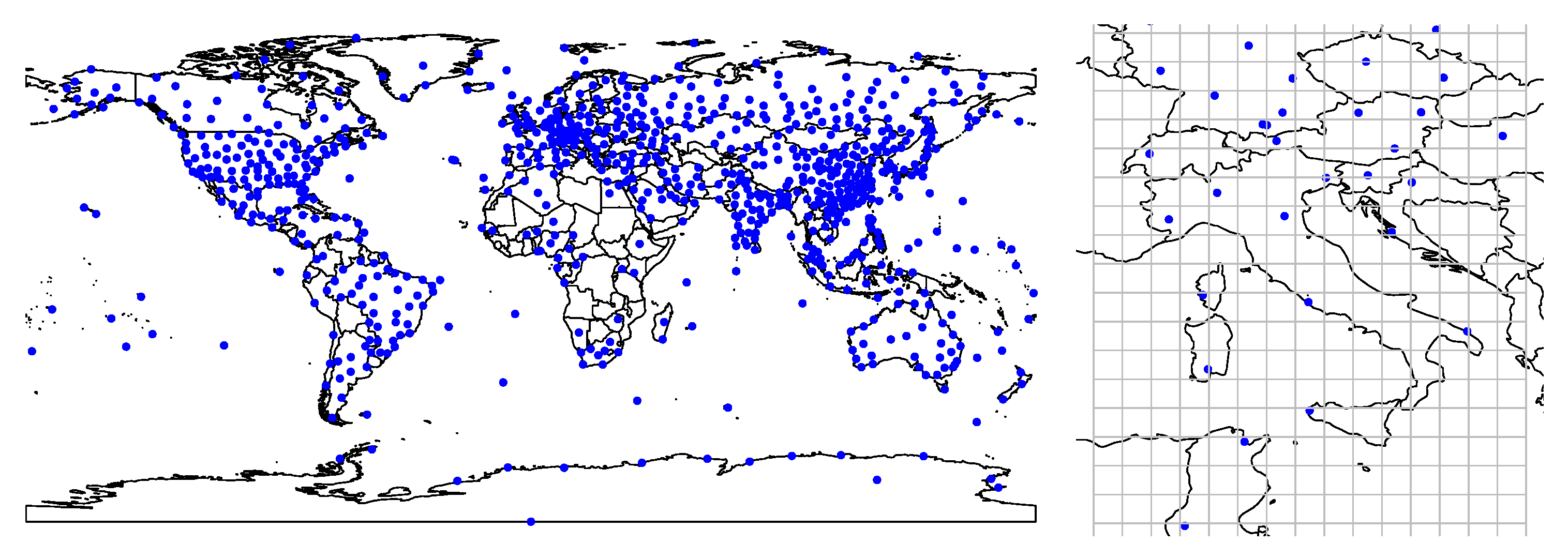
Figure 1. (Left) Locations of 813 weather balloon stations. (Right) A comparison of weather balloon stations collaborating with NCEP in Europe and GFS data grid (crossings of the gray grid with one-degree resolution). Data are from www.ncdc.noaa.gov (accessed on 13 November 2018).
Stats 05 00018 g001
Figure 2. A snapshot of temperature (in Kelvin) with GFS data on 4th of September 2018 and longitude ranges from 15E to 20E, latitude from 35N to 40N.
Stats 05 00018 g002
Figure 3. Wind vector Z w and components U-wind and V-wind.
Stats 05 00018 g003
Figure 4. Boxplots of three variables grouped by air pressure with a snapshot on 4th of September 2018 and longitude ranges from 15E to 20E, latitude from 35N to 40N.
Stats 05 00018 g004
Figure 5. Points: weather data from GFS; curve: fitted non-linear regression.
Stats 05 00018 g005
Figure 6. The blue points denote the GFS data used along the trajectory (black curve) from Prague to Tunis.
Stats 05 00018 g006
Figure 7. A simplication to estimate z ( s 0 ) based on z ( s i ) and z ( s j ) with linear interpolation for d = 1 .
Stats 05 00018 g007
Figure 8. A representation to estimate dimension by dimension with linear interpolation for d = 3 . s 1 , s 2 , , s 8 are the observations, and s 0 lies on the grey plane. The value at the intermediate locations ( s 9 , s 10 , s 11 , s 12 ) and ( s 13 , s 14 ) are to be interpolated.
Stats 05 00018 g008
Figure 9. LOOCV for linear interpolation with six nearest observations.
Stats 05 00018 g009
Figure 10. The RBF method interpolation surface with ε = ( 0.01 , 1 , 10 ) . When ε = 0.01 , interpolation surface is flat (left), ε = 1 returns a satisfactory surface (middle), when ε = 10 , surface will be noisy (right).
Stats 05 00018 g010
Figure 11. Semivariance γ ^ ( h ) = 7.38 4.15 e h / 9.46 and Covariance C ( h ) = 4.15 e h / 9.46 when h > 0 .
Stats 05 00018 g011
Figure 12. (Left) Scatterplot of temperature and three trend models: spline, linear regression, and ISA. (Right) LOOCV errors with four trend models.
Stats 05 00018 g012
Figure 13. In-sample interpolation of wind speed with Ordinary Kriging demonstrates the necessity of the scaling factor. Data are from GFS analysis data on 3 November 2018, with longitude ranges from 5E to 10E and latitude from 45N to 50N.
Stats 05 00018 g013
Figure 14. The scaling function for the altitude. Blue points: target GFS altitude and scaling results; black curve: the scaling function (22).
Stats 05 00018 g014
Figure 15. (Left) the original GFS data with various gaps along the altitude; (Right) rescaled altitude of the vertical dimension with (22).
Stats 05 00018 g015
Figure 16. Curves: semivariance models γ ^ ( h ) for temperature, wind speed, and relative humidity; points: empirical semivariance γ ^ z ( h ) calculated by (19).
Stats 05 00018 g016
Figure 17. cv-MSE and epochs with five neural network models for temperature, wind speed, and relative humidity. Sizes of networks grow from a small model with one hidden layer to a huge model with four hidden layers. Validation errors and training errors are denoted with dashed and solid lines, respectively.
Stats 05 00018 g017
Figure 18. Ten-fold cross-validation RMSE by iteration using GBM. Train and validation sets are distinguished by solid and dashed lines.
Stats 05 00018 g018
Figure 19. Trajectory generated by SOPHIA (topleft) and weather information interpolated by GBM.
Stats 05 00018 g019
Figure 20. Blue points: the GFS data; black points: weather stations; black curve: the trajectory from Prague to Tunis.
Stats 05 00018 g020
Figure 21. The pirateplots of the errors of three timestamps interpolated using Kriging with the GFS data as input evaluated by the balloons data.
Stats 05 00018 g021
Figure 22. Normal scores of the errors between weather variables.
Stats 05 00018 g022
Figure 23. Hybrid Goodness-of-fit p values of the Gaussian, t, Gumbel, Clayton, Frank, and Joe copula families. A p-value close to zero will reject the copula family hypothesis.
Stats 05 00018 g023
Figure 24. Kernel smoothed empirical PDF (left) and CDF (right) of errors of temperature by the difference of balloon data and estimates by Kriging.
Stats 05 00018 g024
Figure 25. Contourplots of the errors from the difference of balloon data and interpolated values with GFS data and simulated errors generated by t copula and kernel-smoothed empirical CDF.
Stats 05 00018 g025
Figure 26. The black curve: the interpolation value with the GFS data; the chromatic curves: the interpolated values with simulated weather scenarios.
Stats 05 00018 g026
Figure 27. (a) The vertical profiles of the trajectories from Prague to Tunis by SOPHIA; red curve: with GFS data; blue curve: with simulated weather scenarios. (b,d) The chromatic line plots present the altitude differences between trajectories with simulated weather scenarios and GFS input. (c) Total fuel burn and flight time of 50 trajectories with simulated weather scenarios.
Stats 05 00018 g027
Table 1. cv-MSE on the test set with four network models of different sizes.
Model SizeUnitsActivationcv-MSE 1
Temperature (K2)Wind Speed ( m 2 · s 2 )Relative Humidity (%2)
Hidden layersSmall50tanh652.7078.07599.68
Medium300tanh652.8033.54582.77
50tanh
Large400tanh17.0534.83581.41
100tanh
50linear
Huge500tanh7.1633.16424.28
300tanh
100tanh
50linear
1 cv-MSE results are averaged over the last 20 epochs.
Table 2. cv-MSE cross-validation results with grid search for parameter α in the regularized neural network.
α00.0010.010.11101001000
Temperature (K 2 )9.846.037.2811.0718.599.5029.46536.56
Wind speed ( m 2 · s 2 )38.8439.3639.5840.5039.0641.1677.5577.69
Relative humidity (% 2 )593.05585.94559.01536.48481.06600.70654.94652.03
Table 3. loo-MSE for methods with GFS data along the trajectory from Prague to Tunis.
Methodsloo-MSE
Temperature (K2)Wind Speed ( m 2 · s 2 )Relative Humidity (%2)
Ordinary Kriging11.793.5369.10
the RBF method0.421.9385.73
Neural Network13.0547.33678.50
Bagging15.0416.15153.29
GBM2.3913.34179.21
Linear Interpolation9.3113.01178.11
Table 4. Dependency test of the errors between weather variables.
ρ s p ρ τ p τ
Temperature (K)U-wind (m/s)0.120.190.080.08 (positive)
Temperature (K)V-wind (m/s)−0.190.04−0.120.02 (negative)
U-wind (m/s)V-wind (m/s)−0.130.16−0.100.06 (negative)
Table 5. Archimedean copula families with one-parameter generator functions ϕ used in this paper.
Family θ ϕ ( t ) C ( u 1 , u 2 )
Gumbel θ [ 1 , ) exp ( t ) exp ( log u 1 ) θ + ( log u 2 ) θ 1 / θ  
Clayton θ [ 1 , ) 1 θ max ( u 1 θ + u 2 θ 1 , 0 1 / θ  
Frank θ ( , ) \ { 0 } log exp ( θ t ) 1 exp ( θ ) 1 1 θ log 1 + ( exp ( θ u 1 ) 1 ) ( exp ( θ u 2 ) 1 ) exp ( θ ) 1  
Joe θ [ 1 , ) log { 1 ( 1 t ) θ } 1 ( 1 u 1 ) θ + ( 1 u 2 ) θ ( 1 u 1 ) θ ( 1 u 2 ) θ 1 / θ
Publisher’s Note: MDPI stays neutral with regard to jurisdictional claims in published maps and institutional affiliations.