Analysis of Household Pulse Survey Public-Use Microdata via Unit-Level Models for Informative Sampling

Abstract

The Household Pulse Survey, recently released by the U.S. Census Bureau, gathers information about the respondents’ experiences regarding employment status, food security, housing, physical and mental health, access to health care, and education disruption. Design-based estimates are produced for all 50 states and the District of Columbia (DC), as well as 15 Metropolitan Statistical Areas (MSAs). Using public-use microdata, this paper explores the effectiveness of using unit-level model-based estimators that incorporate spatial dependence for the Household Pulse Survey. In particular, we consider Bayesian hierarchical model-based spatial estimates for both a binomial and a multinomial response under informative sampling. Importantly, we demonstrate that these models can be easily estimated using Hamiltonian Monte Carlo through the Stan software package. In doing so, these models can readily be implemented in a production environment. For both the binomial and multinomial responses, an empirical simulation study is conducted, which compares spatial and non-spatial models. Finally, using public-use Household Pulse Survey micro-data, we provide an analysis that compares both design-based and model-based estimators and demonstrates a reduction in standard errors for the model-based approaches.

1. Introduction

In recent years, COVID-19 has spread across the globe, causing immeasurable disruption in nearly every country. Governments and policy-makers around the world have been forced to institute a range of public heath and social measures, from movement restrictions to the closure of schools and businesses. In the United States, many impactful measures have been taken at the state or local level, such as mask mandates, testing, and contact tracing protocols. Furthermore, the societal effects of COVID-19 may differ across states for reasons such as population density, economic conditions, and demographic composition. According to the CDC [1], Black and Latino Americans are four times more likely to be hospitalized in comparison to non-Hispanic Whites, resulting in lost wages and healthcare expenses and deepening the racial wealth gap. To study this impact, the U.S. Census Bureau, in collaboration with multiple federal agencies, commissioned the Household Pulse Survey [2]. Other efforts to measure the societal effects of COVID-19 include the Research and Development Survey (RANDS) administered by the National Center for Health Statistics (NCHS). RANDS focuses on healthcare, such as telemedicine and access, as well as loss of work due to illness [3].

These surveys can better inform the American public as well as lawmakers, not only regarding the efficacy of the U.S. pandemic response but also the effects of stimulus measures that were enacted in order to sustain the economy. To address COVID-19, Congress has passed the CARES Act. Due to the frequent and timely dissemination of tabulations from the Household Pulse Survey, this survey may be a suitable tool to evaluate the efficacy of CARES and the demand for follow-up legislation. The Household Pulse Survey should inform law and policy-makers as to the magnitude of intervention necessary to secure Americans’ health and financial well-being. Additionally, the 116th U.S. Congress passed the Consolidated Appropriations Acts [4], which included $900 billion for COVID-19 relief; top ticket items included $325 billion for small businesses, $166 billion for stimulus checks, and $120 billion for increased federal unemployment benefits. With the inauguration of the 117th U.S. Congress, the $1.9 trillion American Rescue Plan [5] was also passed.

Historically, small-area estimation (SAE) techniques have been used in conjunction with survey data in order to provide population estimates for domains with small sample sizes [6]. There is a considerable literature on area-level models, such as the foundational Fay–Herriot model [7]. However, recently, there has been an increased demand for unit-level models that act on the survey data directly. For example, the basic unit-level model, or nested-error regression model [8] links individual survey units to geographic domains. This model can easily be fit using the sae package in R [9]. The choice of whether to model at the unit- or area-level is often the result of practical considerations, e.g., data availability. From a data-user perspective, area-level models may be necessary, as access to microdata (often confidential) may not be possible at the level of granularity desired for a specific analysis. From the perspective of an official statistical agency, this barrier may not be present. See [10] for additional discussion.

Unit-level models can offer greater precision as well as other benefits, such as a reduced reliance on ad-hoc benchmarking techniques; however, these come with their own set of challenges. First, it is critical to account for sample design in unit-level modeling, in order to mitigate biases [11]. The authors of [12] review many of the modern methods for accounting for an informative sampling design. One common approach is the use of a survey weighted pseudo-likelihood [13,14]. For example, [15] uses a pseudo-likelihood in conjunction with poststratification in order to estimate the prevalence of Chronic Obstructive Pulmonary Disease (COPD). Another approach to the informative sampling problem is the use of nonlinear regression techniques on the survey weights [16,17]; however, this approach can be quite computationally expensive and does not naturally incorporate covariates.

A second concern when using unit-level models is that they are often much more computationally demanding than their area-level counterparts. This is driven by increasingly large datasets at the unit level, as well as the prevalence of non-Gaussian data types. The authors of [18] use conjugate distribution theory to efficiently model Poisson data under a pseudo-likelihood, whereas [19] explore the use of data augmentation and a variational Bayes algorithm for binary and categorical data types under a pseudo-likelihood.

Within SAE, a specification of spatial dependence structure is often used to improve the precision of estimates. For example, at the area level, [20] consider conditional autoregressive priors on the area-level random effects, whereas [21] use Moran’s I basis functions. At the unit level, [17] use intrinsic conditional autoregressive (ICAR) priors in conjunction with a nonlinear regression on the survey weights. Alternatively, [19] use spatial Basis functions combined with a pseudo-likelihood.

In this work, rather than relying on custom sampling and estimation techniques, we demonstrate that openly available software can often be adequate for unit-level SAE. In particular, we develop a set of both spatial and non-spatial models for both binary and categorical survey data, within the popular probabilistic programming language, Stan [22]. Our model development is most similar in structure to that of [19], although we note that we use ICAR prior distributions for the spatial random effects and estimate the model automatically via Stan, rather than relying on custom sampling techniques. The primary contribution of this work is in the application of these methods to an important and timely dataset. In particular, as a motivating application, we construct state level estimates using the Household Pulse Survey, in order to better understand the societal effects of COVID-19 in the United States.

1.1. Household Pulse Survey

The Household Pulse Survey (HPS) gathers individual information about the respondents experiences regarding employment status, food security, housing, physical and mental health, access to health care, and education disruption [23]. Estimates are produced for all 50 states plus the District of Columbia (DC), as well as 15 Metropolitan Statistical Areas (MSAs), for a total of 66 areas. The survey is designed to provide timely and accurate weekly estimates. Samples are drawn from the Census Bureau’s Master Address File in combination with the Census Bureau Contact Frame and contacted via email and text. Once a household has completed the interview, their response remains in the sample for two weeks. Sample sizes were constructed appropriately to detect a two-percentage-point difference in weekly estimates, with an anticipated response rate of five percent. Sample sizes averaged around 1778 units per state per week, with a median of 1555, but ranged from as high as 9661 for California in Week 3 to as low as 360 for North Dakota in Week 2.

Sampling rates for each county are determined at the state level. Counties that belong in an MSA would require a larger sample to satisfy MSA sampling requirements. For example, the MSA counties within Maryland would require larger samples compared to the remaining counties within the state. These sampling rates inform a set of base weights. Sampling base weights in each of the 66 sample areas are calculated as the total number of eligible housing units (HU) divided by the number of HUs selected to be in the survey each week. In other words, the base weights of the sampled HUs sum to the total number of HUs.

Base weights are then adjusted to account nonresponse, the number of adults per household, and coverage. The base weights underwent four adjustments. (1) Non-response adjustment: the weight of those that did not respond were allocated to those that did respond for the same week and sample area. (2) Occupied HU ratio adjustment: HU weights were inflated to account for undercoverage in the sampling frame by matching weights post non-response adjustment to independent controls for the number of occupied HUs within each state according to the 2018 American Community Survey (ACS) one-year, state-level estimates. (3) Person adjustment converts HU weights into person weights by considering the number of adults aged 18 and over living within a given household. (4) Iterative Raking Ratio to Population Estimates: this weight adjustment uses the demographics of our sample to match education attainment estimates by age and sex of the 2018 1-year ACS estimates and the 2020 Hispanic origin/race by age and sex of the Census Bureau’s Population Estimates Program (PEP) for each state or MSA [23].

The Household Pulse Survey is split into phases, and is currently in Phase 3.3. Phase 1 began on 23 April 2020 and ended on 21 July 2020. Phase 2 began on 19 August 2020 and ended on 26 October 2020. Phase 3 began on 28 October 2020 and is ongoing. The Household Pulse Survey is released weekly and estimates (both point estimates and associated standard errors) are tabulated using the design-based Horvitz-Thompson estimator. Geographies include United States, 50 states plus DC, and 15 MAS, and estimates are further broken down by age, race, sex, education, etc. However, no cross-tabulations (for example age by sex) are available.

The remainder of this article is organized as follows. In Section 2 we present a series of unit-level models for binary and categorical survey data. Section 3 considers an empirical simulation study that utilizes the HPS. In Section 4, we illustrate our methodology by constructing state-level estimates with the HPS. Finally, in Section 5, we provide a discussion and concluding remarks. The Stan code files used to develop the simulations and data analysis are openly available at https://github.com/QuarkofDorothy/Analysis-of-HPS-Public-Use-Microdata-via-Unit-Level-Models-for-Informative-Sampling.git (accessed on 4 January 2022).

2. Methodology

2.1. Design-Based Estimation

Design-based approaches to estimation are interested in quantitative characteristics of a finite population. Inference is made based on the characteristics of repeated sampling from a population. Each unit in the population, $\mathcal{U}=\left\{1,\dots ,N\right\},$ has a probability of sample selection, ${\pi }_i$. We denote $w_i$ as the unit sample weight, typically assumed to be the inverse probability of selection. In the case of the HPS, these weights are adjusted as described in Section 1.1. The sample of size n is then denoted as $\mathcal{S}=\left\{1,\dots ,n\right\}$. Then, using complex survey methods for the sample data, we can derive an estimate for a given population quantity [24].

The HPS uses the Horvitz–Thompson estimator [25] for various population totals,

$$\begin{array}{c}\hfill {\widehat{t}}_{HT}=\sum _{i=1}^n{w}_i{y}_i,\end{array}$$

where $y_i$ is the response of interest for unit i in the sample. The standard error (SE) around this estimate is constructed using successive difference replicate weights [26]. In this case, 80 replicate weights were created and the variance is empirically estimated by comparing replicate estimates, $t_k,$ using the replicate weights, with the original estimate ${\widehat{t}}_{HT}$,

$$\begin{array}{c}\hfill \mathrm{Var}\left({\widehat{t}}_{HT}\right)=\frac{4}{80}\sum _{k=1}^{80}{(t_k-{\widehat{t}}_{HT})}^2;\end{array}$$

see U.S. Census Bureau [23] for additional discussion. Although design-based estimates tend to work well for full-population estimates, they often have substantial standard errors when constructed for small domains with limited sample sizes.

2.2. Model-Based Estimation

Model-based estimates can be used with relatively small samples and with non-probability samples, in contrast to design-based estimates. In addition, model-based estimators may incorporate auxiliary information as well as various dependence structures in order to improve the precision of estimates. When conducting modeling with unit-level survey data, it is critical to incorporate the sample design in some capacity; otherwise, substantial biases may be present [11]. Unit-level models treat individual survey respondents as the response data. Predictions are made at the individual level and then can be aggregated up to any level to construct desired estimates for the pruposes of small area estimation.

One common approach to account for the survey design within a unit-level model is to use a pseudo-likelihood (PL), introduced by [13,14], by weighting each unit’s likelihood contribution using the reported survey weight $w_i$,

$$\prod _{i=1}^{n}f{(y_i\mid \theta )}^{w_i},$$

(1)

where $\mathit{\theta }$ is a vector of model parameters. More recently, Savitsky and Toth [27] show that the PL may also be used for general Bayesian models, thus generating a pseudo-posterior distribution

$$\widehat{\pi }\left(\mathit{\theta }\right|\mathit{y},\tilde{\mathit{w}})\propto \left\{\prod _{i=1}^{n}f{\left(y_i\right|\mathit{\theta })}^{{\tilde{w}}_i}\right\}\pi \left(\mathit{\theta }\right)$$

.

In the Bayesian setting, it is important to scale the weights to sum to the sample size, ${\tilde{w}}_i=n\frac{w_i}{{\sum }_{j=1}^n{w}_j}$, in order to prevent contraction of the PL and achieve appropriate variance estimates. Our proposed model-based estimators are based on this idea of a Bayesian pseudo-likelihood. The pseudo-likelihood (1) assumes a conditional independence given $\mathit{\theta }$. Thus, we choose to specify a latent dependence structure through Bayesian hierarchical modeling. Although the HPS specifically does not include a cluster sampling component, in cases where cluster sampling is present, it may be desirable to include a cluster level random effect in the model.

2.3. Bernoulli Pseudo-Likelihood Models

Our first proposed model uses a Bernoulli pseudo-likelihood with fixed effects for auxiliary covariate information, as well as i.i.d. area level random effects. This non-spatial Binomial Pseudo-likelihood model (NSB) is written as follows:

$$\begin{array}{cc}\hfill \mathit{y}\mid \mathbf{\beta },\mathbf{\eta }& \propto \prod _{i=1}^n\mathrm{Bernoulli}{\left(y_i\right|p_i)}^{\widetilde{w_i}}\hfill \\ \hfill \mathrm{logit}\left(p_i\right)& ={\mathit{x}}_i^{\prime }\mathbf{\beta }+{\mathbf{\psi }}_i^{\prime }\mathbf{\eta },i=1,\dots ,n\hfill \\ \hfill \mathbf{\beta }& \sim {\mathrm{N}}_p({\mathbf{0}}_p,{\mathit{I}}_{p\times p}{\sigma }_{\beta }^2)\hfill \\ \hfill \mathbf{\eta }|{\sigma }_{\eta }^2& \sim {\mathrm{N}}_r({\mathbf{0}}_r,{\mathit{I}}_{r\times r}{\sigma }_{\eta }^2)\hfill \\ \hfill {\sigma }_{\eta }& \sim {\mathrm{Cauchy}}^{+}(0,\kappa ),\hfill \end{array}$$

(2)

where ${\mathit{x}}_i$ is a p-vector of covariates and ${\mathbf{\psi }}_i$ is an incidence vector of length r, indicating in which area unit i resides. That is, ${\mathit{\psi }}_i$ is a vector of all zeroes, except for the jth element which contains a one when unit i resides in area $j$. Note that this is a special case of the model used by [19]. In principle, the areas defined by ${\mathit{\psi }}_i$ do not need to be at the same scale at which estimates are made. That is, the unit-level model may be fit using random effects for any (or multiple) geographic indicator contained within the sample data, a set of synthetic populations may be constructed, and these synthetic populations may then be aggregated to any geographic scale for which estimates are desired. However, for the examples considered here, both the random effects and the estimates will be at the state level.

The NSB model captures spatial dependence for units within the same area through the use of random effects. However, it is often the case that there is dependence between units in neighboring counties that is not captured via this model. Thus, we extend the NSB model to introduce spatially correlated random effects (denoted SB),

$$\begin{array}{cc}\hfill \mathit{y}\mid \mathit{\beta },\mathit{\eta }& \propto \prod _{i=1}^n\mathrm{Bernoulli}{\left(y_i\right|p_i)}^{\widetilde{w_i}}\hfill \\ \hfill \mathrm{logit}\left(p_i\right)& ={\mathit{x}}_i^{\prime }\mathit{\beta }+{\mathit{\psi }}_i^{\prime }\mathit{\eta }+{\mathit{\psi }}_i^{\prime }\mathit{\theta },i=1,\dots ,n\hfill \\ \hfill \mathit{\beta }& \sim {\mathrm{N}}_p({\mathbf{0}}_p,{\mathit{I}}_{p\times p}{\sigma }_{\beta }^2)\hfill \\ \hfill \mathit{\eta }|{\sigma }_{\eta }^2& \sim {\mathrm{N}}_r({\mathbf{0}}_r,{\mathit{I}}_{r\times r}{\sigma }_{\eta }^2)\hfill \\ \hfill \mathit{\theta }|{\sigma }_{\theta }^2& \sim {\mathrm{N}}_r\left({\mathbf{0}}_r,{\sigma }_{\theta }^2{(\mathit{D}-\mathit{W})}^{-1}\right)\hfill \\ \hfill {\sigma }_{\eta }& \sim {\mathrm{Cauchy}}^{+}(0,\kappa )\hfill \\ \hfill {\sigma }_{\theta }& \sim {\mathrm{Cauchy}}^{+}(0,\kappa ).\hfill \end{array}$$

(3)

The SB model includes an additional random effect, $\mathit{\theta }$. The prior distribution placed on $\mathit{\theta }$ is known as an intrinsic conditional autoregressive (ICAR) prior and induces spatial correlation between the random effects [28]. Here, the $r\times r$ matrix $\mathit{W}$ is an adjacency matrix where element $\left[W_{j,k}\right]$ is equal to one if areas j and k share a border, and equal to zero otherwise. By default, an area cannot share a border with itself, making the diagonal elements equal to zero. The $r\times r$ matrix $\mathit{D}$ is a diagonal matrix with diagonal entries equal to the corresponding row sums of $\mathit{W}$.

2.4. Multinomial Pseudo-Likelihood Models

In addition to Binomial or Bernoulli survey data, we are also interested in Multinomial or categorical data. We extend the NSB model to the multiclass categorical setting (NSM),

$$\begin{array}{cc}\hfill \mathit{y}\mid \mathit{\beta },\mathit{\eta }& \propto \prod _{i=1}^n\mathrm{Categorical}{\left(y_i\right|{\mathit{p}}_i)}^{\widetilde{w_i}}\hfill \\ \hfill {\mathit{p}}_{ik}& =\frac{\exp \left({\mathit{\mu }}_{ik}\right)}{{\sum }_{k=1}^K\exp \left({\mathit{\mu }}_{ik}\right)}\hfill \\ \hfill {\mathit{\mu }}_{ik}& ={\mathit{x}}_i^{\prime }{\mathit{\beta }}_k+{\mathit{\psi }}_i^{\prime }{\mathit{\eta }}_k,i=1,\dots ,n\hfill \\ \hfill {\mathit{\beta }}_k& \sim {\mathrm{N}}_p({\mathbf{0}}_p,{\mathit{I}}_{p\times p}{\sigma }_{\beta }^2),k=1,\dots ,K-1\hfill \\ \hfill {\mathit{\eta }}_k|{\sigma }_{\eta }^2& \sim {\mathrm{N}}_r({\mathbf{0}}_r,{\mathit{I}}_{r\times r}{\sigma }_{\eta }^2),k=1,\dots ,K-1\hfill \\ \hfill {\sigma }_{\eta }& \sim {\mathrm{Cauchy}}^{+}(0,\kappa ).\hfill \end{array}$$

(4)

The response, $y_i$, may take any one of K categories. Similar to the NSB model, the NSM model includes both fixed effects and i.i.d. random effects, with separate parameters for each category. The parameters for the last category, $K,$ are set to zero for identifiability. Finally, the softmax function is used rather than the logistic function to map the linear predictors to the length K vector of category probabilities, ${\mathit{p}}_i$.

As in the Bernoulli case, we develop a variant of this model that uses an additional spatial random effect with an ICAR prior distribution. This model is denoted as SM,

$$\begin{array}{cc}\hfill \mathit{y}\mid \mathit{\beta },\mathit{\eta }& \propto \prod _{i=1}^n\mathrm{Categorical}{\left(y_i\right|{\mathit{p}}_i)}^{\widetilde{w_i}}\hfill \\ \hfill {\mathit{p}}_{ik}& =\frac{\exp \left({\mathit{\mu }}_{ik}\right)}{{\sum }_{k=1}^K\exp \left({\mathit{\mu }}_{ik}\right)}\hfill \\ \hfill {\mathit{\mu }}_{ik}& ={\mathit{x}}_i^{\prime }{\mathit{\beta }}_k+{\mathit{\psi }}_i^{\prime }{\mathit{\eta }}_k+{\mathit{\psi }}_i^{\prime }{\mathit{\theta }}_k,i=1,\dots ,n\hfill \\ \hfill {\mathit{\beta }}_k& \sim {\mathrm{N}}_p({\mathbf{0}}_p,{\mathit{I}}_{p\times p}{\sigma }_{\beta }^2),k=1,\dots ,K-1\hfill \\ \hfill {\mathit{\eta }}_k|{\sigma }_{\eta }^2& \sim {\mathrm{N}}_r({\mathbf{0}}_r,{\mathit{I}}_{r\times r}{\sigma }_{\eta }^2),k=1,\dots ,K-1\hfill \\ \hfill {\mathit{\theta }}_k|{\sigma }_{\theta }^2& \sim {\mathrm{N}}_r\left({\mathbf{0}}_r,{\sigma }_{\theta }^2{(\mathit{D}-\mathit{W})}^{-1}\right),k=1,\dots ,K-1\hfill \\ \hfill {\sigma }_{\eta }& \sim {\mathrm{Cauchy}}^{+}(0,\kappa )\hfill \\ \hfill {\sigma }_{\theta }& \sim {\mathrm{Cauchy}}^{+}(0,\kappa ).\hfill \end{array}$$

(5)

3. Empirical Simulation Study

To evaluate our proposed methodology, we conducted an empirical simulation study to compare design-based and model-based estimators. Rather than generate completely synthetic data to construct our population, we treated the existing HPS data as our population. We then took informative sub-samples from this population and constructed our estimates using the sub-sampled data. This approach has the advantage of maintaining many characteristics of the original survey dataset that may not necessarily be present in completely synthetic data. Separate simulations were conducted for binomial and multinomial responses.

The Household Pulse Survey public-use microdata [2] served as the population from which we drew sub-samples. Public-use microdata from the HPS constituted 51 populations (50 states plus the District of Columbia), although we eliminated Alaska and Hawaii from our analysis. The sample weights were constructed to ensure an informative sample with a sample size equal to 1/15 of the population for both the binomial and multinomial responses. In all cases, model covariates included race, age, and sex. Race contained five categories: Hispanic, non-Hispanic white, non-Hispanic black, Asian, and two or more races. Age was divided into five brackets: 18 to 24, 25 to 39, 40 to 54, 55 to 64; and 65 or older. Sex was binary, i.e., male or female.

Sub-samples were constructed using aprobability proportional to size sampling via the Midzuno method [29]. The Horvitz Thompson estimator was calculated using the sampling package in R [30]. All models were fit via Hamiltonian Monte Carlo using Stan [31].

The response variable of interest in the binomial case was “expected job loss”, a binomial variable, which asked the respondent whether they expected to lose their job within three months. The sample selection probability was then calculated to be the natural log of the original HPS weight plus 2 if the observed respondent did not expect to lose their jobs. Again, $\widetilde{w_i}$ denotes the inverse of the selection probability after scaling to sum to the sample size, and vague priors of ${\sigma }_{\beta }=10$ and $\kappa =5$ are assumed. Two MCMC chains were used as Stan’s default [31], with 2000 iterations each, and the first 250 were discarded as a burn-in. Convergence was assessed through visual inspection of the trace plots of the sample chains along with evaluation of the split $\widehat{R}$ [32]. All parameters had a $\widehat{R}<1.1$; thus, no lack of convergence was detected. After model fitting, $p_i$s were calculated for the purposes of postratification, as explained in further detail in Section 3.1.

For the multinomial simulation, we used the response “financial living arrangement” which includes four categories: mortgage, own, rent, rent but cannot pay. The selection probabilities were constructed as the standardized log of the original HPS weight plus 0.5, 1, 1.5, or 2 depending on their response (mortgage, own, rent, rent but cannot pay, respectively). The probabilities were then shifted to eliminate negative selection probabilities.

3.1. Poststratification

To create area-level tabulations from our unit-level model we used a poststratification approach. Following [33], we divided the population into m categories, or postratification cells, which are assumed to be independent and identically distributed. Poststratification cells consist of cross-classifications of our categorical predictor variables. Since we had 5 categories for age, 2 for sex, and 5 for race, as well as 49 geographic areas, there were 2450 postratification cells in total. From there, we could generate proportion estimates for every postratification cell. Within each cell, we generated from the posterior predictive distribution for each member of the population. This produced a synthetic population for each MCMC iteration. Our area-level estimates could then be constructed by appropriately aggregating these synthetic populations. Thus, for each MCMC iteration, we produced an estimate of the area-level population proportion. Collectively, these may be viewed as a posterior distribution of our estimates, and the posterior mean may serve as a point estimate. Similarly, the posterior standard deviation may be used as a measure of standard error, or credible intervals may be constructed.

3.2. Simulation Results

To compare the model- and design-based estimates, we considered the empirical mean square error (MSE) and squared bias of our estimates. Additionally, for the model-based estimates, we constructed 95% credible intervals and compared coverage rates. We repeated the sampling and estimation process 100 times. Each sample yielded three different types of estimators for the population proportions: Horvitz–Thompson, model-based non-spatial, and model-based spatial. We calculated the empirical MSE, squared bias, and credible interval coverage rate through comparison of these estimates to the known true population quantities. The data came from Week 1 of the HPS public-use micro-data. Those who did not answer the respective survey questions were excluded from the simulation.

The simulation of binomial response is summarized in

Table 1. Binomial simulation MSE, squared bias, and 95% credible interval coverage rate. The results are averaged across the 49 geographic areas. Simulated data are based on Week 1 of the Household Pulse Survey.

	MSE	Bias${}^2$	Coverage
NSB Model	0.00092	0.00051	0.949
SB Model	0.00088	0.00042	0.957
HT Estimator	0.00428	0.00005	–

. Results are averaged across sample datasets as well as states. We can see that both model-based estimators result in a substantial reduction in MSE compared to the direct HT estimator. Additionally, it appears that the spatial model performs slightly better (roughly 5% lower MSE) than the non-spatial model. Importantly, both model-based estimators yield credible interval coverage rates, which are quite close to the nominal 95% level, indicating accurate uncertainty around our estimates. Figure 1 shows the MSE by state for each of the three estimators. It is clear that the model-based estimates reduce the MSE in nearly every case; however, the largest reductions appear in states with a smaller population size, such as Wyoming and South Dakota. This is to be expected, as direct estimators typically have excessive variance when sample sizes are small. Additional boxplots of RMSE for each estimator are included in the Appendix A.

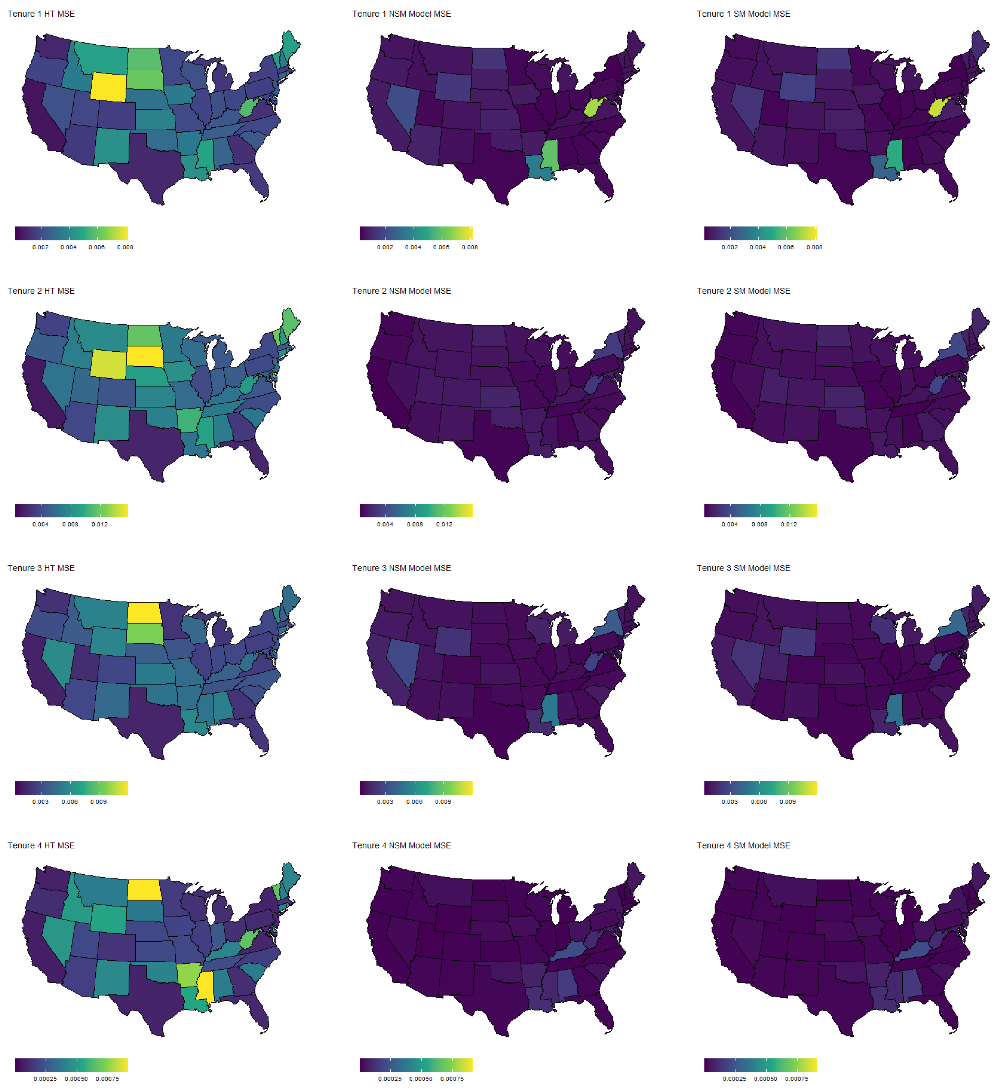
The results of the multinomial simulation are summarized in

Table 2. Collapsed multinomial simulation MSE, squared bias, and 95% credible interval coverage rate. The results are averaged across 49 geographic areas and four categories. Simulated data are based on Week 1 of the Household Pulse Survey.

	MSE	Bias${}^2$	Coverage
NSM Model	0.00074	0.00034	0.932
SM Model	0.00074	0.00033	0.933
HT Estimator	0.00352	0.00004	–

and

Table 3. Multinomial simulation MSE, squared bias, and 95% credible interval coverage rate by category (1–4). The results are averaged across the 49 geographic areas. Simulated data are based on Week 1 of the Household Pulse Survey.

	MSE 1	Bias${}^2$ 1	Cov. 1	MSE 2	Bias${}^2$ 2	Cov. 2	MSE 3	Bias${}^2$ 3	Cov. 3	MSE 4	Bias${}^2$ 4	Cov. 4
NSM Model	0.00083	0.00053	0.945	0.00111	0.00032	0.979	0.00100	0.00050	0.95	0.00003	2.5 × 10−5	0.854
SM Model	0.00079	0.00047	0.950	0.00115	0.00036	0.972	0.00098	0.00046	0.95	0.00003	2.5 × 10−5	0.860
HT Estimator	0.00282	0.00004	–	0.00682	0.00007	–	0.00412	0.00003	–	0.00031	3.0 × 10−6	–

. Table 2 shows the results averaged across samples, states, and categories, whereas Table 3 shows separate summaries for each category. In general, we see that both model-based estimators yield vastly superior estimates in terms of MSE, regardless of the response category. The coverage rates are slightly below the nominal level, although not unreasonable. Response category four has the lowest coverage rate, corresponding to people that rent but cannot pay. This is generally the smallest category, and thus sample sizes are likely an issue here. Finally, for each estimator, we plotted the MSE by state and response category in Figure 2. Again, we see a substantial reduction in MSE for nearly every state and every category. Similar to the binomial case, the largest reductions occur in the states with smaller populations.

4. Household Pulse Survey Analysis

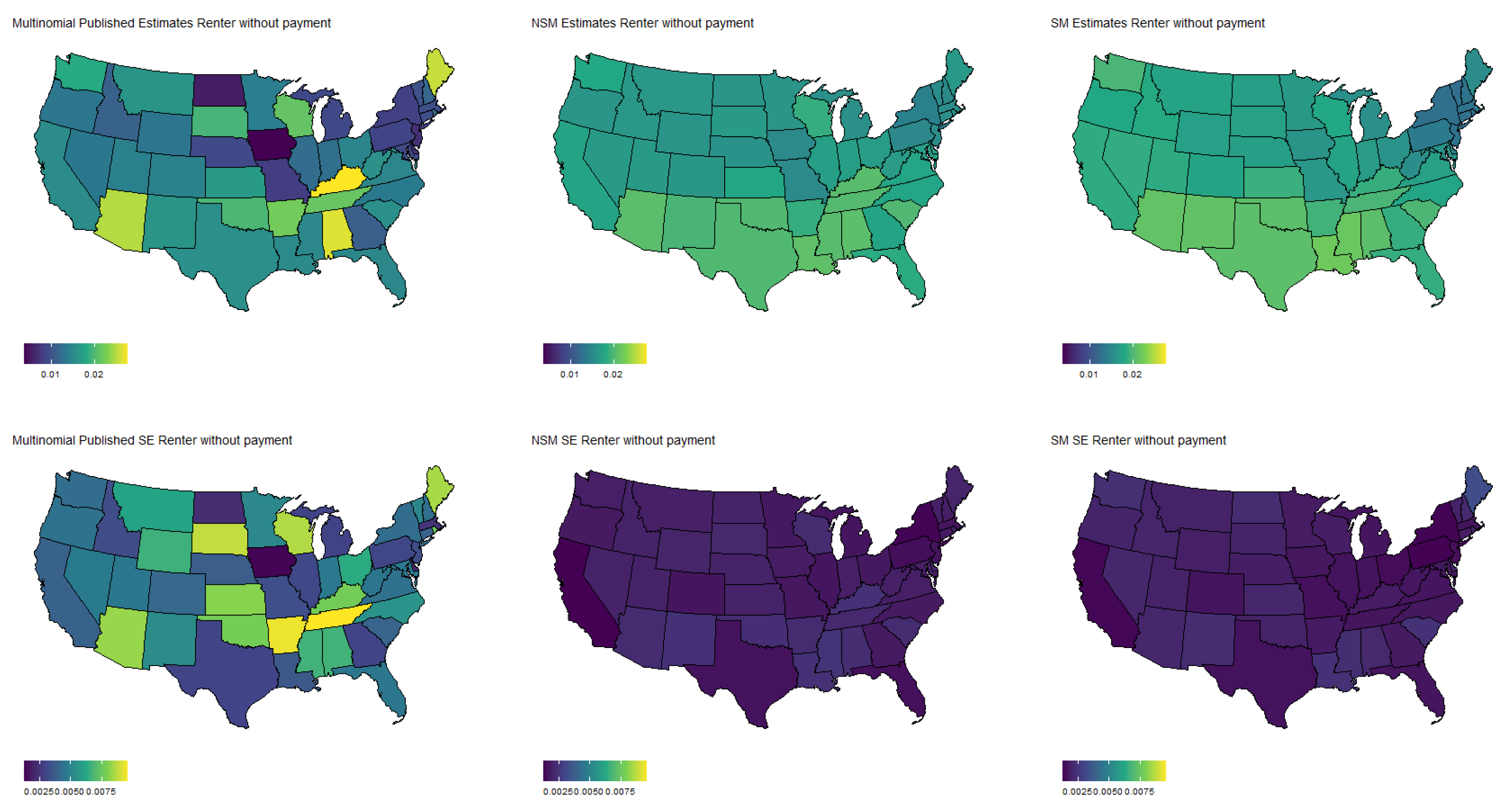
To further illustrate our approach, we analyze the original Household Pulse Survey data. Similar to the simulation, we analyze week one of the public-use HPS data. All priors used and assessment of convergence mirrored those stated in Section 3. The results of this analysis are displayed in Figure 3, Figure 4, Figure 5, Figure 6 and Figure 7.

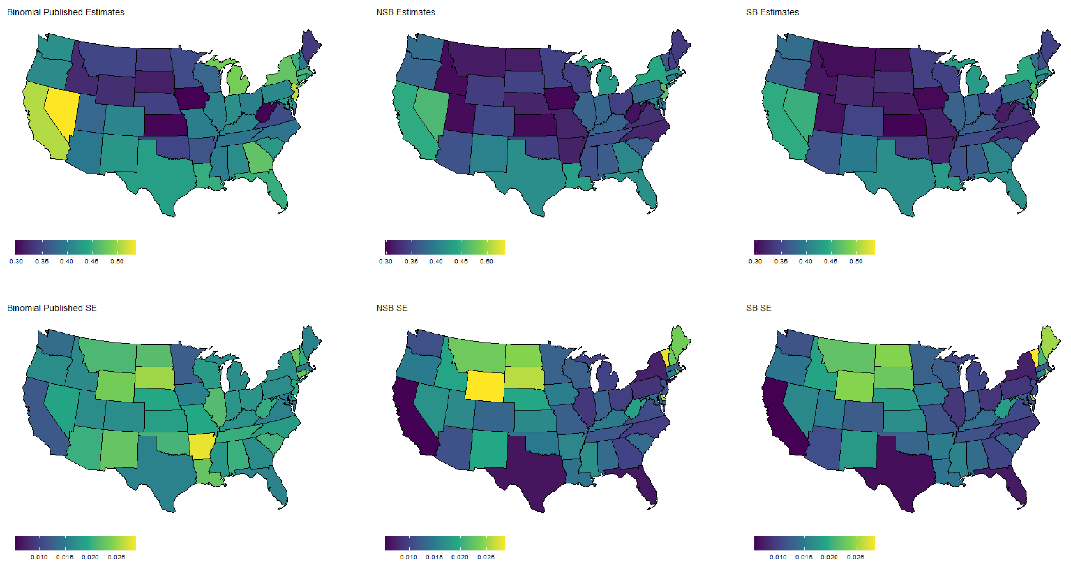
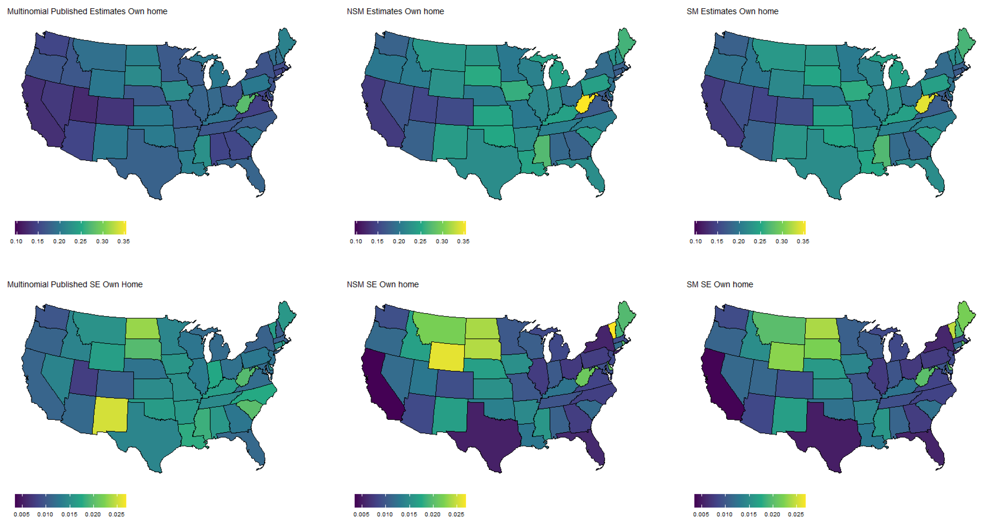
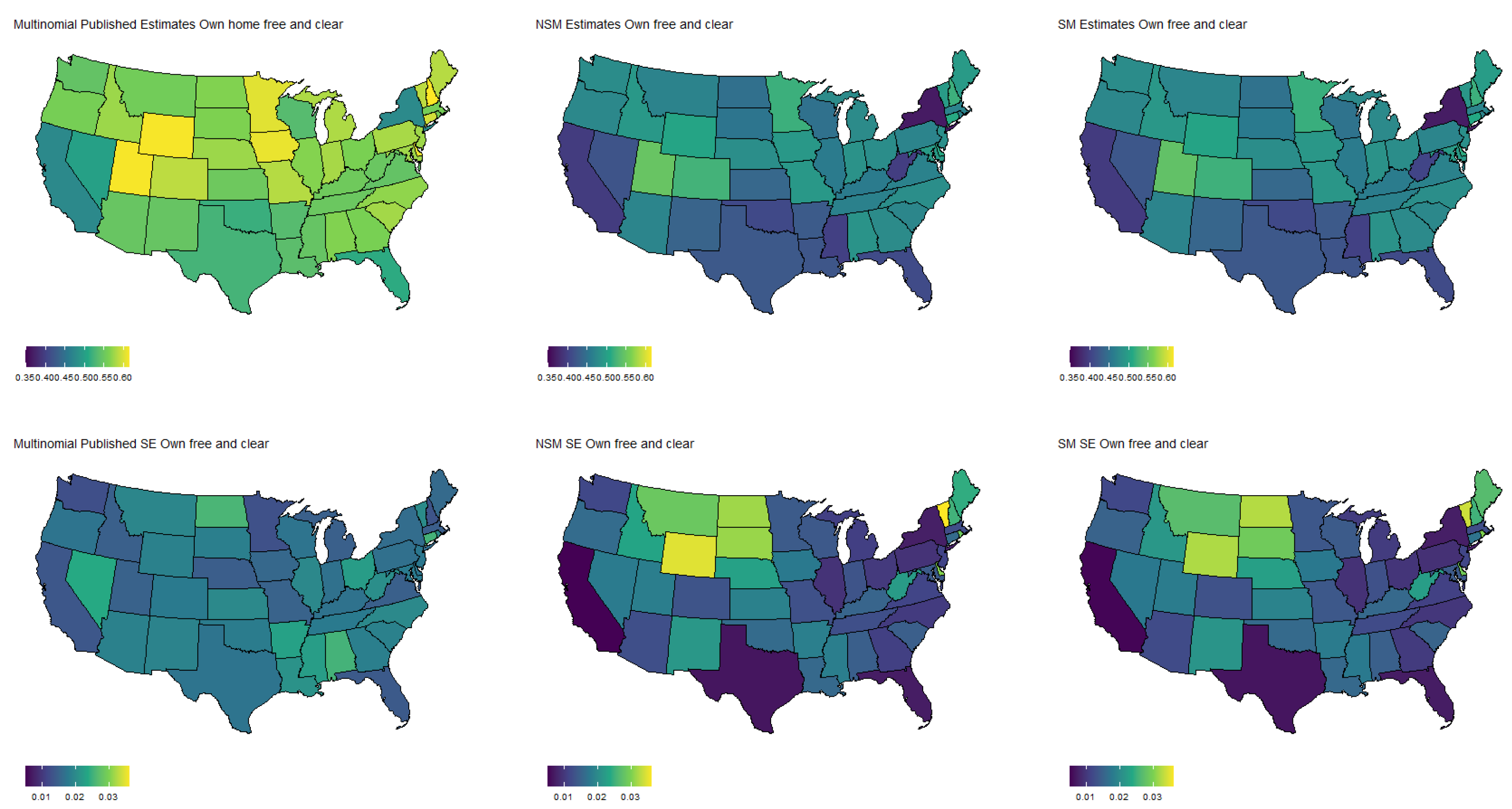
Specifically, Figure 3 shows the population proportion estimates, as well as standard errors, for the binary response “expected job loss”. Meanwhile, Figure 4, Figure 5, Figure 6 and Figure 7 show the estimated population proportions and standard errors for the categorical response “financial living arrangement” with four categories: mortgage, own, rent, rent but cannot pay. As seen in Figure 3, Figure 4, Figure 5, Figure 6 and Figure 7, the spatial pattern produced by the model-based estimator is generally consistent with the direct-estimates for all the cases considered, however the model-based estimates exhibit much less variability, especially in states with a low population. Furthermore, the model-based approach can achieve lower standard errors for both binomial and multinomial responses when compared to the published standard errors of the HPS direct-estimates. Although both model-based estimates are quite similar, in some cases, it does appear that the spatial model is able to leverage dependence structure to achieve slightly reduced standard errors. These results seem to be consistent with our empirical simulations, in which the model-based estimates exhibited a lower MSE.

These results indicate that states that heavily rely on tourism, such as Nevada, California, and Florida, are disproportionately affected by potential job loss due to COVID. Simultaneously, southern states such as Louisiana, Mississippi, and Alabama appear to have the highest rates of people that rent but cannot pay. Estimates such as these could aid in the dispersion of critical resources related to job loss and renter help.

5. Discussion

In this work, we show that model-based estimation often produces superior estimates, in terms of precision, compared to design-based techniques for the HPS. That is, we are able to see reductions in MSE and standard errors for both binomial and multinomial responses. Furthermore, we illustrate that this class of unit-level models for non-Gaussian survey data may be easily fit using Hamiltonian Monte Carlo via Stan, rather than relying on custom sampling software.

Contemporary barriers of sampling, where response rates are low and vary among subgroups, require statisticians to innovate novel model-based approaches that leverage various sources of dependence. For example, we compare non-spatial models with spatially correlated random effects. In this case, there were only very slight advantages to the spatial model structure; however, we would expect much more pronounced gains in efficiency for estimates at a finer spatial resolution (i.e., county or Census tracts, rather than state).

Further model refinements are possible and will be the subject of future research. For example, in Phase 1, it would be possible to leverage temporal dependence in the follow-up interview to further improve the precision of the tabulated estimates. Additionally, model-based estimates that improve the weights constitute another area of potential research. Given the importance of the HPS, and other similar surveys (e.g., RANDS), we expect further opportunities for methodological advancements in unit-level models for survey data from informative samples.

References

1. Centers for Disease Control and Prevention. COVIDView: A Weekly Surveillance Summary of U.S. COVID-19 Activity. 2020. Available online: https://www.cdc.gov/coronavirus/2019-ncov/covid-data/covidview/index.html (accessed on 4 January 2022).
2. U.S. Census Bureau. Household Pulse Survey Microdata. 2020. Available online: https://www.census.gov/programs-surveys/household-pulse-survey/datasets.html (accessed on 4 January 2022).
3. National Center for Health Statistics. Health Care Access, Telemedicine, and Loss of Work Due to Illness. 2020. Available online: https://www.cdc.gov/nchs/covid19/rands.htm (accessed on 4 January 2022).
4. 116th Congress. H.R.133 Consolidated Appropriations Act. 2021. Available online: https://www.congress.gov/bill/116th-congress/house-bill/133/text (accessed on 4 January 2022).
5. 117th Congress. H.R.1319 American Rescue Plan Act. 2021. Available online: https://www.congress.gov/bill/117th-congress/house-bill/1319/text (accessed on 4 January 2022).
6. Rao, J.N.; Molina, I. Small Area Estimation; John Wiley & Sons: Hoboken, NJ, USA, 2015. [Google Scholar]
7. FayIII, R.E.; Herriot, R.A. Estimates of income for small places: An application of James-Stein procedures to census data. J. Am. Stat. Assoc. 1979, 74, 269–277. [Google Scholar] [CrossRef]
8. Battese, G.E.; Harter, R.M.; Fuller, W.A. An error-components model for prediction of county crop areas using survey and satellite data. J. Am. Stat. Assoc. 1988, 83, 28–36. [Google Scholar] [CrossRef]
9. Molina, M. Sae: An R Package for Small Area Estimation. R J. 2015, 7, 81. [Google Scholar] [CrossRef] [Green Version]
10. Namazi-Rad, M.-R.; Steel, D. What level of statistical model should we use in small area estimation? Aust. N. Zeal. J. Stat. 2015, 57, 275–298. [Google Scholar] [CrossRef]
11. Pfeffermann, D.; Sverchkov, M. Small-area estimation under informative probability sampling of areas and within the selected areas. J. Am. Stat. Assoc. 2007, 102, 1427–1439. [Google Scholar] [CrossRef] [Green Version]
12. Parker, P.A.; Janicki, R.; Holan, S.H. Unit level modeling of survey data for small area estimation under informative sampling: A comprehensive overview with extensions. arXiv Prepr. 2019, arXiv:1908.10488. [Google Scholar]
13. Binder, D.A. On the variances of asymptotically normal estimators from complex surveys. Int. Stat. Rev. 1983, 51, 279–292. [Google Scholar] [CrossRef]
14. Skinner, C.J. Domain means, regression and multivariate analysis. In Analysis of Complex Surveys; Skinner, C.J., Holt, D., Smith, T.M.F., Eds.; Wiley: Chichester, UK, 1989; pp. 80–84. [Google Scholar]
15. Zhang, X.; Holt, J.B.; Lu, H.; Wheaton, A.G.; Ford, E.S.; Greenlund, K.J.; Croft, J.B. Multilevel regression and poststratification for small-area estimation of population health outcomes: A case study of chronic obstructive pulmonary disease prevalence using the behavioral risk factor surveillance system. Am. J. Epidemiol. 2014, 179, 1025–1033. [Google Scholar] [CrossRef] [PubMed] [Green Version]
16. Si, Y.; Pillai, N.S.; Gelman, A. Bayesian nonparametric weighted sampling inference. Bayesian Anal. 2015, 10, 605–625. [Google Scholar] [CrossRef] [Green Version]
17. Vandendijck, Y.; Faes, C.; Kirby, R.; Lawson, A.; Hens, N. Model-based inference for small area estimation with sampling weights. Spat. Stat. 2016, 18, 455–473. [Google Scholar] [CrossRef] [Green Version]
18. Parker, P.A.; Holan, S.H.; Janicki, R. Conjugate Bayesian unit-level modelling of count data under informative sampling designs. Stat 2020, 9, e267. [Google Scholar] [CrossRef] [Green Version]
19. Computationally Efficient Bayesian Unit-Level Models for Non-Gaussian Data Under Informative Sampling with Application to Estimation of Health Insurance Coverage. To Appear.—Ann. Appl. Stat. 2022.
20. Porter, A.T.; Wikle, C.K.; Holan, S.H. Small area estimation via multivariate Fay–Herriot models with latent spatial dependence. Aust. N. Zeal. J. Stat. 2015, 57, 15–29. [Google Scholar] [CrossRef] [Green Version]
21. Bradley, J.R.; Holan, S.H.; Wikle, C.K. Multivariate spatio-temporal models for high-dimensional areal data with application to longitudinal employer-household dynamics. Ann. Appl. Stat. 2015, 9, 1761–1791. [Google Scholar] [CrossRef]
22. Carpenter, B.; Gelman, A.; Hoffman, M.D.; Lee, D.; Goodrich, B.; Betancourt, M.; Brubaker, M.; Guo, J.; Li, P.; Riddell, A. Stan: A probabilistic programming language. J. Stat. Softw. 2017, 76, 1–32. [Google Scholar] [CrossRef] [Green Version]
23. Source and Accuracy Statement. 2020. Available online: https://www2.census.gov/programs-surveys/demo/technical-documentation/hhp/Source-and-Accuracy-Statement-April-23-May-5-and-May-7-May12.pdf (accessed on 4 January 2022).
24. Lohr, S.L. Sampling: Design and Analysis: Design And Analysis; CRC Press: Boca Raton, FL, USA, 2019. [Google Scholar]
25. Horvitz, D.G.; Thompson, D.J. A generalization of sampling without replacement from a finite universe. J. Am. Stat. Assoc. 1952, 47, 663–685. [Google Scholar] [CrossRef]
26. Judkins, D.R. Fay’s method for variance estimation. J. Off. Stat. 1990, 6, 223–239. [Google Scholar]
27. Savitsky, T.D.; Toth, D. Bayesian estimation under informative sampling. Electron. J. Stat. 2016, 10, 1677–1708. [Google Scholar] [CrossRef]
28. Besag, J. Spatial interaction and the statistical analysis of lattice systems. J. R. Stat. Soc. Ser. (Methodol.) 1974, 36, 192–225. [Google Scholar] [CrossRef]
29. Midzuno, H. On the sampling system with probability proportionate to sum of sizes. Ann. Inst. Stat. Math. 1951, 3, 99–107. [Google Scholar] [CrossRef]
30. Tillé, Y.; Matei, A. Survey Sampling; R Package Version; R Package: Boston, MA, USA, 2012; Volume 2. [Google Scholar]
31. Stan Development Team. RStan: The R Interface to Stan, R package version 2.21.2; R Package: Boston, MA, USA, 2020. [Google Scholar]
32. Vehtari, A.; Gelman, A.; Simpson, D.; Carpenter, B.; Bürkner, P.-C. Rank-Normalization, Folding, and Localization: An Improved Rˆ for Assessing Convergence of MCMC (with Discussion). Bayesian Anal. 2021, 16, 2. [Google Scholar] [CrossRef]
33. Little, R.J. Post-stratification: A modeler’s perspective. J. Am. Stat. Assoc. 1993, 88, 1001–1012. [Google Scholar] [CrossRef]
Figure 1. Map of MSE by state for each estimator. Data are based on the binomial simulation using Week 1 of the Household Pulse Survey. The response variable used is the expected loss of job and/or income in the next week.
Stats 05 00010 g001
Figure 2. Map of MSE by state for each estimator and category. Data are based on the multinomial simulation using Week 1 of the Household Pulse Survey. The response variable is the housing status: own home with mortgage, own home free and clear, rent, and rent but unable to pay.
Stats 05 00010 g002
Figure 3. Estimated population proportion of people who expect to lose their job by state and estimator along with corresponding standard error for Week 1 of the Household Pulse Survey. Estimates are plotted on the same color scale, and standard errors (SEs) are plotted on another color scale.
Stats 05 00010 g003
Figure 4. Estimated population proportion of people who have a home mortgage by state (excluding Alaska and Hawaii) and D.C. for each estimator along with corresponding standard error in Week 1 of the Household Pulse Survey. Estimates are plotted on the same color scale, and SEs are plotted on another color scale.
Stats 05 00010 g004
Figure 5. Estimated population proportion of people who own their home free and clear by state and estimator along with corresponding standard error in Week 1 of the Household Pulse Survey. Estimates are plotted on the same color scale, and SEs are plotted on another color scale.
Stats 05 00010 g005
Figure 6. Estimated population proportion of people who pay rent by state and estimator along with corresponding standard error in Week 1 of the Household Pulse Survey. Estimates are plotted on the same color scale, and SEs are plotted on another color scale.
Stats 05 00010 g006
Figure 7. Estimated population proportion of people who rent but cannot pay by state and estimator along with corresponding standard error in Week 1 of the Household Pulse Survey. Estimates are plotted on the same color scale, and SEs are plotted on another color scale.
Stats 05 00010 g007