Article

Optimal Investment and Consumption for Multidimensional Spread Financial Markets with Logarithmic Utility

by
Sahar Albosaily
1 and
Serguei Pergamenchtchikov
2,3,*
1
Department of Mathematics, Faculty of Science, University of Ha’il, Ha’il P.O. Box 2440, Saudi Arabia
2
Laboratoire de Mathématiques Raphael Salem, UMR 6085 CNRS-Université de Rouen, F76801 Saint-Étienne-du-Rouvray, France
3
International Laboratory of Statistics of Stochastic Processes and Quantitative Finance, Tomsk State University, 634050 Tomsk, Russia
*
Author to whom correspondence should be addressed.
Stats 2021, 4(4), 1012-1026; https://doi.org/10.3390/stats4040058
Submission received: 22 October 2021 / Revised: 21 November 2021 / Accepted: 26 November 2021 / Published: 29 November 2021
(This article belongs to the Special Issue Statistical Analysis of Econometrics)

Abstract

:
We consider a spread financial market defined by the multidimensional Ornstein–Uhlenbeck (OU) process. We study the optimal consumption/investment problem for logarithmic utility functions using a stochastic dynamical programming method. We show a special verification theorem for this case. We find the solution to the Hamilton–Jacobi–Bellman (HJB) equation in explicit form and as a consequence we construct optimal financial strategies. Moreover, we study the constructed strategies with numerical simulations.

1. Introduction

In this paper, we consider an optimisation and consumption problem for spread financial markets on the time interval [ 0 , T ] . Our goal is to find investment and consumption strategies which maximise the terminal wealth and the consumption during the investment period for logarithmic utilities. The spread means the difference between two prices of co-integrated risky assets (see, for example, in [1,2]). The co-integration property for time series means that the difference between them represents a stationary process. If we consider two or more stocks that are selected for the joint integration and correlation between them, then multidimensional stationary processes should be used. In discrete time, multivariate stationary processes can be well approximated by auto-regressive models in R d
X n = A X n 1 + ξ n ,
where ( ξ n ) n 1 are i.i.d. random zero mean vectors in R d . In continuous time, this model corresponds to the stochastic differential equation in R d (see, for example, [3,4]), i.e.,
d X t = A X t d t + σ d W t ,
where W t is a standard Brownian motion. This equation is called the Ornstein–Uhlenbeck (OU) process in R d . Thus, it is very natural to use such processes to model the spread markets in continuous time with the stable matrix A, i.e., when all the eigenvalues have negative real parts. It should be noted that in this case, the spread is a mean-reverting process, therefore, if investors sell high stocks (with high prices) and buy low stocks (with low prices) when the spread widens, then this will assure the continuity of profits over time in such market models. Thus, the idea is to go long when the price is under the long-term mean and go short for the stock price over the long-term mean, as reciprocal actions for the chosen co-integrated stocks. Moreover, it should be noted that the spread trade is much cheaper than trading stocks directly since for spread strategies, transaction costs are paid for two stocks at once, while for the direct trading in stocks, transaction costs are paid for each stock separately. The notion of spread markets goes back to the 1980’s where the team of Nunzio Tartaglia at Morgan Stanley proposed the pairs trading idea to take advantage of market mispricing to gain profit [5,6]. Several studies have been using the notion of spread to examine the behaviour of financial markets. Indeed, the spread markets are very popular in the financial industry, for example, for the precious metals spread [7], the oil markets spread [8,9], in other sectors like the microstructure level [10] and in many hedge funds [2]. The choice of pairs is quite important; they have to be correlated and have a certain pattern history so that the spread between them is mean reverting. The choice of pairs is not the goal of this paper. We only emphasise that some articles discussed the tests that have been used in order to choose pairs (see for example [11]). Our goal is to study portfolio optimisation problems for spread markets. According to the classical mathematical economics problem (see for example [12]), in this paper we consider the optimal investment and consumption problem. Note that for the Black–Scholes (BS) and stochastic volatility markets, such problems are considered in many papers (see for example [12,13,14,15]). In addition, affine processes have been proposed in [14,16] to be used in the financial markets in a general framework; however, unfortunately we can not use these methods due to the additional variables in the Hamilton–Jacobi–Bellman (HJB) equation corresponding to the spread asset. The idea of pairs trading is widely used; however, the academic research about it is still scarce [17]. In this paper, we are concerned about the stochastic control approach for spread markets. We consider the case of logarithm utility functions for the optimal investment–consumption problem with no constraints or transaction fees over the whole investment interval. Note that for power utilities, such problems are studied in different settings in [1,18]. The main difference between the spread markets and BS and stochastic volatility models is that the HJB equation has an additional multivariate spread variable. Therefore, we need to develop new analytical methods for such optimisation problems. First, according to the stochastic dynamical programming method, we study the HJB equation and we obtain its solution in an explicit form. Then, we show a special new verification theorem for this case, and finally, by making use of this theorem, we construct optimal strategies.
The rest of the paper is organised as follows. In Section 2 we formulate the problem and we define the spread process under the Ornstein–Uhlenceck model. In Section 3, we write the HJB equation and we demonstrate its solution in an explicit form. The main results of this paper are stated in Section 4 and some numerical simulations are given in Section 5. The corresponding verification theorem is stated in Section 6.

2. Market Model

Let ( Ω , F T , ( F t ) 0 t T , P ) be a standard filtered probability space with ( F t ) 0 t T adapted Wiener processes W = ( W t ) 0 t T R m . Our financial market consists of one riskless bond  ( B t ) 0 t T and risky spread asset  ( S t ) 0 t T governed in R d by the following differential equations:
d B t = r B t d t , B 0 = 1 , d S t = A S t d t + σ d W t , S 0 > 0 ,
where r 0 is the interest rate for riskless asset, S t = ( S 1 ( t ) , S 2 ( t ) , S 3 ( t ) , , S d ( t ) ) are the risky assets, ( W t ) 0 t T is the standard Brownian motion with values in R m , the volatility σ is a d × m matrix such that ( σ σ ) 1 exists, denotes the transposition and the d × d mean-reverting matrix A
A = a 11 a 12 a 1 d a 21 a 22 a 2 d a d 1 a d 2 a d d .
We assume that
sup x R d x A x | x | 2 < 0 .
Note that this condition implies that the real parts of the eigenvalues are negative, i.e., R e λ i ( A ) < 0 . Let now β t be the value of the riskless asset B t at the time moment 0 t T and α t = ( α 1 ( t ) , α 2 ( t ) , , α d ( t ) ) R d be the number of risky assets at the moment 0 t T , and the consumption rate is given by a non-negative integrated function ( c t ) 0 t T [12]. Thus, the wealth process for X t = β t B t + α t S t is given by
d X t = β t d B t + α t d S t c t d t ,
which can be written as
d X t = ( r X t α t S ^ t c t ) d t + α t σ d W t ,
where S ^ t = A 1 S = ( S ^ 1 ( t ) , , S ^ d ( t ) ) R d and A 1 = r I d A . Note that in this case the matrix A 1 is invertible, i.e., there exists A 1 1 . In the following, we denote the financial strategy by υ t = ( α t , c t ) Θ = R d × R + and the wealth process (3) corresponding to this strategy by X t υ . Moreover, we set ς t υ = ( X t υ , S t ) R n , where n = d + 1 . In this paper, we use the logarithmic utility functions, i.e., we need the following definition for the admissible strategies.
Definition 1.
The strategy υ = ( υ t ) 0 t T is called admissible if it is adapted and such that
j = 1 d 0 T α j 2 ( t ) d t + 0 T c t d t < a . s .
and Equation (3) has a unique non-negative strong solution and the following conditions hold
E 0 T ( ln c t ) d t < + a n d E sup 0 t T ( ln ( X t υ ) ) < + ,
where ( x ) is the negative part of x, i.e., ( x ) = min ( 0 , x ) . We denote by V the set of all admissible strategies.
Now, for any υ V and ς = ( x , s ) from Ξ = R + × R d , we define the objective function as
J ( ς , υ ) : = E ς 0 T ( ln c u ) d u + ϖ ln ( X T υ ) ,
where E ς is the expectation under condition ς 0 υ = ς . Our goal in this paper is to maximise this function, i.e.,
J * ( ς ) : = sup υ V J ( ς , υ ) .
To study this problem we use the stochastic dynamic programming method. To this end we need to consider the optimisation problems on the interval [ t , T ] for any 0 t < T . For the problem on the interval [ t , T ] we use the strategies υ from V such that the process ( υ u ) t u T is adapted to the field family ( F t , u ) t u T , where F t , u = σ { W v W t , t v u } . The class of such strategies is denoted by V t . Then, we need to study the value functions ( J * ( ς , t ) ) 0 t T defined as
J * ( ς , t ) = sup υ V t E ς , t t T ( ln c u ) d u + ϖ ln ( X T υ ) ,
where ϖ > 0 and E ς , t is the expectation under condition ς t υ = ς = ( x , s ) Ξ . Thus, we need to study the HJB equation which is given in the following section.

3. Hamilton–Jacobi–Bellman Equation

Using the process ς t υ , we can rewrite the wealth and stock equations given in (1) and (3), respectively, in the following form
d ς t υ = a ( ς t υ , υ t ) d t + b ( ς t υ , υ t ) d W t , ς 0 = ς ,
where a R n and b is the matrix of n × m functions such that for any ς = ( x , s ) Ξ
a ( ς , u ) = r x α s ^ c s ˜ a n d b ( ς , u ) = α σ σ ,
where s ^ = A 1 s , and we denote by s ˜ = A s = ( s ˜ 1 , , s ˜ d ) R d , the control variable u = ( α , c ) with α R d and c > 0 . For any q = ( q 1 , , q n ) R n and n × n symmetric matrix M = ( M i j ) 1 i , j N , we set the Hamilton function as
H ( ς , q , M ) : = sup u Θ H 0 ( ς , q , M , u ) , Θ = R d × R + ,
where
H 0 ( ς , q , M , u ) : = a ( ς , u ) q + 1 2 tr [ b b ( ς , u ) M ] + ln c .
In order to study problem (5), we need to solve the HJB equation which is given by:
z t ( ς , t ) + H ( ς , z ( ς , t ) , 2 z ( ς , t ) ) = 0 , t [ 0 , T ] , z ( ς , T ) = ϖ ln x , ς R n ,
where z ( ς , t ) = ( z x , z s 1 , , z s d ) R n and
2 z ( ς , t ) = z x x z x s 1 z x s 2 z x s d z x s 1 z s 1 s 1 z s 1 s 2 z s 1 s d z x s d z s d s 1 z s d s 2 z s d s d n × n .
To calculate the Hamilton function (7), note that
H 0 ( ς , q , M , υ ) = ( r x α s ^ c ) q 1 + i = 1 d s ˜ i q 1 + i + 1 2 ( α σ σ α M 11 + 2 i = 1 d < σ σ α > i M 1 , 1 + i + k , i = 1 d < σ σ > k i M 1 + k , 1 + i ) + ln c .
The symbol < X > i denotes the i-th element of the vector X and < Y > i j denotes the ( i , j ) element of the matrix Y. Note that due to (7), if M 11 0 or q 1 0 , then the Hamilton function H ( ς , q , M ) = + . Therefore, we maximise the function H 0 ( ς , q , M , υ ) over α and c under the conditions that M 11 < 0 and q 1 > 0 . We obtain that optimal values for this maximisation problem are given by
α 0 ( s , q , M ) = ( σ σ ) 1 τ M 11 a n d c 0 ( s , q , M ) = 1 q 1 ,
where τ = q 1 s ^ σ σ μ and μ = ( M 1 , 2 , , M 1 , 1 + d ) . Now we replace α i 0 and c 0 into H 0 to obtain the Hamilton function:
H ( ς , q , M ) = r x q 1 ln q 1 + τ ( σ σ ) 1 τ 2 | M 11 | + i = 1 d s ˜ i q 1 + i + 1 2 k , i = 1 d < σ σ > k i M 1 + i , 1 + k 1 .
From the preceding Hamilton function and the HJB Equation (8) and setting
τ ^ = z x s ^ σ σ μ ^ a n d μ ^ = ( z x , s 1 , , z x , s d ) ,
we obtain
z t + r x z x + τ ^ ( σ σ ) 1 τ ^ 2 | z x x | 1 ln z x + i = 1 d s ˜ i z s i + 1 2 k , i = 1 d < σ σ > k i z s i s k = 0 ,
where z ( ς , T ) = ln x for any ς Ξ . To write the solution for this equation, we need to introduce the d × d matrix g = ( g i j ) 1 i , j d which is the solution of the following differentiable equation
g ˙ + 1 2 ρ A 1 ( σ σ ) 1 A 1 + g 1 A = 0 , g ( T ) = 0 ,
where g ˙ denotes the derivative of g, ρ = ρ ( t ) = T t + 1 and g 1 = g + g . Moreover, we need the following differential equation:
f ˙ + r ρ + t r σ σ g 1 ln ρ = 0 , f ( T ) = 0 ,
where t r denotes the trace of the matrix. We show that Equation (9) has the following solution:
z ( x , s , t ) = ρ ( t ) ln x + s g ( t ) s + f ( t ) .
Here, g is the solution of Equation (10), which can be represented as
g ( t ) = ( T t ) ( T t + 2 ) 4 A 1 ( σ σ ) 1 A 1 + 0 T t G ( v ) d v A
and G ( v ) = 0 v e A u A 1 ( σ σ ) 1 A 1 e A u ( v + 1 u ) d u . The function f in (12) is the solution of (11), which is
f ( t ) = t r σ σ g ˜ ( t ) + r ( T t ) ( T t + 2 ) 2 ρ ( t ) ln ρ ( t ) ,
where g ˜ ( t ) = t T g ( v ) d v .
Remark 1.
As we see in the HJB equation, the additional variable s R d corresponds to the spread assets. This is the main difference from the BS market.

4. Main Results

First, we have to study the HJB Equation (9) to calculate the value function (5).
Theorem 1.
The function (12) satisfies the HJB Equation (8).
Furthermore, to construct the optimal strategies we set
α ˜ ( ς , t ) = α 0 ( ς , z , 2 z ) = ( σ σ ) 1 s ^ x a n d c ˜ ( ς , t ) = c 0 ( ς , z , 2 z ) = x ρ ( t ) .
Recall that s ^ = A 1 s = ( s ^ 1 , , s ^ d ) R d . Using these functions, we define the optimal strategies υ * = ( α * , c * ) as
α * ( t ) = α ˜ ( ς t * , t ) = ( σ σ ) 1 S ^ t X t * a n d c * ( t ) = c ˜ ( ς t * , t ) = X t * ρ ( t ) .
Here ς t * = ( X t * , S t ) and X t * is the optimal wealth process defined by the following stochastic differential equation:
d X t * = X t * a * ( t ) d t + X t * ( b * ( t ) ) d W t , X 0 * = x ,
where
a * ( t ) = r + S ^ t ( σ σ ) 1 S ^ t 1 ρ ( t ) a n d b * ( t ) = σ ( σ σ ) 1 S ^ t .
Now we show that these processes are optimal solutions for problem (5).
Theorem 2.
The processes (14) and (15) are the optimal strategies for problem (5) and
J * ( x , s , t ) = z ( x , s , t ) = ρ ( t ) ln x + s g ( t ) s + f ( t ) ,
where ρ , g and f are given in (10).
Example 1.
For the one-dimensional case, the riskless and risky assets are given, respectively, by
d B t = r B t d t , B 0 = 1 , d S t = κ S t d t + σ d W t , S 0 > 0 ,
where r 0 is the interest rate of the riskless asset, κ > 0 and σ are, respectively, the mean-reverting speed and the volatility for the risky assets. Therefore, for κ 1 = κ + r > 0 , the optimal strategies and the HJB equation are given by
α * ( t ) = α ˜ 0 ( ς t * , t ) = κ 1 S t X t * σ 2 a n d c * ( t ) = c ˜ 0 ( ς t * , t ) = X t * ρ ( t ) .
Moreover, the differential wealth process for this example is given by
d X t * = X t * a * ( t ) d t + X t * b * ( t ) d W t ,
where
a * ( t ) = a ( S t , t ) = r + κ 1 2 S t 2 / σ 2 1 / ρ ( t ) a n d b * ( t ) = b ( S t , t ) = κ 1 S t / σ .
Example 2.
For the multidimensional case where the market assets are given by
d B t = r B t d t , B 0 = 1 , d S t = A S t d t + σ d W t , S 0 > 0 ,
where r is the interest rate for riskless asset B and S t = ( S 1 ( t ) , S 2 ( t ) , S 3 ( t ) , , S d ( t ) ) R d is a d-dimensional vector of risky assets, ( W t ) is a standard Brownian motion with values in R d , the market volatility matrix σ = d i a g ( σ 1 , σ 2 , , σ d ) , and the mean-reverting matrix A is given by
A = a 11 a 12 a 1 d a 21 a 22 a 2 d a d 1 a d 2 a d d
with negative real eigenvalues, i.e., R e λ i ( A ) < 0 . The optimal wealth process ( X t * ) 0 t T is defined by the following stochastic equation
d X t * = X t * a * ( t ) d t + X t * ( b * ( t ) ) d W t , X 0 * = x ,
where
a * ( t ) = r + i = 1 d S ^ i 2 ( t ) σ i 2 1 ρ ( t ) , b * ( t ) = ( b 1 * ( t ) , , b d * ( t ) ) a n d b i * ( t ) = S ^ i ( t ) / σ i .
Using the preceding stochastic differential equation, the optimal strategies υ * = ( α * , c * ) for all 0 t T are of the form:
α i * ( t ) = β i 0 ( ς t * , t ) = S ^ i ( t ) X t * σ i 2 a n d c * ( t ) = c ˜ 0 ( ς t * , t ) = X t * ρ ( t ) ,
where β t is the number of riskless assets B and α t = ( α 1 ( t ) , α 2 ( t ) , , α d ( t ) ) R d are the number of risky assets S at the moment 0 t T .
Remark 2.
It should be noted that the behaviour of these optimal strategies are described by the transformed spread process S ^ t = A 1 S t . In the scalar case this is the same as S t . However, in the general multidimensional case we need to take into account all components of the spread processes.

5. Numerical Simulation

In this section we present numerical simulations for the one-dimensional market (16). For this case, Figure 1 shows the value function z ( ς , t ) given by (12). The following parameters have been used: T = 1 , r = 0.01 , κ = 0.1 , σ = 0.5 and the initial endowment is x = 100 .
Now, we simulate the optimal strategies α t * and c t * given in (14) with the optimal wealth process x t * . In the following figures, we used different parameters to show the behaviour of the strategies with different values of r, κ and σ . The figures below show that the behaviour of the wealth process is increasing constantly when κ has large values. However, it is clear that the wealth process is decreasing when κ has quite a small value. In addition we see that the volatility in the investment process increases and decreases depending on the fraction κ 1 / σ 2 . Thus, the range of volatility in Figure 2b, Figure 3b and Figure 4b is less than in Figure 5b, where it jumps to 4000 points. This is due to the higher number we get from the fraction, which is nearly 50.

6. Verification Theorem

Here we give some modifications to the verification theorem from [15]. Consider on the interval [ 0 , T ] the stochastic control process with its values in Ξ R n
d ς t υ = a ( ς t υ , t , υ t ) d t + b ( t , ς t υ , υ t ) d W t , t 0 , ς 0 υ = x Ξ ,
where ( W t ) 0 t T is a standard m-dimensional Brownian motion and F t = σ { W u , 0 u t } for any 0 < t T . We assume that the control process υ t takes values in some set Θ R q for some integer q 1 . Moreover, we assume that the coefficients a and b satisfy the following conditions:
( V 1 )
For all t [ 0 , T ] , the functions a ( . , t , . ) and b ( . , t , . ) are continuous on R n × Θ .
( V 2 )
For every deterministic vector u Θ , the stochastic differential Equation (17) has a unique strong non-negative solution with υ t u .
Next, we introduce an admissible control process for Equation (17).
Definition 2.
The stochastic control process υ = ( υ t ) 0 t T is called admissible on [ 0 , T ] with respect to (17) if it is ( F t ) 0 t T progressively measurable with values in Θ, and (17) has a unique strong solution, such that ς t Ξ for any 0 t T ,
E 0 T f ( ς u , u , υ u ) d t < + , E sup 0 t T ( h ( ς t υ ) ) < + ,
and
0 T ( | a ( ς u υ , u , υ u ) | + | b ( ς u υ , u , υ u ) | 2 ) d t + 0 T | f ( ς u , u , υ u ) | d u < + a . s .
We denote by V the set of all admissible control processes with respect to Equation (17).
Moreover, let f : Ξ × [ 0 , T ] × Θ R and h : Ξ R be continuous utility functions. We define the cost function by
J ( x , t , υ ) = E x , t t T f ( ς , u , υ u ) d u + h ς T υ , 0 t T ,
where E x , t is the expectation operator conditional on ς t υ = x . Our goal is to solve the optimisation problem (5) given by
J * ( x , t ) : = sup υ V t J ( x , t , υ ) ,
where V t is the class of such strategies υ V such that the process ( υ u ) t u T is adapted to the field family ( F t , u ) t u T , where F t , u = σ { W v W t , t v u } . To this end we introduce a Hamilton function, i.e., for any x and 0 t T , with q R n and symmetric n × n matrix M we set
H ( x , t , q , M ) : = sup θ Θ H 0 ( x , t , q , M , θ ) ,
where
H 0 ( x , t , q , M , θ ) : = a ( x , t , θ ) q + 1 2 t r [ b b ( x , t , θ ) M ] + f ( x , t , θ ) .
In order to find the solution to (5), we investigate the HJB equation
z t ( x , t ) + H ( x , t , z x ( x , t ) , z x x ( x , t ) ) = 0 , t [ 0 , T ] , z ( x , T ) = h ( x ) , x Ξ .
Here, z t denotes the partial derivative of z with respect to t, z x ( x , t ) the gradient vector with respect to x in R n and z x x ( x , t ) denotes the symmetric hessian matrix, that is the matrix of the second order partial derivatives with respect to x. We assume the following conditions hold:
( H 1 )
There exists a Ξ × [ 0 , T ] R function z ( x , t ) from C 2 , 1 Ξ × [ 0 , T ] which satisfies the HJB equation such that for any υ V , any 0 t T and x Ξ ,
E x , t sup t u T ( z ( ς u υ , u ) ) < + .
( H 2 )
There exists a measurable function θ * : R n × [ 0 , T ] Θ , such that for all x R n and 0 t T ,
H ( x , t , z x ( x , t ) , z x x ( x , t ) ) = H 0 ( x , t , z x ( x , t ) , z x x ( x , t ) , θ * ( x , t ) ) .
( H 3 )
There exists a unique strong solution to the Itô equation
d ς t * = a ( ς t * , t ) d t + b ( ς * , t ) d W t , ς 0 * = x , t 0 ,
where a ( . , t ) = a ( . , t , θ * ( . , t ) ) and b ( . , t ) = b ( . , t , θ * ( . , t ) ) . Moreover, the optimal control process υ t * = θ * ( υ t * , t ) for 0 t T belongs to V , and
E x , t sup t u T | z ( ς u * , u ) | < .
Theorem 3.
Assume that conditions ( H 1 )–( H 3 ) hold. Then the process υ t * = ( υ t * ) 0 t T defined in condition ( H 3 ) is a solution to this problem.
 Proof. 
For υ V , let ( ς u υ ) t u T be the associated wealth process with ς t υ = x . For any fixed L > 0 define a stopping time
τ L = inf s t : t s | b ( ς u υ , u ) ς z ( ς u υ , u ) | 2 d u L T .
Note that condition (18) implies that τ L T as L a.s. By the continuity of the functions z ( . , . ) and ( ς t υ ) 0 t T we obtain
lim L z ( ς τ L υ , τ L ) = z ( ς T υ , T ) = h ( ς T υ ) a . s .
To simplify, we use the notation a t υ = a ( ς t , υ t , t ) and b t υ = b ( ς t , υ t , t ) . Then by the Itô formula:
d z ( ς t υ , t ) = z t ( ς t υ , t ) d t + i = 1 n ς i z ( ς t υ , t ) d ς i υ ( t ) + 1 2 i , j = 1 n 2 ς i ς j z ( ς t υ , t ) d < ς i υ , ς j υ > t .
By using (17), the preceding equation becomes:
d z ( ς t υ , t ) = z t ( ς t υ , t ) + ( z ( ς t υ , t ) ) a t υ d t + 1 2 t r ( b t υ ( b t υ ) 2 z ( ς t υ , t ) ) d t + ( z ( ς t υ , t ) ) b t υ d W t .
Taking the integration on both sides we get
z ( ς τ L υ , τ L ) z ( ς t υ , t ) = t τ L D u d u + t τ L ( z ( ς u υ , u ) ) b t υ d W u ,
where D u = z u ( ς u υ , u ) + ( z ( ς u υ , u ) ) a u υ + t r b u υ ( b u υ ) 2 z ( ς u υ , u ) / 2 . Taking into account that E x , t z ( ς t , t ) = z ( x , t ) and
E x , t t τ L ( z ( ς u υ , u ) ) b t υ d W u = 0 ,
we obtain that
z ( x , t ) = E x , t z ( ς τ L υ , τ L ) t τ L D u d u .
Moreover, noting that z u ( x , u ) = H ( x , z x , z x x ) , we can represent the processes D u as:
D u = H ς u υ , z ( ς u υ , u ) , 2 z ( ς u υ , u ) H 0 ς u υ , z ( ς u υ , u ) , 2 z ( ς u υ , u ) , υ u + f ( ς u υ , u , υ u ) .
So, for υ V ,
D u f ( ς u υ , u , υ u ) .
Therefore,
z ( x , t ) E x , t z ( ς τ L υ , τ L ) + t τ L f ( ς u υ , u , υ u ) d u .
As to this term, note that
t τ L f ( ς u υ , u , υ u ) d u = t τ L ( f ( ς u υ , u , υ u ) ) + d u t τ L ( f ( ς u υ , u , υ u ) ) d u .
We recall that
E 0 T ( f ( ς u υ , u , υ u ) ) d u < + .
Therefore, we obtain by the monotone convergence theorem that
lim L E 0 τ L f ( ς u υ , u , υ u ) d u = E t T f ( ς u υ , u , υ u ) d u .
Note also, that in view of the condition ( H 2 ),
E x , t sup L 1 ( z ( ς τ L υ , τ L ) ) E x , t sup t u T ( z ( ς u υ , u ) ) < + .
Therefore, by Fatou’s Lemma we obtain that
lim L E x , t z ( ς τ L υ , τ L ) E x , t lim L z ( ς τ L υ , τ L ) = E x , t z ( ς T υ , T ) = E x , t h ( ς T υ ) .
Finally, we obtain that
z ( x , t ) E x , t t T f ( ς u υ , u , υ u ) d u + h ( ς T υ ) = J ( x , t , υ ) .
Therefore, z ( x , t ) J * ( x , t ) for all 0 t T . Similarly, replacing the strategies υ given by the optimal strategies υ * as defined in ( H 2 ) and ( H 3 ) we obtain:
z ( x , t ) = E x , t t τ L f ( ς u * , u , υ u * ) d u + E x , t z ( ς τ L * , τ L ) .
The upper bound (19) implies that the family { z ( ς τ L * , τ L ) } L 1 is uniformly integrable. Therefore, the limit Equation (20) yields
lim L E x , t z ( ς τ L * , τ L ) = E x , t lim L z ( ς τ L * , τ L ) = E z ( ς T υ , T ) = E x , t h ( ς T * ) ,
and we obtain
z ( x , t ) = lim L E x , t t τ L f ( ς u * , u , υ u * ) d u + lim L E x , t z ( ς τ L * , τ L ) = E x , t t T f ( ς u * , u , υ u * ) d u + h ( ς T * ) = J ( x , t , υ * ) .
We arrive at z ( x , t ) = J * ( x , t ) . This proves (3). □
Remark 3.
The difference in (3) from the verification theorem from [15] is that the functions f and h are positive but from the logarithmic utilities these functions are negative. As a result, we can not use the verification theorem in [15] directly.

7. Proofs

Proof of Theorem 1.
By taking the derivatives of z ( ς , t ) defined in (12) with respect to t and s and by applying them into Equation (9) we obtain
s g ˙ ( t ) s + f ˙ ( t ) + r ρ ( t ) + t r σ σ g ln ρ ( t ) 1 + j = 1 d l = 1 d A j l s l < g 1 > i k + ρ ( t ) s ^ ( σ σ ) 1 s ^ 2 = 0 ,
where g is a d × d matrix defined in. Then this can be written as
s ( g ˙ ( t ) + 1 2 ρ ( t ) A 1 ( σ σ ) 1 A 1 g 1 A ) s + f ˙ ( t ) + r ρ ( t ) + t r σ σ g 1 ln ρ ( t ) = 0 .
Therefore, taking into account the differential Equations (10) and (11), we obtain the solution of the HJB Equation (9) in the form (12). Now, we study Equation (10). To this end, we note, that the matrix g is not generally symmetric. For that reason, we first study the equation for the symmetric matrix g 1 = g + g . From (10) it follows that
g ˙ 1 + ρ D + A g 1 + g 1 A = 0 , g 1 ( T ) = 0 ,
where D = A 1 ( σ σ ) 1 A 1 . Using the solutions for the homogeneous matrix linear differential equations (see for example [19]) we can obtain that
g 1 ( t ) = e A t t T e A s D e A s ρ ( s ) d s e A t = G ( T t ) ,
where the matrix G is defined in (13). Using this matrix in (10) we get the form (13). This proves Theorem 1. □
Proof of Theorem 2.
We apply the verification (3) to Problem (5) for the stochastic control differential Equation (6). First note that from the definition of the risk asset in (1), it follows that for t < u < T and s R d
S u = e A ( u t ) s + ξ t , u a n d ξ t , u = t u e A ( u v ) σ d W v .
It should be noted that the upper bound (1.1.11) of Proposition 1.1.2 in [4] implies directly that
E sup t u T | ξ t , u | 2 < .
Therefore, (1) and the last inequality in (4) imply the condition H 1 . Moreover, note that the linear Equation (15) has the strong unique solution X t * given as
X t * = x exp 0 t a * ( u ) b * ( u ) 2 / 2 d u + 0 t ( b * ( u ) ) d W u .
Therefore, the strategy υ * = ( υ t * ) 0 t T with υ t * = ( α t * , c t * ) defined in (14) and (15) belongs to the class V and satisfies the condition H 2 . To check the condition H 3 we have to show the upper bound (19), i.e.,
E ς , t sup t u T | z ( ς u * , u ) | <
for any ς R + × R n . Taking into account that in the HJB solution (12) the functions g and f are bounded, it suffices to check that
E ς , t sup t u T | ln ( X u * ) | + | S u | 2 < .
Therefore, in view of (22) and (23), one needs to check that
E ς , t sup t u T | ln ( X u * ) | < .
For this, taking into account the representation (24), it suffices to check that
E ς , t t T | a * ( u ) | + b * ( u ) 2 d u + E ς , t sup t u T t u ( b * ( v ) ) d W v 2 < .
Note now that from the definition of the functions a * ( t ) and b * ( t ) in (15) and the conditions of this theorem, we have that
| a * ( t ) | c 1 ( 1 + | S t | 2 ) a n d | b * ( t ) | c 2 | S t |
for some constant c 1 > 0 and c 2 > 0 . Moreover, using Doob’s martingale inequality, the equality (23) and the bound (22), we obtain that
E ς , t sup t u T t u ( b * ( v ) ) d W v 2 4 E ς , t t T ( b * ( u ) ) d W u 2 = 4 E ς , t t T | b * ( u ) | 2 d u < .
This proves (2). □

8. Conclusions

In conclusion, we emphasize, that in this paper, the investment and consumption problem for the multivariate spread financial market (1) for the logarithmic utility functions is studied on the basis of stochastic dynamic programming method. To this end, we obtained the HJB Equation (9) and we found the explicit form for its solution in (12). Then, using this solution and the verification theorem method we constructed the optimal strategies (14) and (15). Moreover, the behaviour of the constructed strategies is illustrated through numerical simulations. However, it should also be noted that this is only the first step in developing portfolio optimization tools for spread markets in practice. In the future, in order to measure the reliability of the constructed strategies, its detailed numerical analysis should be carried out by extending to further simulation rounds of the order of 10,000, 15,000, or 20,000. Moreover, empirical applications should be extended to other categories of financial markets, for example, containing at least 1 stock index, 1 bond index, 1 exchange rate, and 1 commodity.

Author Contributions

S.A. conducted research, drafted, wrote a review, and performed the numerical simulations using the software. S.P. led the research, developed the concept and methodology. All authors have read and agreed to the published version of the manuscript.

Funding

This research was funded by the RSF grant 20-61-47043 through National Research Tomsk State University.

Acknowledgments

The first author was supported by the deanship of scientific research at University of Ha’il. The authors are very grateful to the anonyme referees and associated editor for the constructive remarks and suggestions which improved considerably the quality of the paper.

Conflicts of Interest

The authors declare no conflict of interest.

References

  1. Boguslavsky, M.; Boguslavskaya, E. Arbitrage under power. Risk 2004, 17, 69–73. [Google Scholar]
  2. Caldeira, J.; Moura, G. Selection of a Portfolio of Pairs Based on Cointegration: A Statistical Arbitrage Strategy. 2013. Available online: http://ssrn.com/abstract=2196391 (accessed on 5 January 2013).
  3. Arato, M. Linear Stochastic Systems with Constant Coefficients: A Statistical Approach; Springer: Berlin/Heidelberg, Germany; New York, NY, USA, 1982. [Google Scholar]
  4. Kabanov, Y.M.; Pergamenshchikov, S.M. Two-Scale Stochastic Systems. Asymptotic Analysis and Control; Applications of Mathematics. Stochastic Modelling and Applied Probability; Springer Science & Business Media: Berlin/Heidelberg, Germany, 2003. [Google Scholar]
  5. Elliott, R.J.; Der Hoek, J.V.; Malcolm, W.P. Pairs trading. Quant. Financ. 2005, 5, 271–276. [Google Scholar] [CrossRef]
  6. Liu, J.; Timmermann, A. Optimal convergence trade strategies. Rev. Financ. Stud. 2013, 26, 1048–1086. [Google Scholar] [CrossRef]
  7. Monroe, M.A.; Cohn, R.A. The relative efficiency of the gold and treasury bill futures markets. J. Fut. Mark 1986, 6, 477–493. [Google Scholar] [CrossRef]
  8. Girma, P.B.; Paulson, A.S. Risk arbitrage opportunities in petroleum futures spreads. J. Futur. Mark. 1999, 19, 931–955. [Google Scholar] [CrossRef]
  9. Reverre, S. The Complete Arbitrage Desk-Book; McGraw Hill: New York, NY, USA, 2001. [Google Scholar]
  10. Zebedee, A.A.; Kasch-Haroutounian, M. A closer look at co-movements among stock returns. J. Econ. Bus. 2009, 61, 279–294. [Google Scholar] [CrossRef]
  11. Raghava, M.; Bharadwaj, S. Pairs Trading Using Cointegration in Pairs of Stocks; Saint Mary’s University: Halifax, NS, Canada, 2014. [Google Scholar]
  12. Karatzas, I.; Shreve, S.E. Methods of Mathematical Finance; Springer: Berlin, Germany, 1998. [Google Scholar]
  13. Klüpelberg, C.; Pergamenshchikov, S.M. Optimal Consumption and Investment with Bounded Downside Risk for Power Utility Functions; Optimality and Risk: Modern Trends in Mathematical Finance; Springer: Berlin/Heidelberg, Germany, 2009; pp. 133–150. [Google Scholar]
  14. Duffie, D.; Filipovic, D.; Schachermayer, W. Affine processes and applications in finance. Ann. Appl. Probab. 2003, 13, 984–1053. [Google Scholar] [CrossRef]
  15. Berdjane, B.; Pergamenshchikov, S.M. Optimal consumption and investment for markets with randoms coefficients. Financ. Stoch. 2013, 17, 419–446. [Google Scholar] [CrossRef] [Green Version]
  16. Kraft, H.; Seiferling, T.; Seifried, F.T. Optimal consumption and investment with Epstein-Zin recursive utility. Financ. Stoch. 2017, 21, 187–226. [Google Scholar] [CrossRef] [Green Version]
  17. Krauss, C. Statistical arbitrage pairs trading strategies: Review and outlook. J. Econ. Surv. 2017, 31, 513–545. [Google Scholar] [CrossRef]
  18. Albosaily, S.; Pergamenshchikov, S.M. Optimal Investment and Consumption for Pairs Trading Financial Markets on Small Time Interval; Cornell University Library: Ithaca, NY, USA, 2018; Available online: https://arxiv.org/abs/1712.04333 (accessed on 21 September 2018).
  19. Bellman, R. Introduction to Matrix Analysis, 2nd ed.; Society for Industrial and Applied Mathematics: New York, NY, USA, 1987. [Google Scholar]
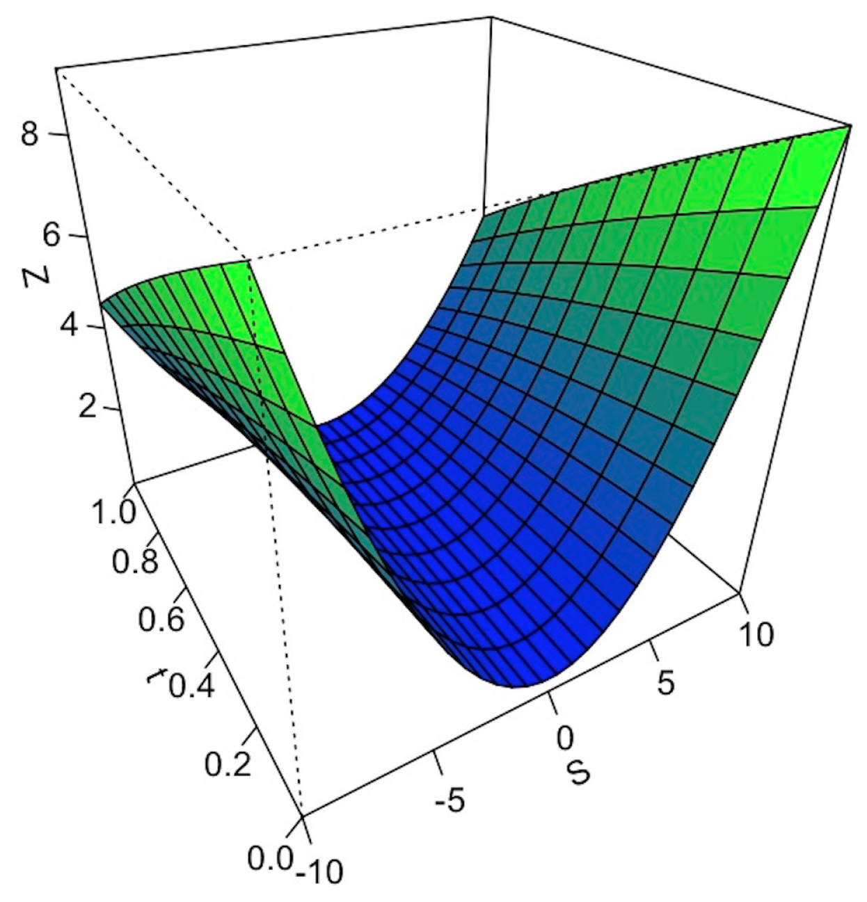
Figure 1. The value function.
Stats 04 00058 g001
Figure 2. The wealth process with the parameters α and c when σ = 1 , r = 0.01 and κ = 0.5 . (a) The wealth process X t * . (b) Optimal investment α t * . (c) Optimal consumption c t * .
Stats 04 00058 g002
Figure 3. The wealth process with the parameters α and c when σ = 5 , r = 4 and κ = 5 . (a) The wealth process X t * . (b) Optimal investment α t * . (c) Optimal consumption c t * .
Stats 04 00058 g003
Figure 4. The wealth process with the parameters α and c when σ = 20 , r = 0.01 and κ = 0.5 with n = 1000 . (a) Wealth process X t * . (b) Optimal investment α t * . (c) Optimal consumption c t * .
Stats 04 00058 g004
Figure 5. The wealth process with the parameters α and c when σ = 0.1 , r = 0.01 and κ = 5 with n = 1000 . (a) The wealth process X t * . (b) Optimal investment α t * . (c) Optimal consumption c t * .
Stats 04 00058 g005
Publisher’s Note: MDPI stays neutral with regard to jurisdictional claims in published maps and institutional affiliations.