Portfolio Management of Copula-Dependent Assets Based on P(Y < X) Reliability Models: Revisiting Frank Copula and Dagum Distributions

Abstract

Modern portfolio theory indicates that portfolio optimization can be carried out based on the mean-variance model, where returns and risk are represented as the average and variance of the historical data of the stock’s returns, respectively. Several studies have been carried out to find better risk proxies, as variance was not that accurate. On the other hand, fewer papers are devoted to better model/characterize returns. In the present paper, we explore the use of the reliability measure $P(Y<X)$ to choose between portfolios with returns given by the distributions X and Y. Thus, instead of comparing the expected values of X and Y, we will explore the metric $P(Y<X)$ as a proxy parameter for return. The dependence between such distributions shall be modelled by copulas. At first, we derive some general results which allows us to split the value of $P(Y<X)$ as the sum of independent and dependent parts, in general, for copula-dependent assets. Then, to further develop our mathematical framework, we chose Frank copula to model the dependency between assets. In the process, we derive a new polynomial representation for Frank copulas. To perform a study case, we considered assets whose returns’ distributions follow Dagum distributions or their transformations. We carried out a parametric analysis, indicating the relative effect of the dependency of return distributions over the reliability index $P(Y<X)$. Finally, we illustrate our methodology by performing a comparison between stock returns, which could be used to build portfolios based on the value of the the reliability index $P(Y<X)$.

1. Introduction

Portfolio management and optimization consist of selecting a set of assets, and their respective portfolio participation weights, which best satisfy the investor’s ideal risk–return relationship [1]. One of the earliest and most important studies in this direction was performed by Markowitz, who proposed the Mean-Variance (MV) model [2]. The author considered that a suitable proxy variable for returns would be the average of the historical data of the stock’s return, and the proxy variable for risk would be the variance of these returns [3].

From the seminal work of Markowitz [2], several researchers studied variations and enhancements of his so-called modern portfolio theory. Normally, studies were carried out to find better risk proxies, as variance was not that accurate. For example, Conditional-Value-at-Risk (CVaR) is proposed by Uryasev [4] as a risk measure of the portfolio, and therefore optimization would be on top of that metric.

Other researchers considered a robust optimization approach, where the uncertainty generated by the errors of estimation of the parameters used in optimization were mathematically accounted for in the model [5]. Several review papers were also devoted to explore Portfolio optimization methods. For example, several authors covered the following topics: Evolutionary computation in the discovery of rules in algorithmic trading for shares [6]; swarm intelligence research for portfolio optimization [7]; portfolio optimization problem with the Markowitz mean-variance structure [3]; 20 years of portfolio optimization based on operational research [8].

Despite these contributions, fewer papers were devoted to better model/characterize returns. In general, researchers were worried about forecasting the returns, but few alternative proxy parameters have been proposed. Literature reveals that classical strategies, such as Markowitz MV portfolio, applied with parameters estimated from data normally provide highly volatile portfolio weights. This is primarily due to the difficulty of estimating expected returns with sufficient accuracy [9,10].

To address this issue, several different methods have been reported in the literature. These methods range from combining Capital Asset Pricing Model (CAPM) equilibrium with subjective investor views to estimate returns [9] to applying the Arbitrage Pricing Theory (APT) [11]. Despite these efforts, the problem of getting unstable portfolio weights was not fully solved [10].

The portfolio optimization approaches which are based on the modern portfolio theory not only suffer from this instability in portfolio weights, but also lack a better description of the dependence structure between assets. Markowitz MV portfolio assumes that the financial returns are subject to a joint normal distribution, implying that the dependence between financial returns is fully described by the linear correlation coefficient [2,12].

Empirical studies indicate that the assumption of normality of financial returns distributions does not hold, indicating the need to examine such distributions by considering extra moments, such as the skewness (the third moment of distribution) and the kurtosis (the fourth moment of distribution) of the real-world returns datasets collected [12].

In order to overcome this shortcoming, several authors studied a number of methods to better characterize the dependence structure of assets’ returns such as: Exceedance correlation [13] and the extreme value theory [14,15,16]; multivariate Generalized Auto Regressive Conditional Heteroskedasticity (GARCH) model with skewness [17] and/or kurtosis [18,19]. These methods are adequate to model time-varying conditional correlations, however they cannot reproduce asymmetries in asymptotic tail dependence [12].

An increasingly applied method to account for such tail dependence is to consider the copula theory, which allows one to model the dependence structure of multivariate data without imposing any assumption on marginal distributions [12]. As pointed out by several authors, the advantage of copula lies in separating marginal distributions and dependence structure from joint distribution [12].

Therefore, in the present paper, we explore the use of the reliability measure $P(Y<X)$ to choose between portfolios with returns given by the distributions X and Y. Thus, instead of comparing the expected values of X and Y, we will explore the metric $P(Y<X)$ as a proxy parameter for return. The dependence between such distributions shall be modelled by copulas.

This paper presents, at first, some general mathematical formulations and theorems which will latter support an empirical exploratory analysis of the portfolio optimization problem. For simplicity, such analysis considered dependence as being modelled by Frank copulas and that asset prices follow distributions from the Dagum family. For more general applications where multi-asset portfolio are considered, highly dimensional problems of portfolio optimization shall be considered and are out of scope of the present effort.

The paper is structured as follows: Section 2 presents some preliminary aspects of the reliability index $P(Y<X)$. Section 3, on the other hand, introduces some concepts related to the copula modelling of dependence between random variables. This section also presents general results concerning the reliability of copula-dependent random variables. In order to illustrate our methodology, Section 4 revisits Frank copula and presents some novel results for the polynomial representation of such copula type. Section 5 then presents the analytical formulas hereby developed to explicitly and exactly obtain the reliability index $P(Y<X)$ when both X and Y follow Dagum-like distributions whose dependence is modeled by a Frank copula. We finally present a parametric study and a real application of portfolio management of stock data in Section 6. Section 7 presents the conclusions of the present paper. The codes developed and used in the present paper are also presented at the end of the paper.

2. Reliability

When modelling the reliability of a given component whose strength is described by a random variable X subjected to stresses modelled by a random variable Y, the component fails if the stress applied to it exceeds the strength, while the component works whenever $Y<X$. Thus, $P(Y<X)$ is a measure of component reliability [20,21].

Apart from the clear application in problems of physics and engineering, this reliability index is also applicable to the areas of quality control, genetics, psychology, and economics [21]. In special, the index $P(Y<X)$ can be used as a proxy parameter to examine the probability of inequality of variables, leading to a measure of the difference between two populations as $P(Y<X)=P(Y-X<0)$.

Both empirical and analytical studies have been carried out to estimate $P(Y<X)$ when X and Y are independent variables belonging to the same univariate family of distributions. The reader may check [20] for a comprehensive account of this topic. Recent contributions include calculating this reliability index for Generalized Pareto distributions [22,23], two-parameter exponential functions [24,25], logistic random variables [26] and generalized logistic distributions [27]. More recently, [28] obtained analytical expressions for the reliability index when both the variables compared were Stable random variables. All these contributions rely on the assumption of independent stress and strength variables.

Even though the independence assumption may be a first approximation, fewer studies were concerned about accounting for the dependence between X and Y when calculating the reliability index [21]. Such dependence may become crucial for applications in finance. For example, when X and Y are disposable household income and consumption, $P(Y<X)$ is a measure of household financial affordability or $P(X<Y)$ measures household financial fragility [29]. Other finance-related applications include excess-of-loss reinsurance models [30] and stock picking [28].

Studies which tried to assess the relationship between X and Y for the evaluation of the reliability index considered bivariate distributions of strength and stress. In this context, a few of the distributions considered are bivariate normal [31], bivariate Pareto [32], bivariate exponential [33], bivariate gamma [34] and bivariate log-normal [35]. A direct shortcoming of this approach is that a bivariate distribution often admits a certain specific form of dependence between margins only and presupposes that both the marginal distributions are of the same type [21].

Copula-based approaches show up as good candidates to better accommodate the dependence structure between the random variables considered [21,29]. The potential of the copula-based approach is clear since a copula function joins margins of any type (parametric and non-parametric distributions) not necessarily belonging to the same family, and captures various forms of dependence (linear, non-linear, tail dependence etc.) [21].

While the idea of relaxing the independence assumption in the stress-strength models may be addressed by involving any family of copulas, in this work we use Frank copulas. We get a closed-form expression for the reliability index by modeling the dependence through Frank copulas when the marginal distributions of stress and strength are chosen as Dagum-like random variables [36]. Frank copula was chosen since it is commonly used in applications and is implemented in most software packages for copula-based modeling [21]. In the next section, we will present some basic formulations linked to the copula modelling of random variables’ dependence.

3. Copulas and Reliability Measures

In short, a two-dimensional copula is a bivariate distribution function whose margins follow Uniform distributions on $(0,1)$. Sklar’s theorem proves how copulas link joint distribution functions to their one-dimensional margins by proving that any bivariate distribution $H(x,y)$ of variables X and Y, with marginal distributions $F\left(x\right)$ and $G\left(y\right)$, can be written as $H(x,y)=C\left(F\right(x),G(y\left)\right)$, where C is a copula. Thus any copula, together with any marginal distribution, allows us to construct a joint distribution [21,37].

Copula families depend, in general, on one or more parameters called association parameters, say $\theta$, related to the degree of dependence between margins. For simplicity, we may represent the copulas as $C_{\theta }$. To further understand the concepts of copulas and their applications, the reader may refer to the monographs in [37,38].

In order to account for the dependence between stress and strength random variables, we calculate the reliability index under the hypothesis that the bivariate distribution of the stress and strength variables is defined by joining the margins $F\left(x\right)$ and $G\left(y\right)$, of any type, through a copula function $C_{\theta }(F\left(x\right),G\left(y\right))$. Moreover, let the joint density function be denoted as $h(x,y)=c_{\theta }(F\left(x\right),G\left(y\right))f\left(x\right)g\left(y\right)$ where $c_{\theta }(F\left(x\right),G\left(y\right))=\frac{{\partial }^2{C}_{\theta }(F\left(x\right),G\left(y\right))}{\partial F\left(x\right)\partial G\left(y\right)}$ is the copula density, and $f\left(x\right)$, $g\left(y\right)$ indicate the marginal density functions.

In this context, the reliability index for dependent random variables $X\ge 0$ and $Y\ge 0$, can be written as [21]:

$${\displaystyle P(Y<X)={\int }_0^{\infty }{\int }_0^x{c}_{\theta }(F\left(x\right),G\left(y\right))f\left(x\right)g\left(y\right)dydx}$$

(1)

We can rewrite Equation (1) by letting $u=F\left(x\right)$ and $v=G\left(y\right)$. Then:

$$\begin{array}{ccc}\hfill P(Y<X)& =& {\displaystyle {\int }_0^1{\int }_0^{G\left(F^{-1}\left(u\right)\right)}{c}_{\theta }(u,v)dvdu}\hfill \\ \hfill & =& {\displaystyle {\int }_0^1\frac{\partial }{\partial u}{C}_{\theta }(u,v){|}_{v=G\left(F^{-1}\left(u\right)\right)}du}\hfill \end{array}$$

(2)

Theorem 1 (Splitting Theorem).

The reliability measure $P(Y<X)$, where the dependency between X and Y is described by any copula model, can always be split into the sum of two parts as:

$$P(Y<X)=R+D_{\theta },$$

(3)

where R is the value of $P(Y<X)$ when both X and Y are independent and $D_{\theta }$ represents the difference between $P(Y<X)$ when both X and Y are dependent and independent.

Proof. 

For any single parameter copula, with parameter $\iota$, let us suppose without loss of generality that when $\iota ={\iota }_{ind}$, this implies independence between the random variables modeled. Thus, let us define the copula density as $d_{\iota }(u,v)$. Whenever $d_{\iota }(u,v)$ is infinitely differentiable with respect to $\iota$ at a real value ${\iota }_{ind}$, the Taylor series expansion of $d_{\iota }(u,v)$ at $\iota ={\iota }_{ind}$ is:

$${\displaystyle d_{\iota }(u,v)=1+\sum _{n=1}^{\infty }\frac{{\partial }^n}{\partial w^n}{d}_w(u,v){|}_{w={\iota }_{ind}}{(\iota -{\iota }_{ind})}^n=1+h(\theta ,u,v)}$$

(4)

The free term in Equation (4) must be 1 as when the random variables are independent, $\iota ={\iota }_{ind}$. By combining Equations (1) and (4) when $c_{\theta }(u,v)=d_{\iota }(u,v)$:

$${\displaystyle P(Y<X)={\int }_0^{\infty }{\int }_0^{x}f\left(x\right)g\left(y\right)dydx+{\int }_0^{\infty }{\int }_0^{x}h(\theta ,F\left(x\right),G\left(y\right))f\left(x\right)g\left(y\right)dydx}$$

(5)

The first term in Equation (5) can be further simplified as:

$${\displaystyle R={\int }_0^{\infty }G\left(x\right)f\left(x\right)dx,}$$

(6)

which is the value of $P(Y<X)$ when when both X and Y are independent [20].

The result for m-parameter copulas is easily obtained by using the Taylor series in several variables. Besides, an alternative proof follows directly from Ruschendorf’s method to represent copulas [39]. □

We can see that Theorem 1 generalizes the results in [21], which only considered the splitting when using the Farlie-Gumbel-Morgenstern and its generalizations. Moreover, we should highlight that, regardless of the type of distribution considered, for any strictly increasing or strictly decreasing continuous function $\beta \left(x\right)$:

$$P(Y<X)=P\left(\beta \right(Y)<\beta (X\left)\right),$$

(7)

which may come in handy when dealing with transformed variables.

4. Revisiting Frank Copula

In order to actually calculate the reliability index for real assets, we need to choose a copula model. As previously indicated, we chose Frank copulas. For this particular type of copula [21,37]:

$$C_{\theta }(u,v)=-\frac{1}{\theta }ln\left(1-\frac{\left(1-e^{-\theta u}\right)\left(1-e^{-\theta v}\right)}{\left(1-e^{-\theta }\right)}\right)$$

(8)

where $\theta \in \mathbb{R}/\left\{0\right\}$. Moreover [21,37]:

$$c_{\theta }(u,v)=\frac{\theta e^{-\theta (u+v)}}{1-e^{-\theta }}{\left(1-\frac{\left(1-e^{-\theta u}\right)\left(1-e^{-\theta v}\right)}{\left(1-e^{-\theta }\right)}\right)}^{-2}$$

(9)

The calculation of the Kendall’s $\tau$ (${\tau }_K$) and Spearman’s $\rho$ (${\rho }_S$) for a Frank copula can be given as [21,37]:

$${\tau }_K=1+4(D{b}_1\left(\theta \right)-1)/\theta$$

(10)

and

$${\rho }_S=12(D{b}_2(-\theta )-D{b}_1(-\theta ))/\theta -1$$

(11)

where $D{b}_k\left(x\right)$ is the Debye function, defined as [21,37]:

$${\displaystyle D{b}_k\left(x\right)=\frac{k}{x^k}{\int }_0^x\frac{t^k}{e^t-1}dt}$$

(12)

In order to find exact representations for the integrals in Equation (2), we first need to obtain the series representation for both $C_{\theta }(u,v)$ and $c_{\theta }(u,v)$. Thus, let one consider the following identities [40]:

$${\displaystyle \frac{x}{e^x-1}=\sum _{n=0}^{\infty }\frac{B_n{x}^n}{n!},\left|x\right|<2\pi }$$

(13)

where $B_n$ is the n-th Bernoulli number. Moreover, the following formula holds as the generating function of Bernoulli polynomials [40]:

$${\displaystyle \frac{x{e}^{xt}}{e^x-1}=\sum _{n=0}^{\infty }\frac{B_n\left(t\right)x^n}{n!},\left|x\right|<2\pi ,t\in \mathbb{R}}$$

(14)

where $B_n\left(t\right)$ is the n-th Bernoulli Polynomial. It is easy to see that $B_n\left(0\right)=B_n$. Besides, another generating function of interest is [41]:

$${\displaystyle exp\left({\displaystyle \sum _{n=1}^{\infty }{\lambda }_n\frac{t^n}{n!}}\right)=1+\sum _{n=1}^{\infty }{Y}_n\left({\lambda }_1,...,{\lambda }_n\right)\frac{t^n}{n!}}$$

(15)

where $Y_n$ is the n-th complete exponential Bell Polynomial. From Bell polynomials theory, the following inversion formula holds [41]:

$${\displaystyle y_n=Y_n\left({\lambda }_1,...,{\lambda }_n\right)=\sum _{k=1}^n{Y}_{n,k}\left({\lambda }_1,...,{\lambda }_{n-k+1}\right)}$$

(16)

where $Y_{n,k}$ is the partial exponential Bell Polynomial [41]. Thus:

$${\displaystyle {\lambda }_n=\sum _{k=1}^n{(-1)}^{k-1}(k-1)!Y_{n,k}\left(y_1,...,y_{n-k+1}\right)}$$

(17)

Let us assume, without loss of generality, that:

$${\displaystyle C_{\theta }(u,v)=\sum _{n=0}^{\infty }{x}_n\frac{{(-\theta )}^n}{n!}}$$

(18)

From Equation (8), one may state that:

$$\frac{\left(1-e^{-\theta u}\right)\left(1-e^{-\theta v}\right)}{\left(1-e^{-\theta }\right)}=1-exp\left({\displaystyle \sum _{n=1}^{\infty }{x}_{n-1}\frac{{(-\theta )}^n}{(n-1)!}}\right)$$

(19)

The Taylor expansion of the exponential function is known as:

$${\displaystyle e^x=\sum _{n=0}^{\infty }\frac{x^n}{n!}}$$

(20)

Thus:

$${\displaystyle \left(1-e^{-\theta u}\right)\left(1-e^{-\theta v}\right)=\sum _{n=1}^{\infty }\frac{{(-\theta u)}^n}{n!}\sum _{n=1}^{\infty }\frac{{(-\theta v)}^n}{n!}}$$

(21)

By performing a change of index in the summations and using the following identity:

$${\displaystyle \sum _{n=0}^{\infty }{a}_n{x}^n\sum _{n=0}^{\infty }{b}_n{x}^n=\sum _{n=0}^{\infty }{c}_n{x}^n,c_n=\sum _{k=0}^n{a}_k{b}_{n-k},}$$

(22)

the product of series in Equation (21) can be given as:

$${\displaystyle \left(1-e^{-\theta u}\right)\left(1-e^{-\theta v}\right)={\theta }^{2}uv\sum _{n=0}^{\infty }\sum _{k=0}^n\frac{u^k{v}^{n-k}}{(k+1)!(n-k+1)!}{(-\theta )}^n}$$

(23)

Thus:

$${\displaystyle \frac{\left(1-e^{-\theta u}\right)\left(1-e^{-\theta v}\right)}{1-e^{-\theta }}=\frac{{\theta }^{2}uv}{1-e^{-\theta }}\sum _{n=0}^{\infty }\sum _{k=0}^n\frac{u^k{v}^{n-k}}{(k+1)!(n-k+1)!}{(-\theta )}^n}$$

(24)

By using the generating function for Bernoulli numbers given in Equation (13), one may get:

$${\displaystyle \frac{\left(1-e^{-\theta u}\right)\left(1-e^{-\theta v}\right)}{1-e^{-\theta }}=\theta uv\sum _{n=0}^{\infty }\frac{B_n}{n!}{(-\theta )}^n\sum _{n=0}^{\infty }\sum _{k=0}^n\frac{u^k{v}^{n-k}}{(k+1)!(n-k+1)!}{(-\theta )}^n,\left|\theta \right|<2\pi }$$

(25)

Equation (25) leads to:

$${\displaystyle \frac{\left(1-e^{-\theta u}\right)\left(1-e^{-\theta v}\right)}{1-e^{-\theta }}=\theta uv\sum _{n=0}^{\infty }\sum _{r=0}^n\sum _{k=0}^r\frac{u^k{v}^{r-k}}{(k+1)!(r-k+1)!}\frac{B_{n-r}}{(n-r)!}{(-\theta )}^n,\left|\theta \right|<2\pi }$$

(26)

From Equations (19) and (15):

$${\displaystyle 1-exp\left({\displaystyle \sum _{n=1}^{\infty }n{x}_{n-1}\frac{{(-\theta )}^n}{n!}}\right)=-\sum _{n=1}^{\infty }{Y}_n\left(x_0,...,n{x}_{n-1}\right)\frac{{(-\theta )}^n}{n!}}$$

(27)

From Equations (27) and (26):

$$\begin{array}{cc}\hfill & {\displaystyle \sum _{n=0}^{\infty }\sum _{r=0}^n\sum _{k=0}^r\frac{u^{k+1}{v}^{r-k+1}}{(k+1)!(r-k+1)!}\frac{B_{n-r}}{(n-r)!}{(-\theta )}^{n+1}}\hfill \\ \hfill =& {\displaystyle \sum _{n=1}^{\infty }\sum _{r=0}^{n-1}\sum _{k=0}^r\frac{u^{k+1}{v}^{r-k+1}}{(k+1)!(r-k+1)!}\frac{B_{n-1-r}}{(n-1-r)!}{(-\theta )}^n}\hfill \\ \hfill =& {\displaystyle \sum _{n=1}^{\infty }{Y}_n\left(x_0,...,n{x}_{n-1}\right)\frac{{(-\theta )}^n}{n!}}\hfill \end{array}$$

(28)

A term by term comparison leads to:

$${\displaystyle Y_n\left(x_0,...,n{x}_{n-1}\right)=n!\sum _{r=0}^{n-1}\sum _{k=0}^r\frac{u^{k+1}{v}^{r-k+1}}{(k+1)!(r-k+1)!}\frac{B_{n-1-r}}{(n-1-r)!}=y_n}$$

(29)

By using the inversion property of Bell Polynomials given in Equations (16) and (17):

$${\displaystyle n{x}_{n-1}=\sum _{k=1}^n{(-1)}^{k-1}(k-1)!Y_{n,k}\left(y_1,...,y_{n-k+1}\right)}$$

(30)

More explicitly:

$$\begin{array}{c}{x}_{n-1}=\hfill \\ \hfill {\displaystyle n^{-1}\sum _{k=1}^n{(-1)}^{k-1}(k-1)!Y_{n,k}\left({\displaystyle uv,...,\sum _{r=0}^{n-k}\sum _{l=0}^r\frac{u^{l+1}{v}^{r-l+1}{B}_{n-k-r}(n-k+1)!}{(l+1)!(r-l+1)!(n-k-r)!}}\right)}\end{array}$$

(31)

The first few terms of the expansion are:

$$\begin{array}{cc}\hfill x_0=& uv\hfill \\ \hfill x_1=& -\frac{uv}{2}(u-1)(v-1)\hfill \\ \hfill x_2=& \frac{uv}{6}\left(2u^2-3u+1\right)\left(2v^2-3v+1\right)\hfill \\ \hfill x_3=& -\frac{uv}{4}(u-1)(v-1)\left(u^2\left(6v^2-6v+1\right)+u\left(-6v^2+6v-1\right)+(v-1)v\right)\hfill \end{array}$$

(32)

Now, we can find the series for $c_{\theta }(u,v)$ given in Equation (9). A first, a direct application of Equation (14) leads to:

$${\displaystyle \frac{\theta e^{-\theta (u+v)}}{1-e^{-\theta }}=\sum _{n=0}^{\infty }\frac{B_n(u+v){(-\theta )}^n}{n!},\left|\theta \right|<2\pi }$$

(33)

On the other hand, Faà di Bruno’s formula states that [41]:

$${\displaystyle \frac{{\partial }^n}{\partial x^n}f\left(g\left(x\right)\right)=\sum _{k=1}^n\frac{{\partial }^k}{\partial y^k}f\left(y\right){|}_{x=g\left(x\right)}{Y}_{n,k}\left(\frac{\partial }{\partial x}g\left(x\right),...,\frac{{\partial }^{n-r+1}}{\partial x^{n-k+1}}g\left(x\right)\right)}$$

(34)

Let:

$${\left(1-\frac{\left(1-e^{-\theta u}\right)\left(1-e^{-\theta v}\right)}{\left(1-e^{-\theta }\right)}\right)}^{-2}=f\left(g\left(\theta \right)\right)$$

(35)

By taking $f\left(y\right)={(1-y)}^{-2}$ and noticing that $g\left(\theta \right)$ has been expressed as a Maclaurin Series of $-\theta$ in Equation (26), it follows that:

$${\displaystyle \frac{{\partial }^n}{\partial x^n}g\left(x\right){|}_{x=0}=-n!\sum _{r=0}^{n-1}\sum _{k=0}^r\frac{u^{k+1}{v}^{r-k+1}}{(k+1)!(r-k+1)!}\frac{B_{n-r-1}}{(n-r-1)!}}$$

(36)

On the other hand,

$$\frac{{\partial }^k}{\partial x^k}f\left(x\right)=(k+1)!{(1-x)}^{-2-k}$$

(37)

Thus:

$${\displaystyle f\left(g\left(\theta \right)\right)=\sum _{n=0}^{\infty }\frac{{(-\theta )}^n}{n!}\frac{{\partial }^n}{\partial x^n}f\left(g\left(x\right)\right){|}_{x=0}}$$

(38)

where:

$${\displaystyle \frac{{\partial }^n}{\partial x^n}f\left(g\left(x\right)\right){|}_{x=0}=\sum _{k=1}^n\frac{{\partial }^k}{\partial y^k}f\left(y\right){|}_{x=g\left(0\right)}{Y}_{n,k}\left(\frac{\partial }{\partial x}g\left(x\right){|}_{x=0},...,\frac{{\partial }^{n-r+1}}{\partial x^{n-k+1}}g\left(x\right){|}_{x=0}\right)}$$

(39)

which is valid for $n\ge 1$. In order to make Equation (39) also valid for $n=0$, in this specific case, it suffices to expand the summation range of k from 1 to ∞ to 0 to ∞. Thus:

$$\begin{array}{cc}\hfill f\left(g\right(\theta \left)\right)=& {\displaystyle \sum _{n=0}^{\infty }\frac{{(-\theta )}^n}{n!}\times }\hfill \\ & {\displaystyle \sum _{k=0}^n(k+1)!Y_{n,k}\left({\displaystyle -uv,...,-\sum _{r=0}^{n-k}\sum _{l=0}^r\frac{u^{l+1}{v}^{r-l+1}{B}_{n-k-r}(n-k+1)!}{(l+1)!(r-l+1)!(n-k-r)!}}\right)}\hfill \end{array}$$

(40)

Finally, from Equations (9), (33) and (40), the following holds:

$$\begin{array}{c}{\displaystyle c_{\theta }(u,v)=\sum _{n=0}^{\infty }\frac{B_n(u+v){(-\theta )}^n}{n!}\sum _{n=0}^{\infty }\frac{{(-\theta )}^n}{n!}\times }\hfill \\ {\displaystyle \sum _{k=0}^n(k+1)!Y_{n,k}\left({\displaystyle -uv,...,-\sum _{r=0}^{n-k}\sum _{l=0}^r\frac{u^{l+1}{v}^{r-l+1}{B}_{n-k-r}(n-k+1)!}{(l+1)!(r-l+1)!(n-k-r)!}}\right),\left|\theta \right|<2\pi }\hfill \end{array}$$

(41)

which can be further simplified as:

$$\begin{array}{c}{\displaystyle c_{\theta }(u,v)=\sum _{n=0}^{\infty }{p}_n{(-\theta )}^n=\sum _{n=0}^{\infty }\sum _{w=0}^n\sum _{k=0}^w\times }\hfill \\ Y_{w,k}\left({\displaystyle -uv,...,-\sum _{r=0}^{w-k}\sum _{l=0}^r\frac{u^{l+1}{v}^{r-l+1}{B}_{w-k-r}(w-k+1)!}{(l+1)!(r-l+1)!(w-k-r)!}}\right)\frac{(k+1)!B_{n-w}(u+v)}{(n-w)!w!}{(-\theta )}^n,\hfill \end{array}$$

(42)

which is valid for $\left|\theta \right|<2\pi$.

The first few terms of the expansion are:

$$\begin{array}{c}{p}_0=1\hfill \\ p_1=-\frac{1}{2}+u+v-2uv\hfill \\ p_2=\frac{1}{12}\left(6u^2-6u+1\right)\left(6v^2-6v+1\right)\hfill \\ p_3=-\frac{1}{12}(2u-1)(2v-1)\left(u^2\left(12v^2-12v+1\right)+u\left(-12v^2+12v-1\right)+(v-1)v\right)\hfill \end{array}$$

(43)

The analytical structure of Frank copulas reveals that this type of copula can be well approximated by polynomial copulas by simply taking as much terms as needed in Equation (42). The series expansions above are valuable to understand the analytical structure of Frank copula models and can be used as approximations when needed.

We can now proceed to obtain exact series representations for the reliability index when Frank copulas are considered.

5. Reliability Calculations

By using the results from Section 4 we can dissect the analytical structure of the equations involved in determining the relative impact of the dependence between X and Y on $P(Y<X)$ when Frank copulas are used to model such dependence.

Moreover, in order to numerically investigate how $P(Y<X)$ changes when the variables compared are dependent, we must choose which distribution the variables involved follow. In this paper, we chose distributions from the Dagum family.

In the present section, the exact expressions for $P(Y<X)$ when both X and Y follow Dagum distributions and have their dependence modelled by Frank copula are presented. These expressions have not been previously obtained in the literature. Moreover, some of the results are obtained in a closed-form in terms of the H-function.

Thus, from Equation (8), it is easy to see that:

$$\frac{\partial }{\partial u}{C}_{\theta }(u,v)=\frac{e^{-\theta u}(1-e^{-\theta v})}{1-e^{-\theta }}{\left(1-\frac{\left(1-e^{-\theta u}\right)\left(1-e^{-\theta v}\right)}{\left(1-e^{-\theta }\right)}\right)}^{-1}$$

(44)

Thus:

$${\displaystyle P(Y<X)={\int }_0^1\frac{e^{-\theta u}(1-e^{-\theta v})}{1-e^{-\theta }}{\left(1-\frac{\left(1-e^{-\theta u}\right)\left(1-e^{-\theta v}\right)}{\left(1-e^{-\theta }\right)}\right)}^{-1}{|}_{v=G\left(F^{-1}\left(u\right)\right)}du}$$

(45)

Now, let $e^{-\theta }=t$, thus:

$${\displaystyle P(Y<X)={\int }_0^1\frac{t^u(1-t^v)}{1-t}{\left(1-\frac{\left(1-t^u\right)\left(1-t^v\right)}{\left(1-t\right)}\right)}^{-1}{|}_{v=G\left(F^{-1}\left(u\right)\right)}du}$$

(46)

When $t<1$ the Binomial expansion leads to:

$$\begin{array}{ccc}\hfill P(Y<X)& =& {\displaystyle {\int }_0^1\frac{t^u(1-t^v)}{1-t}\sum _{n=0}^{\infty }\frac{{\left(1-t^u\right)}^n{\left(1-t^v\right)}^n}{{\left(1-t\right)}^n}{|}_{v=G\left(F^{-1}\left(u\right)\right)}du}\hfill \\ \hfill & =& {\displaystyle \sum _{n=0}^{\infty }{(1-t)}^{-n-1}{\int }_0^1{t}^u{\left(1-t^u\right)}^n{\left(1-t^v\right)}^{n+1}{|}_{v=G\left(F^{-1}\left(u\right)\right)}du}\hfill \end{array}$$

(47)

By using the Binomial expansion again one gets:

$$\begin{array}{c}\hfill \begin{array}{ccc}\hfill P(Y<X)& =& {\displaystyle \sum _{n=0}^{\infty }{(1-t)}^{-n-1}{\int }_0^1{t}^u\sum _{k=0}^n\left(\genfrac{}{}{0pt}{}{n}{k}\right){(-t^u)}^k\sum _{r=0}^{n+1}\left(\genfrac{}{}{0pt}{}{n+1}{r}\right){(-t^v)}^r{|}_{v=G\left(F^{-1}\left(u\right)\right)}du}\hfill \\ \hfill & =& {\displaystyle \sum _{n=0}^{\infty }\sum _{k=0}^n\sum _{r=0}^{n+1}\left(\genfrac{}{}{0pt}{}{n}{k}\right)\left(\genfrac{}{}{0pt}{}{n+1}{r}\right)\frac{{(-1)}^{k+r}}{{(1-t)}^{n+1}}{\int }_0^1{t}^{u(k+1)+vr}{|}_{v=G\left(F^{-1}\left(u\right)\right)}du}\hfill \end{array}\end{array}$$

(48)

By considering the series expansion of the Exponential function:

$$\begin{array}{c}{\displaystyle {\int }_0^1{t}^{u(k+1)+vr}{|}_{v=G\left(F^{-1}\left(u\right)\right)}du={\int }_0^1\sum _{l=0}^{\infty }\frac{{(u(k+1)+vr)}^l{(-\theta )}^l}{l!}{|}_{v=G\left(F^{-1}\left(u\right)\right)}du}\hfill \\ {\displaystyle ={\int }_0^1\sum _{l=0}^{\infty }\frac{{(-\theta )}^l}{l!}\sum _{m=0}^l\left(\genfrac{}{}{0pt}{}{l}{m}\right){\left(u(k+1)\right)}^{l-m}{\left(vr\right)}^m{|}_{v=G\left(F^{-1}\left(u\right)\right)}du}\hfill \\ {\displaystyle ={\sum }_{l=0}^{\infty }\frac{{(-\theta )}^l}{l!}{\sum }_{m=0}^l\left(\genfrac{}{}{0pt}{}{l}{m}\right){(k+1)}^{l-m}{\left(r\right)}^m{\int }_0^1{u}^{l-m}{v}^m{|}_{v=G\left(F^{-1}\left(u\right)\right)}du}\hfill \end{array}$$

(49)

For simplicity, one may define $I_{a,b}\left({\omega }_{X,Y}\right)$ as:

$${\displaystyle I_{a,b}\left({\omega }_{X,Y}\right)={\int }_0^1{u}^a{v}^b{|}_{v=G\left(F^{-1}\left(u\right)\right)}du={\int }_0^1{u}^a{\left(G\left(F^{-1}\left(u\right)\right)\right)}^{b}du}$$

(50)

where ${\omega }_{X,Y}$ represents a vector of parameters which characterize $G\left(F^{-1}\left(u\right)\right)$ and, therefore, X and Y. For simplicity, we may represent $I_{a,b}\left({\omega }_{X,Y}\right)$ as $I_{a,b}$.

From Equations (49) and (50):

$${\displaystyle P(Y<X)=\sum _{n=0}^{\infty }\sum _{k=0}^n\sum _{r=0}^{n+1}\sum _{l=0}^{\infty }\sum _{m=0}^l\left(\genfrac{}{}{0pt}{}{n}{k}\right)\left(\genfrac{}{}{0pt}{}{n+1}{r}\right)\left(\genfrac{}{}{0pt}{}{l}{m}\right)\times \frac{{(-\theta )}^l{(-1)}^{k+r}{(k+1)}^{l-m}{r}^m{I}_{l-m,m}}{{(1-t)}^{n+1}l!}}$$

(51)

which is valid for $\left|\theta \right|<1$.

Equation (51) reveals that the reliability measure $P(Y<X)$ for two random variables whose dependence is described by a Frank copula is fully described by $I_{a,b}$ and $\theta$. Here, $I_{a,b}$ contains all the information about the random variables X and Y, since it depends on the function composition $G\left(F^{-1}\left(u\right)\right)$. From Equations (3) and (50), it can be seen that $I_{0,1}=R$.

To actually calculate the value of the reliability index, we need to choose the marginal distributions. As indicated, we chose Dagum random variables.

Let Z be a continuous random variable taking positive values, $z>0$, whose cummulative distribution function is defined as [36]:

$$F\left(z\right)={(1+{\gamma }_2{z}^{-{\gamma }_3})}^{-{\gamma }_1}$$

(52)

where ${\gamma }_i>0$, $i=1,2,3$ are the distributions parameters. Thus, we say Z is distributed as a Dagum Distribution, $Dag({\gamma }_1,{\gamma }_2,{\gamma }_3)$, and write $Z\sim Dag({\gamma }_1,{\gamma }_2,{\gamma }_3)$.

One can easily obtain the Quantile function for $Z\sim Dag({\gamma }_1,{\gamma }_2,{\gamma }_3)$ as:

$$F^{-1}\left(y\right)={((y^{-1/{\gamma }_1}-1)/{\gamma }_2)}^{-1/{\gamma }_3}$$

(53)

where $0\le y\le 1$.

Thus, if one consider the reliabiliy measure $P(Y<X)$ when $X\sim Dag({\gamma }_{1,1},{\gamma }_{1,2},{\gamma }_{1,3})$ and $Y\sim Dag({\gamma }_{2,1},{\gamma }_{2,2},{\gamma }_{2,3})$, the function $I_{a,b}$ can be calculated as:

$${\displaystyle I_{a,b}={\int }_0^1{u}^a{\left(1+{\gamma }_{2,2}{\left(\frac{u^{-\frac{1}{{\gamma }_{1,1}}}-1}{{\gamma }_{1,2}}\right)}^{\frac{{\gamma }_{2,3}}{{\gamma }_{1,3}}}\right)}^{-b{\gamma }_{2,1}}du}$$

(54)

Literature [42] reveals that:

$${(1+x)}^{-a}=\frac{1}{\Gamma \left(a\right)}{H}_{1,1}^{1,1}\left[x|\begin{array}{c}(1-a,1)\\ (0,1)\end{array}\right]$$

(55)

where $H_{p,q}^{m,n}$ stands for the H-function [42], whose definition is presented in the Appendix A.1. Thus:

$${\displaystyle I_{a,b}={\int }_0^1{u}^a\frac{1}{\Gamma \left(b{\gamma }_{2,1}\right)}{H}_{1,1}^{1,1}\left[{\gamma }_{2,2}{\left(\frac{u^{-\frac{1}{{\gamma }_{1,1}}}-1}{{\gamma }_{1,2}}\right)}^{\frac{{\gamma }_{2,3}}{{\gamma }_{1,3}}}|\begin{array}{c}(1-b{\gamma }_{2,1},1)\\ (0,1)\end{array}\right]du}$$

(56)

By considering the contour representation of the H-function, the following holds [42]:

$$\begin{array}{ccc}{I}_{a,b}\hfill & =& \hfill {\displaystyle \frac{1}{\Gamma \left(b{\gamma }_{2,1}\right)}{\int }_0^1{u}^a\frac{1}{2\pi i}{\int }_L{\left({\gamma }_{2,2}{\left(\frac{u^{-\frac{1}{{\gamma }_{1,1}}}-1}{{\gamma }_{1,2}}\right)}^{\frac{{\gamma }_{2,3}}{{\gamma }_{1,3}}}\right)}^{-s}\Gamma \left(s\right)\Gamma (b{\gamma }_{2,1}-s)dsdu}\\ \hfill & =& \hfill {\displaystyle \frac{1}{\Gamma \left(b{\gamma }_{2,1}\right)\left(2\pi i\right)}{\int }_L{\left(\frac{{\gamma }_{2,2}}{{\gamma }_{1,2}^{\frac{{\gamma }_{2,3}}{{\gamma }_{1,3}}}}\right)}^{-s}\Gamma \left(s\right)\Gamma (b{\gamma }_{2,1}-s){\int }_0^1{u}^a{\left(u^{-\frac{1}{{\gamma }_{1,1}}}-1\right)}^{\frac{-{\gamma }_{2,3}s}{{\gamma }_{1,3}}}duds}\end{array}$$

(57)

In order to calculate the integral in (57), one may notice that:

$${\displaystyle {\int }_0^1{u}^a{\left(u^{-\frac{1}{{\gamma }_{1,1}}}-1\right)}^{\frac{-{\gamma }_{2,3}s}{{\gamma }_{1,3}}}du={\int }_0^1{u}^{a+\frac{{\gamma }_{2,3}s}{{\gamma }_{1,3}{\gamma }_{1,1}}}{\left(1-u^{\frac{1}{{\gamma }_{1,1}}}\right)}^{\frac{-{\gamma }_{2,3}s}{{\gamma }_{1,3}}}du}$$

(58)

By letting $u^{\frac{1}{{\gamma }_{1,1}}}=y$:

$${\displaystyle {\int }_0^1{u}^a{\left(u^{-\frac{1}{{\gamma }_{1,1}}}-1\right)}^{\frac{-{\gamma }_{2,3}s}{{\gamma }_{1,3}}}du={\gamma }_{1,1}{\int }_0^1{y}^{(a+1){\gamma }_{1,1}+\frac{{\gamma }_{2,3}s}{{\gamma }_{1,3}}-1}{\left(1-y\right)}^{\frac{-{\gamma }_{2,3}s}{{\gamma }_{1,3}}}dy}$$

(59)

The Beta function $B(x,y)$ can be defined as [42]:

$$B(x,y)={\int }_0^1{q}^{x-1}{\left(1-q\right)}^{y-1}dq=\frac{\Gamma \left(x\right)\Gamma \left(y\right)}{\Gamma (x+y)}$$

(60)

A direct comparison of Equations (59) and (60) indicates:

$$\begin{array}{ccc}\hfill {\displaystyle {\int }_0^1{u}^a{\left(u^{-\frac{1}{{\gamma }_{1,1}}}-1\right)}^{\frac{-{\gamma }_{2,3}s}{{\gamma }_{1,3}}}du}& =& {\gamma }_{1,1}B\left((a+1){\gamma }_{1,1}+\frac{{\gamma }_{2,3}s}{{\gamma }_{1,3}},1-\frac{{\gamma }_{2,3}s}{{\gamma }_{1,3}}\right)\hfill \\ \hfill & =& \frac{\Gamma \left((a+1){\gamma }_{1,1}+\frac{{\gamma }_{2,3}s}{{\gamma }_{1,3}}\right)\Gamma \left(1-\frac{{\gamma }_{2,3}s}{{\gamma }_{1,3}}\right)}{(a+1)\Gamma \left((a+1){\gamma }_{1,1}\right)}\hfill \end{array}$$

(61)

From Equations (57) and (61):

$$\begin{array}{ccc}\hfill I_{a,b}& =& \frac{1}{\left(2\pi i\right)}{\int }_L{\left(\frac{{\gamma }_{2,2}}{{\gamma }_{1,2}^{\frac{{\gamma }_{2,3}}{{\gamma }_{1,3}}}}\right)}^{-s}\frac{\Gamma \left(s\right)\Gamma (b{\gamma }_{2,1}-s)\Gamma \left((a+1){\gamma }_{1,1}+\frac{{\gamma }_{2,3}s}{{\gamma }_{1,3}}\right)\Gamma \left(1-\frac{{\gamma }_{2,3}s}{{\gamma }_{1,3}}\right)}{(a+1)\Gamma \left(b{\gamma }_{2,1}\right)\Gamma \left((a+1){\gamma }_{1,1}\right)}ds\hfill \\ \hfill & =& \frac{1}{(a+1)\Gamma \left(b{\gamma }_{2,1}\right)\Gamma \left((a+1){\gamma }_{1,1}\right)}{H}_{2,2}^{2,2}\left[\frac{{\gamma }_{2,2}}{{\gamma }_{1,2}^{\frac{{\gamma }_{2,3}}{{\gamma }_{1,3}}}}|\begin{array}{c}(1-b{\gamma }_{2,1},1),\left(0,\frac{{\gamma }_{2,3}}{{\gamma }_{1,3}}\right)\\ (0,1),\left((a+1){\gamma }_{1,1},\frac{{\gamma }_{2,3}}{{\gamma }_{1,3}}\right)\end{array}\right]\hfill \\ \hfill & =& \frac{1}{(a+1)\Gamma \left(b{\gamma }_{2,1}\right)\Gamma \left((a+1){\gamma }_{1,1}\right)}{H}_{2,2}^{2,2}\left[\frac{{\gamma }_{1,2}^{\frac{{\gamma }_{2,3}}{{\gamma }_{1,3}}}}{{\gamma }_{2,2}}|\begin{array}{c}(1,1),\left(1-(a+1){\gamma }_{1,1},\frac{{\gamma }_{2,3}}{{\gamma }_{1,3}}\right)\\ (b{\gamma }_{2,1},1),\left(1,\frac{{\gamma }_{2,3}}{{\gamma }_{1,3}}\right)\end{array}\right]\hfill \end{array}$$

(62)

An interesting case shows up when both X and Y are identically distributed, i.e., ${\gamma }_{1,j}={\gamma }_{2,j}$, $j=1,2,3$ and $G\left(F^{-1}\left(u\right)\right)=u$:

$${\displaystyle P(Y<X)=\sum _{n=0}^{\infty }{(1-t)}^{-n-1}{\int }_0^1{t}^u{\left(1-t^u\right)}^{2n+1}du=-\sum _{n=0}^{\infty }\frac{{(1-t)}^{(n+1)}}{2(n+1)log\left(t\right)}=\frac{1}{2}}$$

(63)

By using the expressions hereby derived, we can illustrate the calculations of the reliability index.

6. Numerical Calculations

From a theoretical point of view, the series obtained in Equation (51) are important to show the analytical structure of the reliability measure $P(Y<X)$ when both X and Y follow Dagum distributions whose dependence is modeled by a Frank Copula.

On the other hand, from a numerical point of view, the series in Equation (51) converges well for $\left|\theta \right|<1$. Around 30 terms are needed on each infinite summation presented in Equation (51) to account for a 4-digit accuracy. The computation, on the other hand, is not fast as it considers nested series with large factorials involved.

For values of $\theta$ outside this range, instead of looking for other series expansions, the integrand in Equation (46) is quite well behaved. Therefore, simple numerical integration techniques can be employed to get high accuracy results.

If we consider the generalized midpoint integration rule, the integral in (46) can represented as:

$$P(Y<X)=\underset{n\to \infty }{lim}\frac{1}{n}\left({\displaystyle \sum _{k=1}^{n-1}\frac{t^{k/m}(1-t^{G\left(F^{-1}(k/m)\right)})}{(1-t)-\left(1-t^{k/m}\right)\left(1-t^{G\left(F^{-1}(k/m)\right)}\right)}+\frac{1}{2}}\right)$$

(64)

where $t=exp(-\theta )$ and:

$$G\left(F^{-1}\left(x\right)\right)={\left(1+{\gamma }_{2,2}{\left(\frac{x^{-\frac{1}{{\gamma }_{1,1}}}-1}{{\gamma }_{1,2}}\right)}^{\frac{{\gamma }_{2,3}}{{\gamma }_{1,3}}}\right)}^{-b{\gamma }_{2,1}}$$

(65)

Numerical experiments show that the summation in Equation (64) provide high accuracy results for n around 200. The computation above is quite fast, as only standard functions are involved and it is valid for all the possible values of $\theta$.

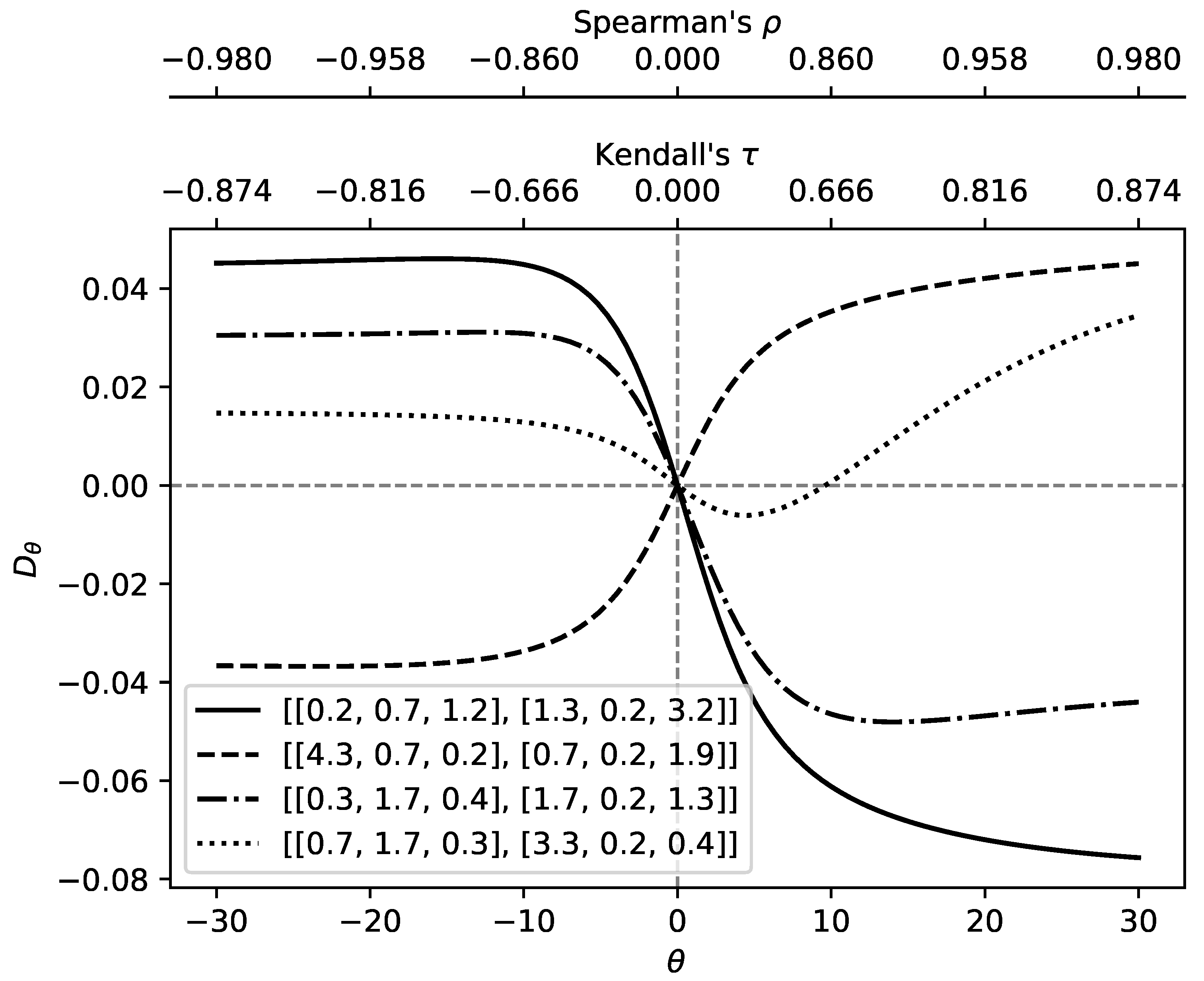
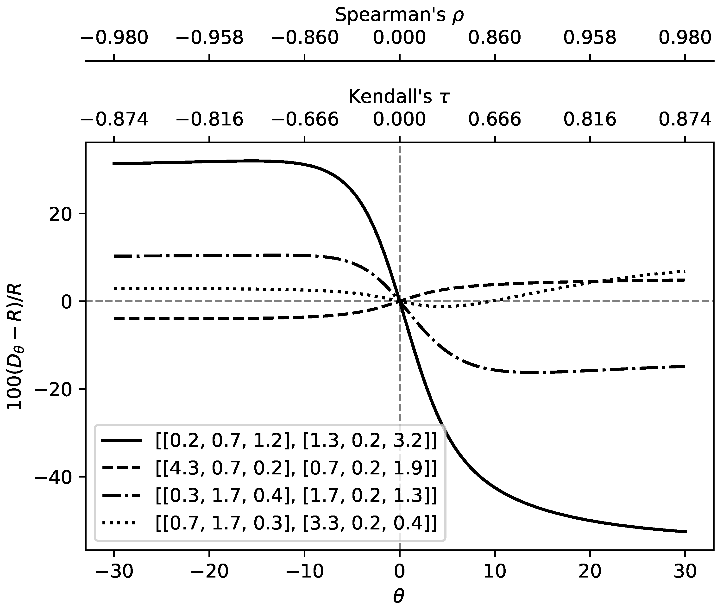
6.1. Parametric Study

Now that the computation requirements have been discussed, one may investigate how $D_{\theta }$ is affected by the parameters of the Dagum random variables modeled as well as the value of $\theta$ for the Frank copula used to model the dependency relation between those RVs. Figure 1 and Figure 2 present some results. Additional horizontal axes, placed on top of the plots, present the correspondent values of Kendall’s $\tau$ and Spearman’s $\rho$ according to the values of $\theta$.

Figure 1 reveals that the impact of $\theta$ on the Reliability measure $P(Y<X)$ is quite important. Since $P(Y<X)$ ranges from 0 to 1, one may see that the impact of the dependence between the random variables can be as high as 0.08 for the variables considered in Figure 1. For high reliability systems, this may be too much.

Figure 2 presents a sense of the relative importance of $D_{\theta }$ with respect to R. It can be seen that $D_{\theta }$ may be almost the half of R for some of the cases studied.

One important aspect to be highlighted from the analysis of Figure 1 and Figure 2 is that the sign of $\theta$ does not always represent the relative impact of $D_{\theta }$ on $P(Y<X)$. Besides, Figure 1 and Figure 2 indicate that there exist inflection points on the curves, which reveals the sign of $D_{\theta }$ may change even when one is dealing with strictly positive or strictly negative correlation cases (the dotted curve highlights this behavior).

6.2. Applications to Real Stock Data

In the previous section, we performed a parametric study on how the reliability index between Dagum Random variables may be affected by the dependency parameter $\theta$ of Frank copulas.

On the other hand, stock returns cannot be modelled as Dagum random variables as they are not strictly positive. By using (7), it is easy to see that by letting $\beta \left(x\right)=ln\left(x\right)$, all the formulas hereby proposed are also applicable to the random variables $ln\left(X\right)$ and $ln\left(Y\right)$, where both X and Y follow Dagum distributions. These transformed random variables are called Log–Dagum distributions and have been studied as alternative models for financial data [43].

In order to show the applicability of the expressions obtained, three real stock return data have been analysed. The stock return data have been collected from Yfinance Python package.

We highlight that the analysis we will carry out is only illustrative of the real portfolio optimization problem, as the multidimensional nature of multi-asset portfolio is hereby reduced to a single-asset portfolio selection. This, on the other hand, is not a major drawback, as the general methodological approach proposed is still valid.

As described, each data set has been modelled as a Log–Dagum random variable and the reliability of the type $P(Y<X)$ has been calculated. This type of reliability index represents a situation in which a given investor has to choose between two stocks [28]. In the case $P(Y<X)<1/2$, the reliability analysis indicates that the random variable Y is more profitable, as its returns are greater than the ones of X. On the other hand, when $P(Y<X)>1/2$ the opposite happens. Finally, when $P(Y<X)=1/2$, there is no difference between both stocks [28].

When using the value of $P(Y<X)$ to build multi-asset portfolios, it is important that such measure satisfy transitivity, i.e., given three distributions X, Y and Z, if $P(X>Y)>0.5$ and $P(Y>Z)>0.5$, we should study if we can infer that $P(X>Z)>0.5$. If a circular ordering among assets X, Y and Z occurs, the optimization procedure of multi-asset portfolios is considerably affected. Proving transitivity of $P(Y<X)$ requires further studies which are out of the scope of the present paper and shall be addressed in future publications. On the other hand, the methodological framework hereby presented is not invalidated. For example, if we consider a finite number of portfolios (which is translated into quantized weights instead of arbitrary weights from 0 to 1), we can perform a brute-force optimization by checking all the possible portfolios. Of course this is not desirable, but can be used as a first approximation.

Python routines have been used to adjust the data to copula-dependent Log–Dagum distributions, to estimate the value of Kendall’s $\tau$ from empirical data and to calculate the reliability index $P(Y<X)$. In special, Kendall’s $\tau$ has been estimate by using the $.corr\left(method{=}^{\prime }kendal{l}^{\prime }\right)$ from Pandas Library. Moreover, the values of the parameters of the fitted Log–Dagum distributions and the respective value of the Frank copula parameter $\theta$ were obtained as Maximum Likelihood Estimates by using a Python code based on the pycopula package. The codes are given in the Appendix A.2.

The stock return data analysed is presented in

Table 1. Stock return data modelled.

Random Variable	Company Code	Company Name
$X_1$	BHP	BHP Group
$X_2$	XOM	Exxon Mobil Corporation
$X_3$	RIO	Rio Tinto Group

and corresponds to the period from 1 January 2010 to 31 December 2020.

Regarding the reliability evaluation, four approaches are used to compare both theoretical and real data. At first, the reliability index $P(Y<X)$ has been estimated from real data by following the procedure [28]:

• Collect the real stock return data samples from 1 January 2010 to 31 December 2020 using the Yfinance Python package for the random variables X and Y;
• Let l be the length of the collected data. Moreover, let $x_i$ and $y_i$, $i=1,...,l$, denote the elements of the real samples of the real variables X and Y, respectively. Consider the indicator function $I(x,y)=1-u(x-y)$, where $u\left(x\right)=0$, $x<0$ and $u\left(x\right)=1$, otherwise. The value of $P(X<Y)$ can be estimated as $P{(X<Y)}_e={\displaystyle \sum _{i=1}^l}I(x_i,y_i)$ and $P(Y<X)$ is simply $1-P(X<Y)$;

For the random variables presented in Table 1, the reliability estimator can be evaluated by following the procedure below [28]:

• Generate random samples with ${10}^5$ elements each for the random variables X and Y;
• Let $x_i$ and $y_i$, $i=1,...,{10}^5$, denote the elements of the random samples of the random variables X and Y, respectively. Consider the indicator function $I(x,y)=1-u(x-y)$, where $u\left(x\right)=0$, $x<0$ and $u\left(x\right)=1$, otherwise. The value of $P(X<Y)$ can be estimated as $P{(X<Y)}_e={\displaystyle \sum _{i=1}^{{10}^5}}I(x_i,y_i)$. Thus, $P(Y<X)$ is simply $1-P(X<Y)$;
• Repeat the above process 1000 times and then take the mean value of the $P{(Y<X)}_e$s generated as the estimated value of $P(Y<X)$. We also compute the standard deviation of such results to check the suitability of the mean estimate.

Finally, Equations (46) and (64) are used to calculate the reliability index for the fitted random variables. In the next subsections, the random variables presented in Table 1 are compared.

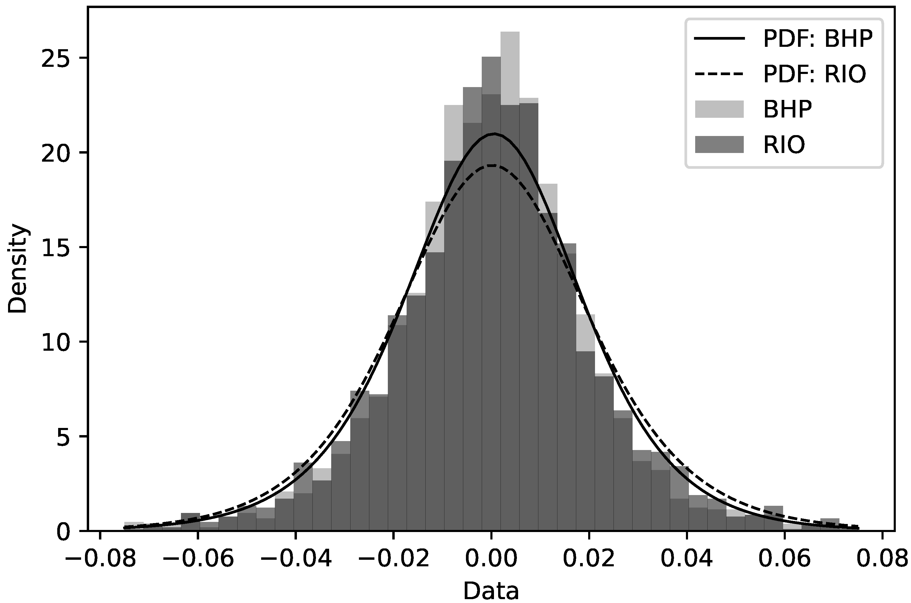
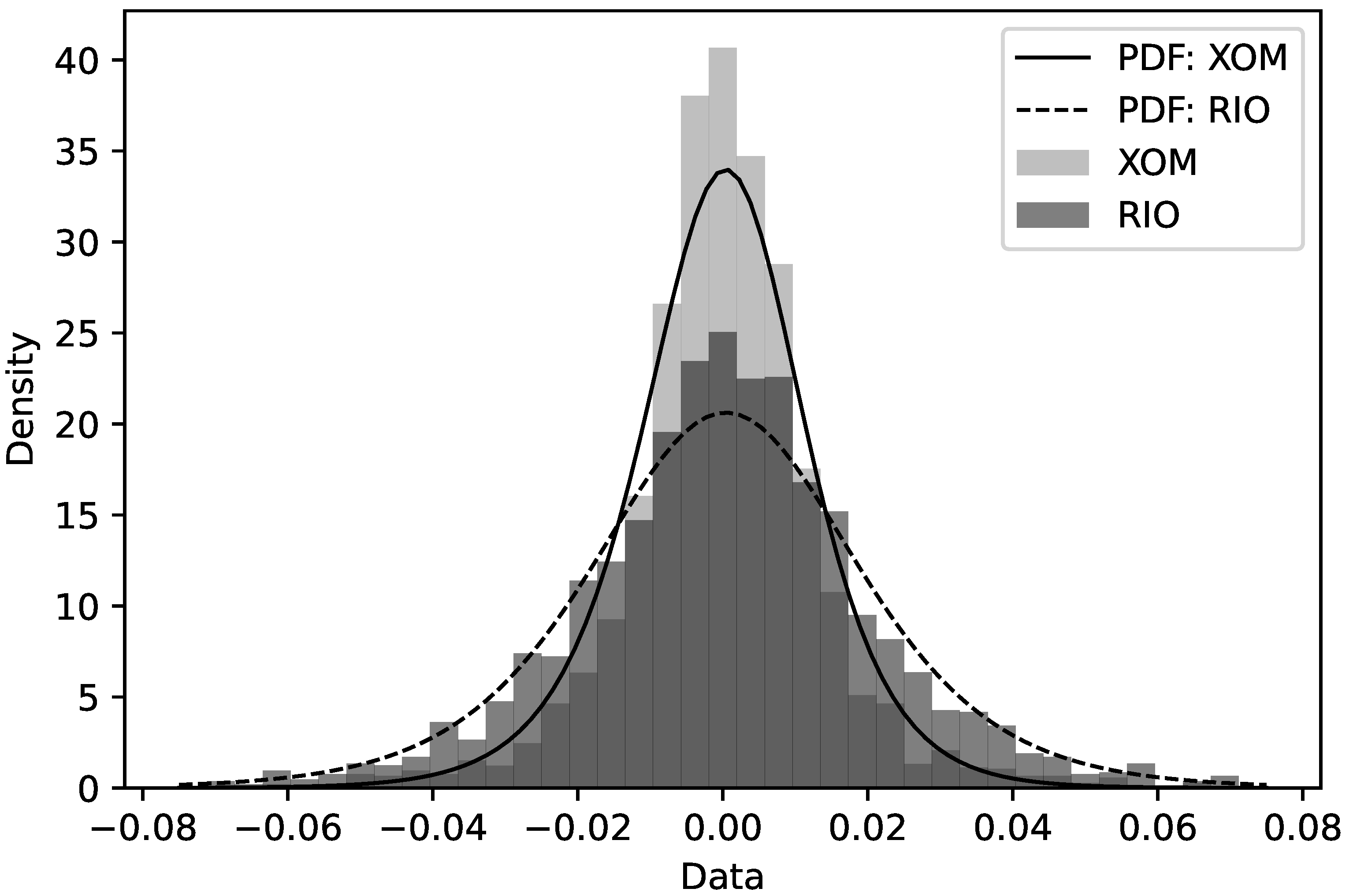
6.2.1. Modelling Stock Return Data as Log–Dagum Random Variables

At first, the Maximum Likelihood Estimates (MLE) of the Log–Dagum distributions’ hyper-parameters and the Frank copulas $\theta$ parameters are given in

Table 2. MLE for $P(X_1<X_3)$.

Random Variables	$\mathit{\theta }$
$X_1\sim LD(0.957,1.092,85.078)$	12.275
$X_3\sim LD(1.032,0.980,76.521)$

and

Table 3. MLE for $P(X_2<X_3)$.

Random Variables	$\mathit{\theta }$
$X_2\sim LD(0.884,1.192,141.362)$	4.182
$X_3\sim LD(0.982,1.054,82.934)$

. It is worth noticing that the pycopula code used maximizes the log-likelihood function over all parameters and hyper-parameters of marginals. Thus, the estimation procedure carried out presents the copula’s parameter and all estimated hyper-parameters at the same time.

Moreover, the initial values of the marginal’s hyper-parameters used in the optimization procedure were the MLE obtained as if the variables were independent. Besides, the initial value of $\theta$ in the optimization algorithm was set to be the Canonical Maximum Likelihood Estimator or $\theta$, obtained by the pycopula package.

Figure 3 and Figure 4 show the real histogram and adjusted p.d.f.s for $X_i$,$i=1,...,3$.

As can be verified from Figure 3 and Figure 4, there is a visual agreement between the real data histograms and the fitted p.d.f.s. Moreover, by using the Scipy Python package, both Spearman’s Rank Correlation and Kendall’s Rank Correlation hypothesis tests indicated the random variables analyzed are dependent. In the next subsection, reliability analyses are carried out.

6.2.2. Reliability Analyses

By following the estimation procedures for $P(Y<X)$ and using the equations developed in the present paper, the reliability indexes for the stock return data modelled are shown in

Table 4. Reliability Measures $P(Y<X)$.

Index	Real Data	Rnd Data	Equation (46)	Equation (64) w/10 Term	Equation (64) w/100 Terms	Equation (64) w/400 Terms
$P(X_1<X_3)$	0.495303	0.494546	0.494523	0.495982	0.494575	0.494528
$P(X_2<X_3)$	0.485549	0.487365	0.487262	0.489479	0.487400	0.487282

.

It can be seen from Table 4 that the real and modelled data behave similarly. The standard deviation of the 1000 estimates of $P{(Y<X)}_e$ was below $2.5\times {10}^{-6}$ for both cases of the random data estimation procedures. Moreover, the applicability of Equation (64) is illustrated. By taking up to 100 terms, the approximate and exact reliability formulas differ by less than 0.00015, which is sufficient for practical applications.

If the random variables were considered as independent, the values for R would be 0.498709 and 0.492342 for $P(X_1<X_3)$ and $P(X_2<X_3)$, respectively. In both cases, the values of $D_{\theta }$ are of −0.004186 and −0.00508, respectively. Even though small, these values are almost 1% of the real reliability index and need to be taken into account to better model the stock behavior.

If we were to choose the stocks solely based on the mean values of the historical returns, we would pick the stock of RIO ($X_3$) as the mean values of returns of BHP ($X_1$), XOM ($X_2$) and RIO ($X_3$) are 0.000319, 0.000073 and 0.000554, respectively. This is the opposite of the conclusion we can draw from comparing the reliability metric, as Table 4 reveals that in both cases we would pick other stock over RIO. This comes from the fact that both $P(X_1<X_3)$ and $P(X_2<X_3)$ are less than 0.5, implying that $X_3$ is not statistically greater than $X_1$ and $X_2$.

7. Conclusions

Using the reliability measure $P(Y<X)$ to assess whether a given component with strength X will be able to support stresses given by the random variable Y is not a new concept. On the other hand, the use of such metric to choose between assets whose returns are X and Y has not been extensively explored in the literature.

In the present paper, we describe a mathematical framework to choose between portfolios with returns given by the distributions X and Y. Instead of comparing the expected values of X and Y, we explored the metric $P(Y<X)$ as a proxy parameter for return. Since real assets show correlation between each other, we modeled such dependence by copulas.

By splitting the value of the reliability measure $P(Y<X)$ as the sum of independent and dependent parts, we are able to understand how correlation impact such measure. Then, to further develop our mathematical framework, we chose Frank copula to model the dependency between assets. Understanding the analytical structure of Frank copulas is important to relate this type of copula to other types presented in the literature. We derive a new polynomial representation for Frank copulas, revealing that such copulas can be well approximated by polynomial copulas by simply taking as much terms as needed in this new representation.

Then, to finish our mathematical derivations, we considered the cases where the marginals follow Dagum distributions or their transformations, since these distributions are powerful models which can account for skewness. Our parametric studies revealed that the impact of Frank copulas parameter $\theta$ on the Reliability measure $P(Y<X)$ is quite important. Since $P(Y<X)$ ranges from 0 to 1, the impact of the dependence between the random variables studied was observed to be be as high as $0.08$. This can completely change the asset selection, specially when $P(Y<X)$ is around 0.5.

By applying our methodology to real-world stock data, we could perform a stock picking procedure by calculating $P(Y<X)$ when both X and Y represent stock returns. We considered the cases where returns follow Log–Dagum distributions. The same procedure can be carried out to compare portfolio of stocks, enabling one to build more general portfolios based on the value of the the reliability index $P(Y<X)$. It is important to highlight that the single-asset stock picking procedure we described is just illustrative of the real multi-asset portfolio optimization problem, which shall be covered in subsequent studies. Moreover, considering the impact on the optimization procedure for multi-asset portfolios, proving that $P(Y<X)$ is transitive is still an open problem which must be further studied.

References

- Milhomem, D.A.; Dantas, M.J.P. Analysis of new approaches used in portfolio optimization: A systematic literature review. Production 2020, 30. [Google Scholar] [CrossRef]
- Markowitz, H. Portfolio Selection. J. Financ. 1952, 7, 77–91. [Google Scholar] [CrossRef]
- Zhang, Y.; Li, X.; Guo, S. Portfolio selection problems with Markowitz’s mean–variance framework: A review of literature. Fuzzy Optim. Decis. Mak. 2017, 17, 125–158. [Google Scholar] [CrossRef]
- Uryasev, S. Conditional value-at-risk: Optimization algorithms and applications. In Proceedings of the IEEE/IAFE/INFORMS 2000 Conference on Computational Intelligence for Financial Engineering (CIFEr) (Cat. No.00TH8520), New York, NY, USA, 28–28 March 2000; pp. 49–57. [Google Scholar] [CrossRef]
- Fabozzi, F.J.; Kolm, P.N.; Pachamanova, D.A.; Focardi, S.M. Robust Portfolio Optimization. J. Portf. Manag. 2007, 33, 40–48. [Google Scholar] [CrossRef]
- Hu, Y.; Liu, K.; Zhang, X.; Su, L.; Ngai, E.; Liu, M. Application of evolutionary computation for rule discovery in stock algorithmic trading: A literature review. Appl. Soft Comput. 2015, 36, 534–551. [Google Scholar] [CrossRef]
- Ertenlice, O.; Kalayci, C.B. A survey of swarm intelligence for portfolio optimization: Algorithms and applications. Swarm Evol. Comput. 2018, 39, 36–52. [Google Scholar] [CrossRef]
- Mansini, R.; Ogryczak, W.; Speranza, M.G. Twenty years of linear programming based portfolio optimization. Eur. J. Oper. Res. 2014, 234, 518–535. [Google Scholar] [CrossRef]
- Black, F.; Litterman, R. Global Portfolio Optimization. Financ. Anal. J. 1992, 48, 28–43. [Google Scholar] [CrossRef]
- Lindberg, C. Portfolio optimization when expected stock returns are determined by exposure to risk. Bernoulli 2009, 15, 464–474. [Google Scholar] [CrossRef]
- Ross, S.A. The arbitrage theory of capital asset pricing. J. Econ. Theory 1976, 13, 341–360. [Google Scholar] [CrossRef]
- Boubaker, H.; Sghaier, N. Portfolio optimization in the presence of dependent financial returns with long memory: A copula based approach. J. Bank. Financ. 2013, 37, 361–377. [Google Scholar] [CrossRef]
- Ang, A.; Chen, J. Asymmetric correlations of equity portfolios. J. Financ. Econ. 2002, 63, 443–494. [Google Scholar] [CrossRef]
- Longin, F.; Solnik, B. Extreme Correlation of International Equity Markets. J. Financ. 2001, 56, 649–676. [Google Scholar] [CrossRef]
- Hartmann, P.; Straetmans, S.; Vries, C.G.d. Asset Market Linkages in Crisis Periods. Rev. Econ. Stat. 2004, 86, 313–326. [Google Scholar] [CrossRef] [Green Version]
- Beine, M.; Cosma, A.; Vermeulen, R. The dark side of global integration: Increasing tail dependence. J. Bank. Financ. 2010, 34, 184–192. [Google Scholar] [CrossRef]
- Harvey, C.R.; Siddique, A. Autoregressive Conditional Skewness. J. Financ. Quant. Anal. 1999, 34, 465–487. [Google Scholar] [CrossRef]
- Jondeau, E.; Rockinger, M. Conditional volatility, skewness, and kurtosis: Existence, persistence, and comovements. J. Econ. Dyn. Control 2003, 27, 1699–1737. [Google Scholar] [CrossRef] [Green Version]
- Brooks, C.; Burke, P.; Heravi, S.; Persand, G. Autoregressive Conditional Kurtosis. J. Financ. Econom. 2005, 3, 399–421. [Google Scholar] [CrossRef] [Green Version]
- Kotz, S.; Lumelskii, Y.; Pensky, M. The Stress-Strength Model and Its Generalizations; World Scientific Publishing Co. Pte Ltd.: Singapore, 2003. [Google Scholar]
- Domma, F.; Giordano, S. A copula-based approach to account for dependence in stress-strength models. Stat. Pap. 2013, 54, 807–826. [Google Scholar] [CrossRef]
- Rezaei, S.; Tahmasbi, R.; Mahmoodi, M. Estimation of P(Y<X) for generalized Pareto distribution. J. Stat. Plan. Inference 2010, 140, 480–494. [Google Scholar] [CrossRef]
- Wong, A. Interval estimation of P(Y<X) for generalized Pareto distribution. J. Stat. Plan. Inference 2012, 142, 601–607. [Google Scholar] [CrossRef]
- Baklizi, A. Estimation of Pr(X<Y) Using Record Values in the One and Two Parameter Exponential Distributions. Commun.-Stat.-Theory Methods 2008, 37, 692–698. [Google Scholar] [CrossRef]
- Sengupta, S. Unbiased estimation of P(X>Y) for two-parameter exponential populations using order statistics. Statistics 2011, 45, 179–188. [Google Scholar] [CrossRef]
- Ozelim, L.C.S.M.; Otiniano, C.E.G.; Rathie, P.N. On The Linear Combination of N Logistic Random Variables and Reliability Analysis. South East Asian J. Math. Math. Sci. 2016, 12, 19–34. [Google Scholar]
- Ozelim, L.C.S.M.; Rathie, P.N. Linear Combination and Reliability of Generalized Logistic Random Variables. Eur. J. Pure Appl. Math. 2019, 12, 722–733. [Google Scholar] [CrossRef]
- Rathie, P.N.; Ozelim, L.C.S.M. Exact and approximate expressions for the reliability of stable Lévy random variables with applications to stock market modelling. J. Comput. Appl. Math. 2017, 321, 314–322. [Google Scholar] [CrossRef]
- Domma, F.; Giordano, S. A stress–strength model with dependent variables to measure household financial fragility. Stat. Methods Appl. 2012, 21, 375–389. [Google Scholar] [CrossRef]
- Embrechts, P.; Kluppelberg, C.; Mikosch, T. Modelling Extremal Events: For Insurance and Finance (Stochastic Modelling and Applied Probability); Springer: Berlin/Heidelberg, Germany, 2008. [Google Scholar]
- Gupta, R.C.; Subramanian, S. Estimation of reliability in a bivariate normal distribution with equal coefficients of variation. Commun. Stat.-Simul. Comput. 1998, 27, 675–698. [Google Scholar] [CrossRef]
- Hanagal, D.D. Note on estimation of reliability under bivariate pareto stress-strength model. Stat. Pap. 1997, 38, 453–459. [Google Scholar] [CrossRef]
- Nadarajah, S.; Kotz, S. Reliability for some bivariate exponential distributions. Math. Probl. Eng. 2006, 2006, 041652. [Google Scholar] [CrossRef] [Green Version]
- Nadarajah, S. Reliability for some bivariate gamma distributions. Math. Probl. Eng. 2005, 2005, 924843. [Google Scholar] [CrossRef] [Green Version]
- Gupta, R.C.; Ghitany, M.E.; Al-Mutairi, D.K. Estimation of reliability from a bivariate log-normal data. J. Stat. Comput. Simul. 2013, 83, 1068–1081. [Google Scholar] [CrossRef]
- Dagum, C. Inequality measures between income distributions with applications. Econometrica 1980, 28, 1791–1803. [Google Scholar] [CrossRef]
- Nelsen, R.B. An Introduction to Copulas, 2nd ed.; Springer Series in Statistics; Springer: Berlin/Heidelberg, Germany, 2006. [Google Scholar]
- Joe, H. Multivariate Models and Multivariate Dependence Concepts (Chapman & Hall CRC Monographs on Statistics & Applied Probability), 1st ed.; Chapman and Hall/CRC: London, UK, 1997. [Google Scholar]
- Ruschendorf, L. Construction of multivariate distributions with given marginals. Ann. Inst. Stat. Math. 1985, 37, 225–233. [Google Scholar] [CrossRef]
- Luke, Y.L. The Special Functions and Their Approximations; Mathematics in Science and Engineering 53-1; Academic Press: Cambridge, MA, USA, 1969; Volume 1. [Google Scholar]
- Comtet, L. Advanced Combinatorics: The Art of Finite and Infinite Expansions; D. Reidel Pub. Co.: Dordrecht, The Netherlands, 1974. [Google Scholar]
- Mathai, A.M.; Haubold, H.J. Special Functions for Applied Scientist; Springer: Berlin/Heidelberg, Germany, 2008. [Google Scholar]
- Domma, F.; Perri, P.F. Some developments on the log–Dagum distribution. Stat. Methods Appl. 2009, 18, 205–220. [Google Scholar] [CrossRef]
- Springer, M.D. The Algebra of Random Variables; John Wiley: Hoboken, NJ, USA, 1979. [Google Scholar]