Robust Variable Selection with Optimality Guarantees for High-Dimensional Logistic Regression

Abstract

High-dimensional classification studies have become widespread across various domains. The large dimensionality, coupled with the possible presence of data contamination, motivates the use of robust, sparse estimation methods to improve model interpretability and ensure the majority of observations agree with the underlying parametric model. In this study, we propose a robust and sparse estimator for logistic regression models, which simultaneously tackles the presence of outliers and/or irrelevant features. Specifically, we propose the use of $L_0$-constraints and mixed-integer conic programming techniques to solve the underlying double combinatorial problem in a framework that allows one to pursue optimality guarantees. We use our proposal to investigate the main drivers of honey bee (Apis mellifera) loss through the annual winter loss survey data collected by the Pennsylvania State Beekeepers Association. Previous studies mainly focused on predictive performance, however our approach produces a more interpretable classification model and provides evidence for several outlying observations within the survey data. We compare our proposal with existing heuristic methods and non-robust procedures, demonstrating its effectiveness. In addition to the application to honey bee loss, we present a simulation study where our proposal outperforms other methods across most performance measures and settings.

1. Introduction

Logistic regression is widely used to solve classification tasks and provides a probabilistic relation between a set of covariates (i.e., features, variables or predictors) and a binary or multi-class response [1,2]. The use of the logistic function can be traced back to the early 19th century, when it was employed to describe population growth [3]. However, despite its popularity, the classical logistic regression framework based on maximum likelihood (ML) estimation can suffer from several drawbacks. In this work, we specifically focus on two key challenges: high dimensionality and data contamination. The large dimensionality might lead to overfitting or even singularity of the estimates if the sample size is smaller than the number of features, and this motivates the use of penalized estimation techniques. Importantly, penalized methods can also promote sparsity of the estimates in order to improve the interpretability of the model [4]. On the other hand, the presence of outliers might disrupt classical and non-robust estimation methods leading to biased estimates and poor predictions. In particular, since the log-odds ratio depends linearly on the set of covariates included in the model, an adversarial contamination of the latter might create bad leverage values that break down ML-based approaches [5]. This motivates the development of robust estimation techniques. Notably, penalized estimation and robustness with respect to the presence of outliers are very closely related topics [6,7,8], and they have recently also been combined for logistic regression settings [9,10].

In this work, we provide a provably optimal approach to perform simultaneous feature selection and estimation, as well as outlier detection and exclusion for logistic regression problems. Here optimality refers to the fact the the global optimum of the underlying “double” combinatorial problem is indeed achievable and, even if the algorithm is stopped before convergence, one can obtain optimality guarantees by monitoring the gap between the best feasible solution and the problem relaxation [11,12]. Specifically, we consider an $L_0$ sparsity assumption on the coefficients [13] and a logistic slippage model for the outlying observations [14]. We further build upon the work in [7] and rely on $L_0$-constraints to detect outlying cases and select relevant features. This requires us to solve a double combinatorial problem, across both the units and the covariates. Importantly, the underlying optimization can be effectively tackled with state-of-the-art mixed-integer conic programming solvers. These target a global optimum and, unlike existing heuristic methods, provide optimality guarantees even if the algorithm is stopped before convergence.

We use our proposal to investigate the main drivers of honey bee (Apis mellifera) loss during winter (overwintering), which represents the most critical part of the year in several areas [15,16,17]. In particular, we use survey data collected by the Pennsylvania State Beekeepers Association, which include information related to honey bee survival, stressors and management practices, as well as bio-climatic indexes, topography and land use information [18]. Previous studies mainly focused on predictive performance and relied on statistical learning tools such as random forest, which capture relevance but not effect signs for each feature, and do not account for the possible impact of outlying cases—making results harder to interpret and potentially less robust. In our analysis, based on a logistic regression model, we are able to exclude redundant features from the fit while accounting for potential data contamination through an estimation approach that simultaneously addresses sparsity and statistical robustness. This provides important insights on the main drivers of honey bee loss during overwintering—such as the exposure to pesticides, as well as the average temperature of the driest quarter and the precipitation level during the warmest quarter. We also show that the data set does indeed contain outlying observations.

The remainder of the paper is organized as follows. Section 2 provides some background on existing penalized and robust estimation methods. Section 3 details our proposal and its algorithmic implementation. This is compared with existing methods through numerical simulations in Section 4. Our analysis of the drivers of honey bee loss is presented in Section 5. Final remarks are provided in Section 6.

2. Background

Let $\mathit{X}={({\mathit{x}}_{\mathbf{1}},\dots ,{\mathit{x}}_{\mathit{n}})}^T\in {\mathbb{R}}^{n\times p}$ be an observed design matrix, and $\mathit{y}\in {\{-1,1\}}^n$ the corresponding set of binary response classes. The two-class logistic regression model assumes that the log-odds ratio is a linear function of the covariates

$$log\left(\frac{Pr(y_i=1|{\mathit{x}}_i)}{1-Pr(y_i=1|{\mathit{x}}_i)}\right)={\mathit{x}}_i^T\mathbf{\beta },$$

(1)

where $\mathbf{\beta }\in {\mathbb{R}}^p$ are the unknown regression parameters (possibly sparse). We also assume the presence of an intercept term, so that $\mathbf{\beta }=\{{\beta }_0,{\beta }_1,\dots ,{\beta }_{p-1}\}$ and $\mathit{X}$ contains only 1’s in the first column. Thus, for any ${\mathit{x}}_i\in {\mathbb{R}}^p$, it follows from (1) that

$$Pr(y_i=1|{\mathit{x}}_i)=\frac{exp({\mathit{x}}_i^T\mathbf{\beta })}{1+exp({\mathit{x}}_i^T\mathbf{\beta })}=\frac{1}{1+exp(-{\mathit{x}}_i^T\mathbf{\beta })}$$

and

$$Pr(y_i=-1|{\mathit{x}}_i)=1-Pr(y_i=1|{\mathit{x}}_i)=\frac{1}{1+exp({\mathit{x}}_i^T\mathbf{\beta })}.$$

Hence, in full generality, the logistic model can be expressed as

$$Pr(y_i|{\mathit{x}}_i)=\frac{1}{1+exp(-y_i{\mathit{x}}_i^T\mathbf{\beta })}.$$

(2)

Assuming that $y_i|{\mathit{x}}_i$, for $i=1,\dots ,n$, follow independent Bernoulli distributions, the likelihood function associated to (2) is

$$L(\mathbf{\beta })=\prod _{i=1}^{n}Pr(y_i=1{|{\mathit{x}}_i)}^{(1+y_i)/2}Pr(y_i=-1{|{\mathit{x}}_i)}^{(1-y_i)/2},$$

which provides the ML estimator

$$\widehat{\mathbf{\beta }}=\underset{\mathbf{\beta }}{arg\; min}\sum _{i=1}^{n}d({\mathit{x}}_i^T\mathbf{\beta },y_i)$$

(3)

where the deviance is defined as

$$d({\mathit{x}}_i^T\mathbf{\beta },y_i)=log\left(1+exp(-y_i{\mathit{x}}_i^T\mathbf{\beta })\right).$$

The optimization problem in (3) is convex, and it admits a unique and finite solution if and only if the points belonging to each class “overlap” to some degree (i.e., the two classes are not linearly separable based on predictors information) [19,20]. Otherwise, there exist infinitely many hyperplanes perfectly separating the data, and the ML estimator is undetermined. Importantly, in this setting, the ML estimator is consistent and asymptotically normal as $n\to \infty$ under weak assumptions [21]. However, unlike ML estimation for linear regression problems, there is no closed-form solution for (3), and iterative methods such as the Newton–Raphson algorithm are commonly employed [22], which can be solved through iteratively reweighted least squares [1,22].

2.1. Penalized Logistic Regression

The ML estimator in (3) does not exist if $p>n$. Moreover, in the presence of strong collinearities in the predictor space, even if $p<n$, the ML estimator might provide unstable estimates or lead to overfitting (i.e., to estimates with low bias and high variance and thus poor predictive power). In order to overcome these limitations, penalized estimation methods based on the $L_2$-penalty have been considered [23,24]. To promote sparse estimates and improve interpretability, several authors also studied the use of the $L_1$-norm [4,25]. Although this class of “soft” penalization methods is computationally very efficient due to convexity, it provides biased estimates. Further approaches combine the $L_1$ and $L_2$-norms in what is known as the elastic net penalty [26]—coupled with an adaptive weighting strategy to regularize the coefficients [27]. Importantly, under suitable assumptions, this guarantees that the resulting estimator satisfies the so-called oracle property, meaning that the probability of selecting the truly active set of covariates (i.e., the ones corresponding to nonzero coefficients) converges to one, and at the same time the coefficient estimates are asymptotically normal with the same means and variance structure as if the set of active features was known a priori [28].

Best subset selection is a traditional “hard” penalization method that approaches the feature selection problem combinatorially [29]. Ideally, one should compare all possible fits of a given size, for all possible sizes—say $1\le k_p\le min(n,p)$. This was long considered unfeasible for problems of realistic size p even in the linear regression setting [22]. Nevertheless, leveraging recent developments in hardware and mixed-integer programming solvers, [30] proposed the use of $L_0$-constraints on $\mathbf{\beta }$ to efficiently and effectively solve the underlying best subset logistic regression problem using mixed-integer nonlinear programming techniques. This extends the approach in [11] for linear regression and relies on the $L_0$ pseudo-norm, which is defined as ${\parallel \mathbf{\beta }\parallel }_0={\sum }_{j}I({\beta }_j\ne 0)$, where $I(·)$ is the indicator function. Notably, oracle properties can be established in this setting under weaker assumptions than other proposals [31].

2.2. Robust Logistic Regression

Outliers may influence the fit, hindering the performance of ML-based estimators and leading to estimation bias and weaker inference [32]. Multiple outliers are particularly problematic and difficult to detect since they can create masking (false negative) and swamping (false positive) effects [33]. Here, as in linear regression, raw (deviance) residuals can be used to build several regression diagnostics [33,34,35]. Different approaches have been introduced to overcome the limitations of classical ML estimation in low-dimensional settings [5]. For instance, a weighted counterpart of ML estimation was proposed in [36] (see also [37]), robust M-estimators were developed in [35], and ref. [38] introduced an additional correction term that provides a robust class of Fisher-consistent M-estimators—see also [39,40] for bounded influence estimators. Furthermore, an adaptive weighted maximum likelihood where the estimator efficiency is calibrated in a data-driven way was considered in [41]. A distributionally robust approach was proposed in [42], which is similar in spirit to the use of robust optimization in [30] where uncertainty sets have to be taken into account.

The logistic slippage model, which closely resembles the mean-shift outlier model for linear regression problems [43], was explicitly considered in [14] and leads to the removal of outliers from the fit. However, since the number and position of outlying cases are generally unknown, one should in principle compare the exclusion of $0\le k_n\le n/2$ points from the fit (if one is willing to assume that less than half of the data are in fact contaminated). Building upon high breakdown point estimators and deletion diagnostics, a forward search procedure based on graphical diagnostic tools that is effective in detecting masked multiple outliers and highlights the influence of individual observations on the fit was developed in [44,45]. This approach is robust, computationally cheap and provides a natural order for the observations according to their agreement with the model.

For high-dimensional settings, the authors in [9] focused on the possible contamination of the y labeling and proposed $L_1$ penalization methods for reducing the influence of outliers and performing feature selection. However, this provides a sub-optimal strategy both for sparse estimation [31] and outlier detection [6]. More recently, the elastic net penalty has been combined with a trimmed loss function which excludes the $k_n$ most influential observations from the fit [10]. This mimics the least trimmed squares (LTS) estimator for linear regression [46], and is equivalent to assuming a logistic slippage model. On the other hand, the trimmed loss function is solved through heuristic methods based on resampling, and the elastic net penalty in use is sub-optimal in terms of feature selection.

3. MIProb: Robust Variable Selection under the Logistic Slippage Model

We consider a two-class logistic regression model affected by data contamination (i.e., outliers) and comprising irrelevant covariates. Specifically, we focus on the logistic slippage model, where the number, position and strength of the outliers are unknown [14,43]. The main idea is to enforce integer constraints on the number of outlying cases and relevant features in order to improve the interpretability of the model and its robustness. Now, we introduce a general formulation that in addition to simultaneous feature selection and outlier detection encompasses an optional ridge penalty, which can be useful to tackle strong collinearity structures [26,30], low signal-to-noise ratio regimes [47] and data perturbations [48]. Thus, we propose to solve the following discrete optimization problem:   

$$\begin{array}{cc}\hfill \left[\widehat{\mathbf{\beta }},\widehat{\mathbf{\varphi }}\right]=\underset{\mathbf{\beta },\mathbf{\varphi }}{arg\; min}& \sum _{i=1}^{n}d({\mathit{x}}_i^T\mathbf{\beta }+{\varphi }_i,y_i)\hfill \end{array}$$

(4)

$$\begin{array}{cc}\hfill \mathrm{s}.\mathrm{t}.& {\parallel \mathbf{\beta }\parallel }_0\le k_p\hfill \end{array}$$

(4a)

$$\begin{array}{cc}\hfill & {\parallel \mathbf{\varphi }\parallel }_0\le k_n\hfill \end{array}$$

(4b)

$$\begin{array}{cc}\hfill & {\parallel \mathbf{\beta }\parallel }_2\le l.\hfill \end{array}$$

(4c)

Due to the (double) combinatorial nature of the problem, the formulation in (4) is computationally daunting [49]. Nevertheless, nowadays it can be solved effectively and at times also efficiently with specialized solvers. Importantly, it relates to the use of a trimmed loss function as in [10], and it extends the work in [7] for sparse linear regression models affected by data contamination in the form of mean-shift outliers. However, here the use of a nonlinear and nonquadratic objective function complicates the matter and requires special attention.

We also note that (4) can be easily extended to model structured data, such as hierarchical or group structures. For instance, in Section 5 we enforce the so-called group sparsity constraints [50] to model categorical features. Moreover, it can be naturally extended to multinomial logistic regression models along lines similar to those in [38].

3.1. Algorithmic Implementation

The optimization problem in (4) can be formulated as a mixed-integer conic program. For simplicity, we first consider only the objective function and the $L_2$ ridge-like penalty. Specifically, including auxiliary variables $t_1,\cdots ,t_n$ and r, the objective (4) and the constraint (4c) can be equivalently reformulated as

$$\begin{array}{cc}\hfill \underset{\mathbf{t},r,\mathbf{\beta }}{min}& \sum _{i=1}^n{t}_i+\lambda r\hfill \end{array}$$

(5)

$$\begin{array}{cc}\hfill \mathrm{s}.\mathrm{t}.& t_i\ge log\left(1+exp\left(-y_i({\mathbf{\beta }}^{\prime }{\mathit{x}}_i+{\varphi }_i)\right)\right)\hfill \end{array}$$

(5a)

$$\begin{array}{cc}\hfill & r\ge {\parallel \mathbf{\beta }\parallel }_2.\hfill \end{array}$$

(5b)

The constraints in (5a) can be expressed using the exponential cone

$$K_{exp}=\left\{(x,y,z)\in {\mathbb{R}}^3:yexp(x/y)\le z\right\},$$

and provide

$$exp\left(-t_i\right)+exp\left(u_i-t_i\right)\le 1$$

where $u_i=-y_i({\mathbf{\beta }}^{\prime }{\mathit{x}}_i+{\varphi }_i)$. Including auxiliary variables $z_{i1}$ and $z_{i2}$ such that $z_{i1}\ge exp\left(u_i-t_i\right)$ and $z_{i2}\ge$$exp\left(-t_i\right)$, it follows that (5a) is equivalent to

$$\left\{\begin{array}{c}\left(u_i-t_i,1,z_{i1}\right)\in K_{\exp }\hfill \\ \left(-t_i,1,z_{i2}\right)\in K_{\exp }\hfill \\ z_{i1}+z_{i2}\le 1.\hfill \end{array}\right.$$

Thus, the proposed mixed-integer conic programming formulation for logistic regression in (4) (denoted MIProb for simplicity), which provides sparse estimates for $\mathbf{\beta }$ and removes outliers through $\mathbf{\varphi }$, is    

$$\begin{array}{cc}\hfill \underset{\mathbf{t},\mathbf{z},r,\mathbf{\beta },{\mathbf{z}}^{\beta },\mathbf{\varphi },{\mathbf{z}}^{\varphi }}{min}& \sum _{i=1}^n{t}_i+\lambda r\hfill \end{array}$$

(6)

$$\begin{array}{cc}\hfill \mathrm{s}.\mathrm{t}.& -{\mathcal{M}}_j^{\beta }{z}_j^{\beta }\le {\beta }_j\le {\mathcal{M}}_j^{\beta }{z}_j^{\beta }\hfill \end{array}$$

(6a)

$$\begin{array}{cc}\hfill & -{\mathcal{M}}_i^{\varphi }{z}_i^{\varphi }\le {\varphi }_i\le {\mathcal{M}}_i^{\varphi }{z}_i^{\varphi }\hfill \end{array}$$

(6b)

$$\begin{array}{cc}\hfill & \sum _{j=1}^p{z}_j^{\beta }\le k_p\hfill \end{array}$$

(6c)

$$\begin{array}{cc}\hfill & \sum _{i=1}^n{z}_i^{\varphi }\le k_n\hfill \\ \hfill & \left(u_i-t_i,1,z_{i1}\right)\in K_{\exp }\hfill \\ \hfill & \left(-t_i,1,z_{i2}\right)\in K_{\exp }\hfill \\ \hfill & z_{i1}+z_{i2}\le 1\hfill \\ \hfill & r\ge {\parallel \mathbf{\beta }\parallel }_2\hfill \\ \hfill & z_j^{\beta }\in \{0,1\},{\beta }_j\in \mathbb{R},j=1,\dots ,p\hfill \\ \hfill & z_i^{\varphi }\in \{0,1\},{\varphi }_i\in \mathbb{R},i=1,\dots ,n.\hfill \end{array}$$

(6d)

The big-$\mathcal{M}$ bounds ${\mathcal{M}}^{\beta }$ and ${\mathcal{M}}^{\varphi }$ in constraints (6a) and (6b) have p and n entries, respectively, which can be tailored for each ${\beta }_j$ and ${\varphi }_i$. These should be wide enough to include the true regression coefficients and zero-out the effects of the true outliers, but not so wide as to substantially increase the computational burden.

For instance, an ensemble method based on existing heuristic and robust procedures to create suitable big-$\mathcal{M}$ bounds was considered in [7]. However, a similar approach is challenging in this framework given a “pool” of openly available robust algorithms is not available for logistic regression models—unlike in linear regression. Here, we simply set large, more conservative bounds to maintain accuracy at the cost of computing time. Extensions of additional heuristics to strengthen these bounds are worth further investigation, but beyond the scope of this work. The $L_0$-norm constraints (6c) and (6d) depend on positive integers $k_p$ and $k_n$, which control the sparsity level for feature selection and the trimming level for outlier detection, respectively. As with any selection procedure, these tuning parameters are key to retain selection and detection accuracy. However, $k_p$ and $k_n$ can be treated differently. For the former, any deviation from the true sparsity level will result in false negatives/positives. For the latter, a common approach [10,45] is to select an inflated trimming amount (i.e., higher than the true level) to avoid masking and swamping effects, and then refine the solution to recover efficiency.

Importantly, in this work we use existing specialized solvers (see Section 4) but the development of a tailored approach could be beneficial. For instance, outer approximation techniques in mixed-integer nonlinear programming with dynamic constraint generation were combined in [30], as well as the use of first-order methods, which reduce the computational burden compared to general-purpose solvers. Extensions of such approaches to this setting are left for future work.

3.2. Additional Details

In order to achieve good estimates it is essential to tune the sparsity level $k_p$ and the trimming level $k_n$, as well as the ridge-like tuning parameter $\lambda$ if present, in a data-driven fashion. For instance, one might consider robust counterparts of information criteria or cross-validation. In our simulation study, we do not include the $L_2$-constraint and, for a given trimming level $k_n$, we use a robust version of the Bayesian information criterion (BIC) similarly to [7]. In symbols, this is $\mathrm{BIC}=k_{p}ln(n-k_n)+{\sum }_{i=1}^{n}d({\mathit{x}}_i^T\widehat{\mathbf{\beta }},y_i)$, where $d({\mathit{x}}_i^T\widehat{\mathbf{\beta }},y_i)$ are the final deviances for a given estimator—recall that deviances corresponding to trimmed points are equal to 0. If an intercept term is included in the model, we force its selection as an active feature. Other tuning procedures such as cross-validation benefit from the use of effective warm-starts to accelerate convergence of the algorithm when solving over several training and testing sets splits—see [7] for additional details.

The breakdown point (BdP) is the largest fraction of contamination that an estimator can tolerate before it might provide completely unreliable estimates [51]. It can be formalized either by replacing good units with outliers or adding outliers to an uncontaminated dataset. Using a unit-replacement approach, it has been shown that one can break down (unpenalized) ML estimation by simply removing units belonging to the overlaps among classes [39,52]. Using unit-addition, the authors in [53] showed that when severe outliers are added to a non-separable dataset, ML estimates do not break down due to “explosion” (to infinity), but they can break down due to “implosion” (to zero). Specifically, the BdP for the ML estimator is equal to ${\epsilon }_{\mathrm{ML}}^{*}=2(p-1)/\{n+2(p-1)\}$ (which is 0% asymptotically), since the estimates can implode to zero, adding $2(p-1)$ appropriately chosen outliers. Thus, unlike in linear regression, here one has to take into account not only the explosion of the estimates, but also their implosion, which is often more difficult to detect.

We leave theoretical derivations concerning our MIProb proposal in (6) to future work. However, we note that MIProb clearly represents a trimmed likelihood estimator as a special case, so in this special case it inherits properties such as the high breakdown point [54,55]. Moreover, these results might be combined with the oracle properties for feature selection described in [31] in order to obtain a logistic version of the robustly strong oracle property introduced in [7].

4. Simulation Study

In this section, we use a simulation study to compare the performance of our proposal with state-of-the-art methods. The simulated data is generated as follows. The first column of the $n\times p$ design matrix $\mathit{X}$ comprises all 1’s (for the model intercept) and we draw the remaining entries of each row independently from a standard $(p-1)$-variate normal distribution $N(\mathbf{0},{\mathit{I}}_{p-1})$. The values of the p-dimensional coefficient vector $\mathbf{\beta }$ comprise $p_0$ non-zero entries (including the intercept) and $p-p_0$ zeros. The response labels $y_i\in \{1,-1\}$, for $i=1,\dots ,n$, are generated from Bernoulli distributions with probabilities $1/(1+e^{-{\mathit{x}}_i^T\mathbf{\beta }})$. Next, without loss of generality, we contaminate the first $n_0$ cases with a logistic slippage model, adding the scalar mean shifts ${\mu }_X$ to the active predictors only (excluding the intercept). In order to generate bad leverage points, we also assign opposite signs to the labels of each contaminated unit: $sign(y_i)=-sign({\mathit{x}}_i^T\mathbf{\beta })$.

The simulation scenarios are defined according to the values of the parameters discussed above. Here, we present results for $p_0=4$ active predictors with ${\beta }_j=3$ (without loss of generality, these correspond to the intercept and the last 3 features), sample size $n=100$, increasing dimension $p=20,50$ (low) and 150 (high), $n_0=5$ contaminated units ( i.e., 5% contamination), and mean shifts ${\mu }_X=10$. Each simulation scenario is replicated q independent times, and random test data, say $({\mathit{y}}^{*},{\mathit{X}}^{*})$, are generated from the same simulation scheme, but without any form of contamination.

Different estimators are compared based on: (i) the mean of the negative log-likelihoods $\mathrm{MNLL}(\widehat{\mathbf{\beta }})=\frac{1}{n}{\sum }_{i=1}^{n}d({{\mathit{x}}^{*\mathit{T}}}_i\widehat{\mathbf{\beta }},y_i^{*})$, i.e., the average of deviances computed on the uncontaminated test set; (ii) the outlier misclassification rate $\mathrm{MR}(\widehat{\mathbf{\beta }})=c/n$, where c counts the points of the uncontaminated test set erroneously labeled as outliers; (iii) estimation accuracy in terms of average mean squared error $\mathrm{MSE}(\widehat{\mathbf{\beta }})=\frac{1}{p}{\sum }_{j=1}^p\mathrm{MSE}({\widehat{\beta }}_j)$, where for each ${\widehat{\beta }}_j$ we decompose $\mathrm{MSE}({\widehat{\beta }}_j)=\frac{1}{q}{\sum }_{i=1}^q{({\widehat{\beta }}_{ji}-{\beta }_j)}^2={({\overline{\beta }}_j-{\beta }_j)}^2+\frac{1}{q}{\sum }_{i=1}^q{({\widehat{\beta }}_{ji}-{\overline{\beta }}_j)}^2$ in squared bias and variance (here ${\overline{\beta }}_j=\frac{1}{q}{\sum }_{i=1}^q{\widehat{\beta }}_{ji}$) (iv) feature selection accuracy, measured by the false positive rate $\mathrm{FPR}(\widehat{\mathbf{\beta }})=\left|\{j\in \{1,\dots ,p\}:{\widehat{\beta }}_j\ne 0\wedge {\beta }_j=0\}\right|/\left|\{j\in \{1,\dots ,p\}:{\beta }_j=0\}\right|$ and the false negative rate $\mathrm{FNR}(\widehat{\mathbf{\beta }})=\left|\{j\in \{1,\dots ,p\}:{\widehat{\beta }}_j=0\wedge {\beta }_j\ne 0\}\right|/\left|\{j\in \{1,\dots ,p\}:{\beta }_j\ne 0\}\right|$; (v) outlier detection accuracy, which is similarly measured by $\mathrm{FPR}(\widehat{\mathbf{\varphi }})$ and $\mathrm{FNR}(\widehat{\mathbf{\varphi }})$.

We use the robust oracle estimator as a benchmark, which is a logistic fit computed only for the active set of features and only on the uncontaminated units (we used our MIP formulation to compute the robust oracle). The following estimators are compared: (a) enetLTS with $\alpha =1$ (i.e., robust Lasso) [10]; (b) MIProb, our robust MIP proposal without a ridge-like constraint (see Section 3); (c) MIP, the non-robust MIP implementation performing only feature selection (i.e., as MIProb but using $k_n=0$); (d) Lasso, the non-robust $L_1$-penalized loss computed through the glmnet package in R [4]. Robust methods trim the true number of outliers ($k_n=n_0$), though this does not guarantee exact outlier detection, and only the sparsity level in the feature space is tuned for each method based on (robust) information criteria or cross-validation. However, since enetLTS is a heuristic method that relies on resampling rather than exact trimming, we inflate the trimming proportion to 20% and then take the re-weighted estimates in order to improve its outlier detection performance.

Table 1. Median (MAD in parenthesis) of MNLL, misclassification rate, variance and squared bias for $\widehat{\mathbf{\beta }}$, false positive rate and false negative rate for feature selection and outlier detection based on 30 simulation replicates.

n	p	Method	MNLL	MR	$\mathbf{var}(\widehat{\mathit{\beta }})$	$\mathbf{bias}{(\widehat{\mathit{\beta }})}^2$	$\mathbf{FPR}(\widehat{\mathit{\beta }})$	$\mathbf{FNR}(\widehat{\mathit{\beta }})$	$\mathbf{FPR}(\widehat{\mathit{\varphi }})$	$\mathbf{FNR}(\widehat{\mathit{\varphi }})$
100	20	Oracle	0.24(0.08)	0.11(0.04)	0.85(0.00)	0.29(0.00)	0.00(0.00)	0.00(0.00)	0.00(0.00)	0.00(0.00)
		enetLTS	0.50(0.08)	0.28(0.06)	0.03(0.00)	1.11(0.00)	0.18(0.09)	0.00(0.00)	0.005(0.008)	0.00(0.00)
		MIProb	0.27(0.04)	0.11(0.04)	0.01(0.00)	0.46(0.00)	0.00(0.00)	0.00(0.00)	0.00(0.00)	0.00(0.00)
		MIP	0.64(0.07)	0.31(0.04)	0.02(0.00)	1.52(0.00)	0.06(0.09)	0.75(0.00)	0.00(0.00)	1.00(0.00)
		Lasso	0.62(0.03)	0.29(0.04)	0.005(0.00)	1.52(0.00)	0.00(0.00)	0.75(0.00)	0.00(0.00)	1.00(0.00)
100	50	Oracle	0.22(0.04)	0.09(0.03)	0.10(0.00)	0.02(0.00)	0.00(0.00)	0.00(0.00)	0.00(0.00)	0.00(0.00)
		enetLTS	0.51(0.10)	0.27(0.13)	0.02(0.00)	0.45(0.00)	0.12(0.06)	0.00(0.00)	0.00(0.00)	0.00(0.00)
		MIProb	0.26(0.04)	0.10(0.02)	0.01(0.00)	0.19(0.00)	0.00(0.00)	0.00(0.00)	0.00(0.00)	0.00(0.00)
		MIP	0.69(0.09)	0.37(0.06)	0.02(0.00)	0.63(0.00)	0.04(0.03)	0.75(0.00)	0.00(0.00)	1.00(0.00)
		Lasso	0.62(0.02)	0.29(0.03)	0.002(0.00)	0.63(0.00)	0.00(0.00)	0.75(0.00)	0.00(0.00)	1.00(0.00)
100	150	Oracle	0.21(0.05)	0.09(0.03)	0.07(0.00)	0.02(0.00)	0.00(0.00)	0.00(0.00)	0.00(0.00)	0.00(0.00)
		enetLTS	0.54(0.07)	0.29(0.03)	0.007(0.00)	0.16(0.00)	0.06(0.02)	0.00(0.00)	0.00(0.00)	0.00(0.00)
		MIProb	0.34(0.12)	0.16(0.06)	0.03(0.00)	0.08(0.00)	0.00(0.00)	0.25(0.37)	0.00(0.00)	0.00(0.00)
		MIP	0.88(0.12)	0.42(0.03)	0.02(0.00)	0.21(0.00)	0.03(0.00)	0.75(0.00)	0.00(0.00)	1.00(0.00)
		Lasso	0.62(0.05)	0.30(0.06)	0.002(0.00)	0.21(0.00)	0.007(0.01)	0.75(0.00)	0.00(0.00)	1.00(0.00)

provides medians and median absolute deviations (MAD) of simulation results over $q=30$ replications. Our proposal substantially outperforms competing methods in most criteria. In both low ($p=20,50$) and high ($p=150$) dimensional settings, the MNLL and MR of MIProb are closest to values produced by the oracle. In terms of estimation accuracy, MIProb has the lowest bias, but the non-robust Lasso has distinctly lower variance than all procedures aside from enetLTS when $p=150$. MIProb has very strong feature selection accuracy with FPR$(\widehat{\beta })$ and FNR$(\widehat{\beta })$ equal to 0 in the low-dimensional settings ($p=20,50$). In the high-dimensional setting, it maintains the lowest false positive rate, but has a higher false negative rate than enetLTS (though still lower than the non-robust methods). This motivates the development of more effective tuning strategies as p increases. On the other hand, enetLTS tends to overselect, since it has FNR$(\widehat{\beta })=0$ in all settings, but the highest FPR$(\widehat{\beta })$ across methods. Similar results were found in [7]. Regarding outlier detection, enetLTS and MIProb produce very similar solutions with FPR and FNR almost always 0. Thus, both methods are highly effective at detecting contaminated units.

Computational Details

In this section, we discuss further computational details and the tuning approaches for each procedure. Our proposal, MIProb is computationally more demanding than the other methods under comparison, including the non-robust MIP. This is natural, given methods like enetLTS are heuristics and avoid directly solving the full combinatorial problem. As discussed in more detail in [11,56], a common challenge with MIP formulations is the weak lower bound produced by the relaxed version of the problem. Thus, while the optimal solution may have already been found, the majority of computing time may be used to verify its optimality. For our settings, we set generous stopping criteria where the algorithm ends when either a maximum computing time of 40 min (this can be as low as 3 min in other literature [47]) or an optimality gap of 2.5% (i.e., the relative difference between the upper and lower bounds) is met. While this maximum time may be hit, especially under the most challenging scenarios with $p=150$, the consistent quality of solutions close to the oracle (see Table 1) further supports this observation of weak lower bounds. However, for comparison, enetLTS only takes an average of  14 s. Thus, the use of other warm-starts, heuristics, etc., to improve lower bounds would be very beneficial for MIP-based feature selection and outlier detection approaches.

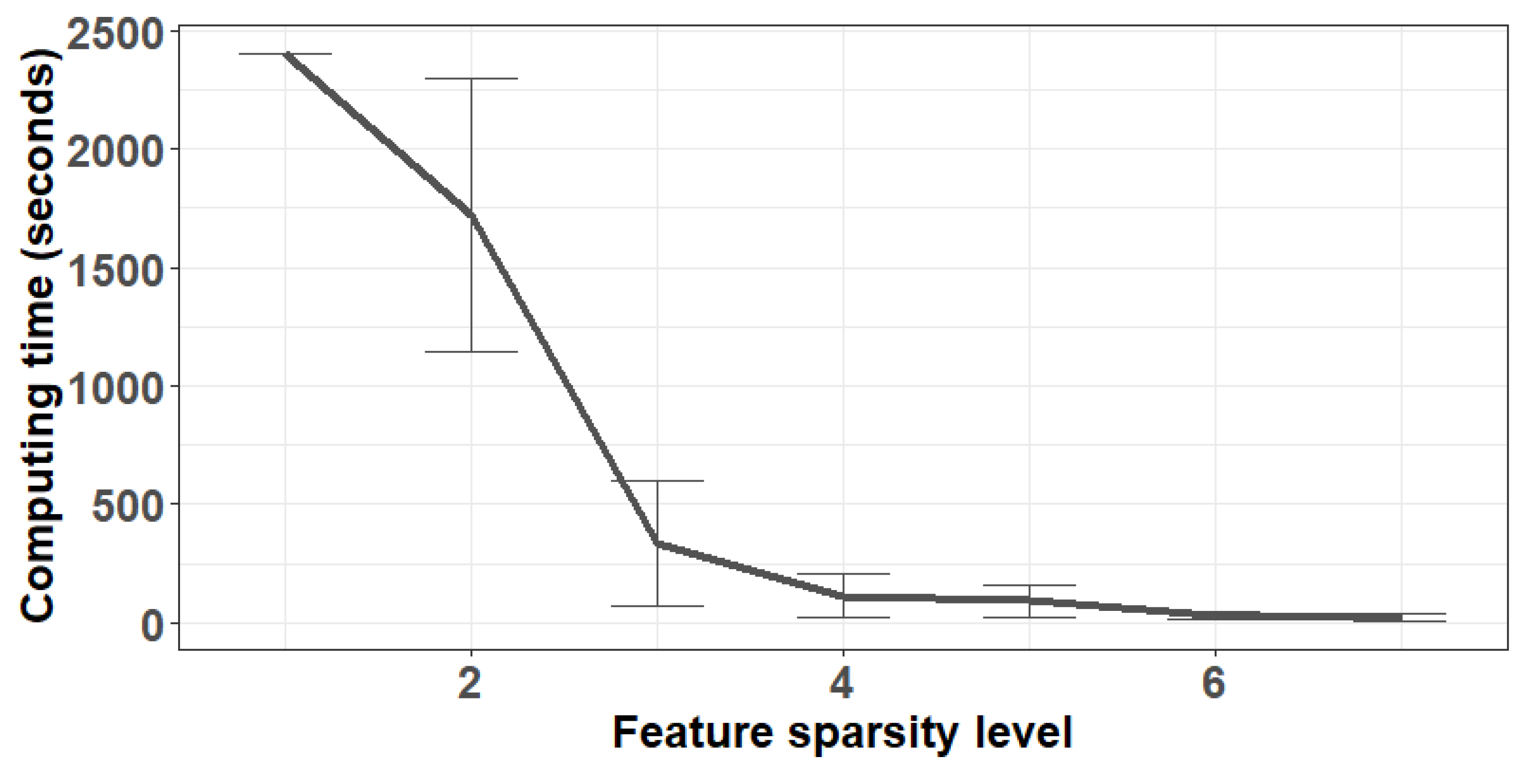
We also found that the computational burden of MIProb varies vastly based on the tuning parameter $k_p$. In our numerical experiments, computing time decreases as more features are selected, especially for $k_p>p_0$. For instance, we considered other simulation scenarios not reported here, including one with a lower sample size $n=50$ and thus a higher contamination percentage. We observed the pattern in Figure 1 where the average computing time is much higher for lower values of $k_p$, but rapidly decreasing after the “elbow” occurring around $k_p=p_0$. This could be due to the outlier detection portion of the problem being more difficult when some of the relevant features are not included. Recall that our simulations add mean shift contamination only to the relevant features; when some are missing, it is more challenging to detect contaminated units.

Regarding tuning, we utilized different approaches for each procedure as appropriate. The oracle operates on uncontaminated units and relevant features only, and requires no tuning. EnetLTS is tuned with cross-validation through the enetLTS package in R following the default settings with 5 folds [57]. For our proposal, MIProb, we used a robust version of BIC as described in Section 3.2, selecting the $k_p$ corresponding to the minimum. Similarly, MIP is tuned based on the traditional BIC (without trimming incorporated). Finally, the non-robust Lasso is tuned through 10-fold cross-validation in the glmnet package. We note that MIProb and MIP are implemented in Julia 1.3.1 to interact with the Mosek solver through its JuMP package. MIProb and enetLTS utilize 24 cores per replication through their multi-thread options.

5. Investigating Overwintering Honey Bee Loss in Pennsylvania

Pollinators play a vital role supporting critical natural and agricultural ecosystem functions. Specifically, honey bees (Apis mellifera) are of great economic importance and play a primary role in pollination services [58,59]. The added value of honey bees pollination for the crops produced in the United States (in terms of higher yield and quality of the product) is annually estimated around 15–20 billion dollars [58,60], and according to the Pennsylvania Beekeepers Association, their yearly contribution has an estimated value of 60 million dollars in the state of Pennsylvania alone; see https://pastatebeekeepers.org/pdf/ValueofhoneybeesinPA3.pdf (accessed on 15 July 2021). Yet the decline of the honey bee populations is a widespread phenomenon around the globe [61,62,63,64,65]. Major threats for honey bees include habitat fragmentation and loss, mites [66,67], parasites and diseases [68], pesticides [69], climate change [70], extreme weather conditions, the introduction of alien species [71], as well as the interactions between these factor [72]. Moreover, the overwintering period is often a major contributor to honey bee loss [15,16,73,74]. We thus focus on honey bee winter survival.

In the United States, beekeepers suffered an average 45.5% overwinter colony loss between 2020 and 2021 [75]. This figure was 41.2% in the state of Pennsylvania for the same overwintering period; see https://beeinformed.org/2021/06/21/united-states-honey-bee-colony-losses-2020-2021-preliminary-results/ (accessed on 15 July 2021). In both cases, this was an increase compared to the previous year, when the reported losses were 43.7% and 36.6% for the United States and Pennsylvania, respectively [76]. In recent years the trend of overwintering loss for Pennsylvania is comparable to the one at the national level, making it an interesting case study. Thus, in the following we analyze overwintering survey data for Pennsylvania covering the years 2016–2019.

5.1. Model Formulation and Data

Focusing on the state of Pennsylvania, honey bee winter survival was recently investigated in [18] based on winter loss survey data provided by the Pennsylvania State Beekeepers Association. The data cover three winter periods (2016–2017, 2017–2018, and 2018–2019), and the main goals of the analysis were to assess the importance of weather, topography, land use, and management factors on overwintering mortality, and to predict survival given current weather conditions and projected changes in climate. The authors utilized a random forest classifier to model overwintering survival. Importantly, they also controlled for the treatment of varroa mites (Varroa destructor) at both apiary and colony levels, since this represents a key factor in describing honey bee survival—all untreated colonies were excluded from the dataset. Their main findings suggest that growing degree days (see

Table 2. Description of the features included in our logistic model formulation to describe honey bee overwintering survival. See [18] for details. The bioc# variables refer to bioclimatic variables of the WorldClim database; see https://www.worldclim.org/data/bioclim.html (accessed on 15 July 2021).

	Variable	Description
1	survival	Binary survival response at the apiary level
2	bee2	Winter total precipitation
3	bee4	Winter days with maximum temperature above 16 °C and precipitation below 3 mm
4	gdd	Growing degree days (base 5 °C) as the accumulation of average daily temperatures
5	dd rain	Days between rain events > 0.25 mm
6	bioc02	Mean diurnal temperature range
7	bioc04	Temperature seasonality
8	bioc08	Mean temperature of the wettest Quarter
9	bioc09	Mean temperature of the driest quarter
10	bioc18	Precipitation of the warmest quarter
11	bioc19	Precipitation of the coldest quarter
12	slope	Terrain slope
13	sol rad	Potential incident solar radiation, 21 December
14	pcurv	Profile curvature
15	tcurv	Terrain curvature
16	TWI	Topographic wetness index
17	EW	East/West orientation of slope
18	ITL	Distance-weighted insect toxic load
19	col nov	Number of colonies in November
20	exp 1–2	Beekeeper years of experience between 1 and 2 (binary variable)
21	exp 2–5	Beekeeper years of experience between 2 and 5 (binary variable)
22	exp < 1	Beekeeper years of experience less than 1 (binary variable)
23	exp > 10	Beekeeper years of experience greater than 10 (binary variable)

) and precipitations in the warmest quarter of the preceding year were the most important predictors, followed by precipitations in the wettest quarter, as well as maximum temperature in the warmest month. These results highlight the strong association between weather events and overwintering survival of honey bees.

The data set used in our analysis is extracted from the Supplementary Information published in [18]—see Table 2 for a description of the variables included into our model.

Since observations in the original data set represent colonies that may belong to the same apiary, we aggregated the data to obtain unique apiary information. This is particularly important in order to reduce dependence across observations, and leads to a sample of $n=257$ apiaries from 1429 colonies (in the absence of publicly available geo-localized information, apiary identification was made possible through the features “bioc02” and “slope”).

We created a binary response taking the proportion of survived colonies per apiary, and assigning the label 1 if such a mean is greater than 0.8, and the label −1 if it is smaller than 0.6. These thresholds are motivated by the “average” winter colony loss rate described above and they allow us to study the most “extreme” behavior (significantly higher or lower losses); they also provide a balanced labeling for the response variable. The remaining observations are completely removed from the data set in use and thus decreasing the sample size to $n=216$.

We compared the same procedures considered in our simulation study (see Section 4) without introducing a ridge-like penalty for any of the methods. Relatedly, we did not use all features in the original study, which presented sizable collinearities. In particular, for each pair of features with an absolute pair-wise correlation above 0.7, we computed the mean absolute correlation of each feature against all the others and removed the one with the largest mean absolute correlation from our pool.

Each column of the design matrix $\mathit{X}$ (excluding the intercept and categorical factors) was standardized to have zero median and median absolute deviation (MAD) equal to the average MAD across columns (standardization does not affect our proposal and each of the other approaches included in our comparison performs its own standardization as needed). Importantly, for MIP and MIProb we introduced group sparsity constraints [50] to tackle the categorical feature “beekeepers’ experience”; the reference category is “between 5 and 10 years” and all coefficients for the dummy variables are included or excluded from the fit together.

5.2. Results

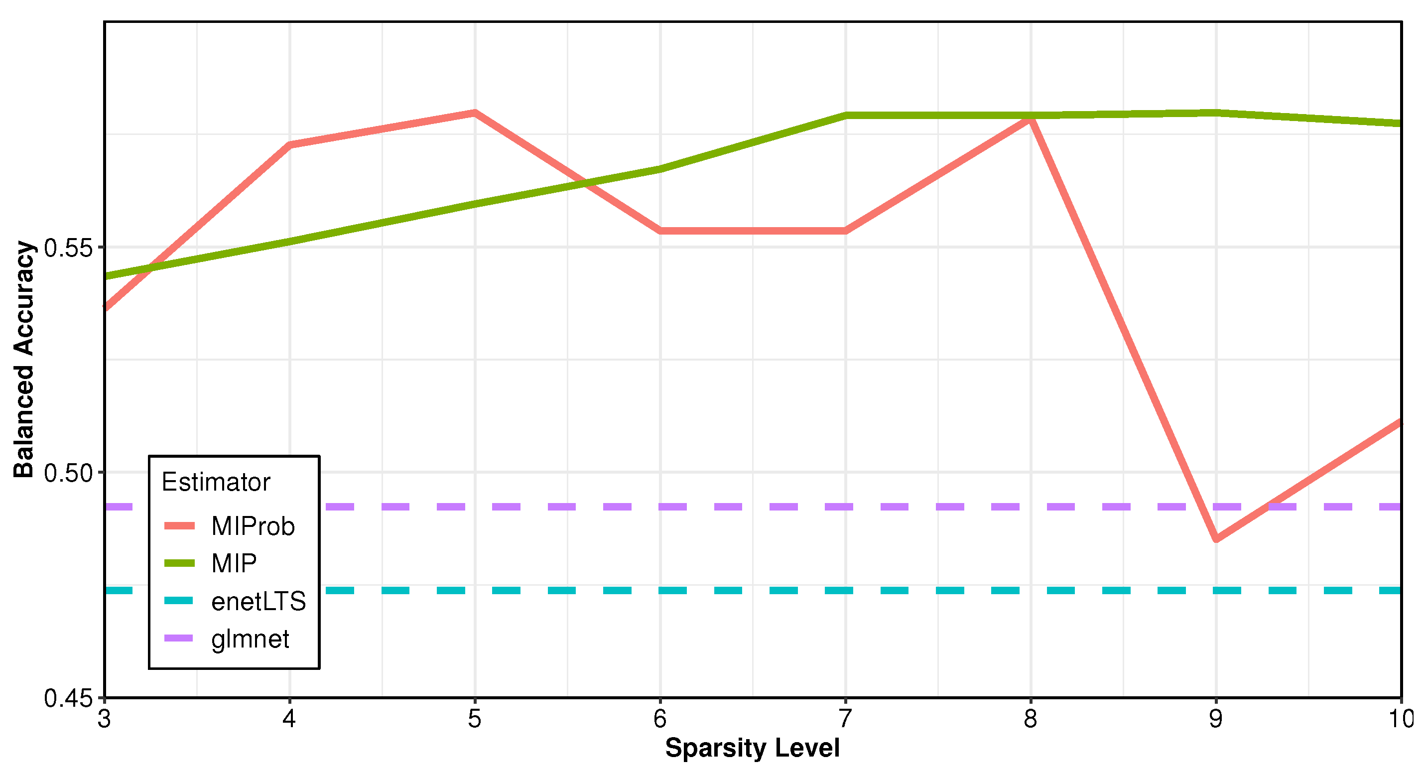
We randomly split the data into training and test sets, encompassing 100 and 116 points, respectively. For robust methods, we fix the trimming proportion at 10% after exploring a range of values suitable for the nature of the problem, and only tune the sparsity level. Figure 2 compares the balanced accuracy, defined as (sensitivity+specificity)/2, on the test set across different methods Here sensitivity is defined as (# true positives)/(# true positives + # true negatives) and specificity is defined as (# true negatives)/(# true negatives + # false positives). While this is a function of the sparsity level imposed on MIP and MIProb, for enetLTS and Lasso we show the mean values across eight repetitions due to the intrinsic randomness induced by cross-validation methods (horizontal dashed lines). Here MIP and MIProb are quite comparable and generally outperform competing methods, although we notice a drop in predictive performance for MIProb if the sparsity level $k_p\ge 9$—which is likely a result of overfitting due to data trimming compared to MIP. Based on these findings, in the following we present the results based on $k_p=8$ (including the intercept), where the balanced accuracy for both methods is very close to their maximum.

Table 3. Features selected by Lasso, MIP, enetLTS and MIProb (robust MIP) on a training set encompassing 100 points. Green and red cells indicate estimated coefficients with positive and negative signs, respectively. White cells indicate non-selected features.

	interc.	bee2	bee4	gdd	dd rain	bioc02	bioc04	bioc08	bioc09	bioc18	bioc19	slope
Lasso
MIP
enetLTS
MIProb
	sol rad	pcurv	tcurv	TWI	EW	ITL	col nov	exp 1–2	exp 2–5	exp < 1	exp > 10
Lasso
MIP
enetLTS
MIProb

displays the features selected by each method on the training set. We focus on the interpretation of the signs of the estimated coefficients, represented as green (positive) and red (negative) cells, respectively. The estimates provided by MIProb are in line with the findings of the original study [18]. Specifically, MIProb estimates a positive association between honey bee survival and “bee2” (winter total precipitation), “gdd” (growing degree days), “EW” (East/West orientation of slope) and “ITL” (distance-weighted insect toxic load, see [77]). This suggests that the impact of precipitations and the accumulation of average daily temperatures (gdd), which influence the growth of crops, have an overall positive effect on honey bee survival. In contrast, MIProb estimates a negative association between honey bee survival and “bioc09” (mean temperature of the driest quarter), “bioc18” (precipitation of the warmest quarter), “tcurv” (terrain curvature) and “TWI” (topographic wetness index). This highlights once more the major impact of weather predictors, as well as topographic factors and humidity levels. Notably, beekeepers’ experience was not selected as a relevant feature by MIProb, which further supports the findings in [18].

Considering the other procedures, enetLTS appears to produce denser solutions (this was also observed in the simulations in Section 4), excluding only three features from the fit, and the non-robust Lasso appears to produce sparser solutions, selecting only three features—which is indeed due to the presence of outliers. This is supported by the fact that a Lasso fit after the exclusion of the outliers detected by MIProb provides richer solutions, corresponding to clearer minima of the cross-validation error, where approximately 10 features are selected and several of these are shared with MIProb (data not shown). MIP uses the same sparsity level of MIProb but selects a different set of features, which is again due to the presence of outliers (e.g., it selects “bioc02” and the dummies related to beekeepers’ experience).

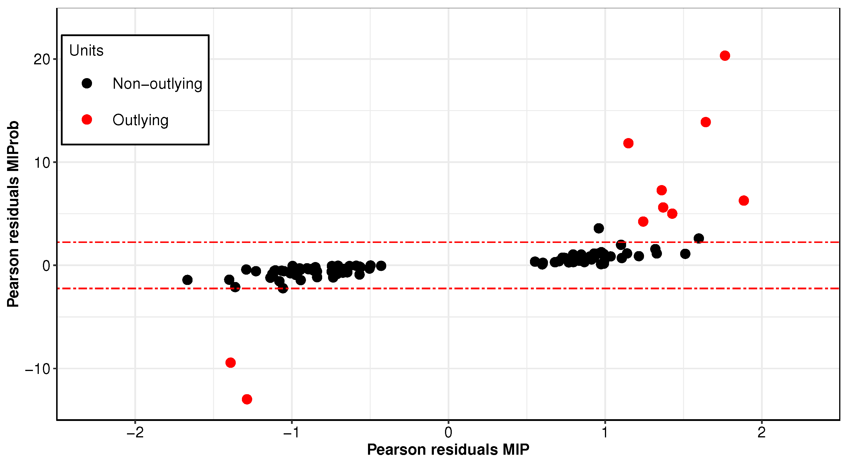
Figure 3 compares Pearson residuals for MIProb and MIP estimators. The outlying cases detected by MIProb, which are highlighted in red, deviate substantially from the remaining observations and are undetected by the non-robust MIP algorithm. Moreover, focusing on the set of features selected by MIProb, Figure 4 compares the boxplots of outliers selected by MIProb against the remaining non-outlying cases. We notice that the two distributions are indeed quite different for variables such as “bee2”, “gdd”, “EW” and “ITL”. This provides further evidence that the data set contains some outlying cases which significantly differ from the rest of the points.

6. Discussion

We propose a discrete approach based on $L_0$-constraints to simultaneously perform feature selection and multiple outlier detection for logistic regression models. This is important since modern (binary) classification studies often encompass a large number of features, which tends to increase the probability of data contamination. Outliers need to be detected and treated appropriately, since they can hinder classical estimation methods. Specifically, we focus on the logistic slippage model, which leads to the exclusion (or trimming) of the most influential cases from the fit, and a “strong” sparsity assumption on the coefficients. To solve such a double combinatorial problem, we rely on state-of-the-art solvers for mixed-integer conic programming which, unlike existing heuristic methods for robust and sparse logistic regression, provide guarantees of optimality even if the algorithm is stopped before convergence. Our proposal, MIProb, provides robust and sparse estimates with an optional ridge-like penalization term.

MIProb, outperforms existing methods in our simulation study. It provides sparser solutions with lower false positive and negative rates for both feature selection and outlier detection while maintaining stronger predictive power under most settings. Moreover, MIProb performs very well in our honey bee overwintering survival application. Based on three years of publicly available data from Pennsylvania beekeepers, it outperforms existing heuristic methods in terms of predictive power, robustness and sparsity of the estimates, and it produces results consistent with previous studies [18]. In particular, we found that weather variables appear to be strong contributors. Winter total precipitation and growing degree days are positively associated with honey bee survival, while the mean temperature of the driest quarter and the precipitation of the warmest quarter show a negative association. Moreover, our results indicate that the lower the exposure to pesticide (i.e., as their distance increases) the higher honey bee survival is. These findings are important in order to understand the main drivers of honey bee loss and highlight the importance of multi-source data to study and predict honey bee overwintering survival.

Our work can be extended in several directions. We are exploring additional and more complex simulation settings (e.g., higher dimensionality, collinear features, etc.). We did not experiment with the ridge-like penalty in the current paper, but this is an important tool and requires further investigation. However, computing time is currently the main bottleneck to more extensive exploration. Thus, in the future, we plan to consider additional modeling strategies that can reduce the computational burden. For instance, developing more suitable big-$\mathcal{M}$ bounds and using outer approximation techniques with dynamic constraint generation and first-order techniques as in [30]. We are also exploring more efficient tuning strategies for the sparsity and trimming levels, as well as the ridge-like parameter, if present. Utilizing approaches such as warm-starts or integrated cross-validation [56] can substantially reduce the computational burden for subsequent runs of the MIP algorithm, and allow better tuning. If the trimming level for MIProb is inflated, a re-weighting approach may also be included in order to increase the efficiency of the estimator as in [10], as well as approaches based on the forward search [45]. However, larger trimming levels might increase the computational burden, and the procedure does not take into account the feature selection process. Thus, the forward search might be combined with diagnostic methods that simultaneously study the effect of outliers and features [78]. Moreover, the theoretical properties of our procedure require further investigation, and its extension to other generalized linear models such as Poisson or multinomial regressions is of great interest.

Source code for the implementation of our procedure and to replicate our simulation and application results is openly available at https://github.com/LucaIns/SFSOD_logreg (accessed on 29 July 2021).