Abstract
We predict the finite population proportion of a small area when individual-level data are available from a survey and more extensive household-level (not individual-level) data (covariates but not responses) are available from a census. The census and the survey consist of the same strata and primary sampling units (PSU, or wards) that are matched, but the households are not matched. There are some common covariates at the household level in the survey and the census and these covariates are used to link the households within wards. There are also covariates at the ward level, and the wards are the same in the survey and the census. Using a two-stage procedure, we study the multinomial counts in the sampled households within the wards and a projection method to infer about the non-sampled wards. This is accommodated by a multinomial-Dirichlet–Dirichlet model, a three-stage hierarchical Bayesian model for multinomial counts, as it is necessary to account for heterogeneity among the households. The key theoretical contribution of this paper is to develop a computational algorithm to sample the joint posterior density of the multinomial-Dirichlet–Dirichlet model. Specifically, we obtain samples from the distributions of the proportions for each multinomial cell. The second key contribution is to use two projection procedures (parametric based on the nested error regression model and non-parametric based on iterative re-weighted least squares), on these proportions to link the survey to the census, thereby providing a copy of the census counts. We compare the multinomial-Dirichlet–Dirichlet (heterogeneous) model and the multinomial-Dirichlet (homogeneous) model without household effects via these two projection methods. An example of the second Nepal Living Standards Survey is presented.
1. Introduction
In a study on health, one might need to know how many people are in excellent health, good heath, fair health, or poor health in different households within different counties in a state. The second Nepal Living Standards Survey has sparse counts of household members within wards (a district consists of wards) for four health status groups. We want to predict the finite population proportion of people in each health category in each ward based on a sample from the households within wards. Undoubtedly there is heterogeneity within wards, the small areas (e.g., Rao and Molina [1]), and not taking this into consideration when inference is made about the finite population proportions within each ward, could lead to biased estimates and to incorrect variability. We note that the work in this paper is an updated version of Nandram [2].
The World Bank has developed a method to link a sample survey to a Census using a clustered bootstrap method for poverty estimation (i.e., continuous income data). This method is biased for several reasons. One problem is the method that is used by the World Bank is Empirical Bayes that typically underestimates variance and can also be biased. Of course, the survey and the Census are never done at the same time, and this creates an additional bias. Recently Corral et al. [3] have improved this method considerably by incorporating survey weights and heteroscedasticity. Our method is different from theirs because it uses count data, not continuous income data, and it is fully Bayesian, not Empirical Bayes. Another major difference is that our method is computationally intensive.
In the Nepal Living Standards Survey (NLSS II or simply NLSS), an area is a ward and a sub-area is a household, which is a group of people ‘sharing the same pot’. Nepal is divided into strata, each stratum is divided up into districts, each district is divided up into wards (small areas), and each ward consists of households (sub-areas). Of course, one can model all these levels (a difficult task), but here we study wards and households for the largest stratum. The sampling design of the NLSS II used two-stage stratified sampling. A sample of psu’s was selected using PPS sampling and then 12 households were systematically selected from each ward. Thus, households have equal probability of selection. However, while individuals in a household has equal probability of selection, these probabilities will vary with the size of the households, and there are other adjustments (e.g., non-response). That is, over the entire Nepal, each individual has unequal probability of selection.
Five relevant covariates, which can influence health status from the same NLSS, are age, nativity, sex, area, and religion. Nandram et al. [4] created binary variables nativity (Indigenous = 1, Non-indigenous = 0), religion (Hindu = 1, Non-Hindu = 0), sex (Male = 1, Female = 0), and area (Urban = 1, Rural = 0). Older age and child age are more vulnerable than younger age. Indigenous people can have different health status from migrated people. Similarly, health status of urban and rural citizens could be different. Because these are individual features, they are not available in the census.
Nandram et al. [5] or Nandram et al. [4], henceforth NCFM, analyzed data from the health part of the questionnaire for the largest stratum that consists of a large number of households for binary data (good versus poor health). NCFM is an update of Nandram et al. [4] and we will refer to either one at various places. NCFM used a logistic regression model which has one random effect for each household, thereby helping to correct for over-shrinkage so common in small area estimation. Because there are numerous households, the computational time on the joint posterior density using standard Markov chain Monte Carlo (MCMC) methods is prohibitive. Therefore, the joint posterior density of the hyper-parameters is approximated using an integrated nested normal approximation (INNA) via the multiplication rule. The INNA method has an important advantage over the integrated nested Laplace approximation (INLA) because it is not needed to compute a very large number of modes. This approach provides a sampling based method that permits fast computation, thereby avoiding very time-consuming MCMC methods. Then, the random effects are obtained from the exact conditional posterior density using parallel computing. The unknown non-sample features and household sizes are obtained using a nested Bayesian bootstrap that can be done using parallel computing as well. For relatively small data sets (e.g., 5000 households), NCFM compared their method with the ‘exact’ MCMC method to show that their approach is reasonable. The approach in these data integration paper, denoted by DIP, is different in the following ways.
- NCFM analyzed binary health data; DIP analyzes polychotomous health data;
- NCFM used logistic; DIP uses a multinomial-Dirichlet–Dirichlet model for the sample counts;
- NCFM does not link the survey to the census; DIP does this;
- NCFM obtained the non-sample covariates and household sizes using the a Bayesian bootstrap; DIP uses information from the census through a record linkage;
- NCFM had to develop an approximate method, INNA, for model fitting; DIP makes no analytical approximation (only those based on MCMC);
- NCFM used the health covariates from the questionnaire; DIP does not use these health covariates because they are not available in the census;
- Finally, NCFM is a two-stage procedure; DIP is a one-stage procedure.
Therefore, DIP is an advance over NCFM and DIP goes in a different direction.
In this project, we have NLSS data in individual level and census data in household level. So one way to proceed is to ignore the covariates in the NLSS in order to proceed to inference about the finite population proportions, where we can use the covariates. We describe how to use these covariates in the concluding remarks. A further problem is that while the wards in the NLSS match the wards in the Census, the households do not (i.e., there are no labels to make this matching). So we have to match the households in the Census and the NLSS using a record-linkage procedure. There are six variables at the household level (including household sizes) and three variables at the ward level; these latter variables cannot be used for matching but they can be used for prediction. Most of the variables are either discrete or just proportions.
We chose nine relevant covariates, generally used for analysis, that can influence welfare status, and per capita consumption for modeling; see Nepal Living Standards Survey [6]. They are (i) household size, (ii) proportion of kids aged 0–6 in the household, (iii) proportion of kids aged 7–14 in the household, (iv) abroad migrant, (v) house temporary, (vi) house owned, (vii) proportion of households with cooking fuel LP/gas in ward, (viii) proportion of households with land-owning females in municipality/ VDC, and (ix) proportion of kids 6–16 attending school in municipality/VDC (VDC stands for village development community). Note that six of these covariates (i–vi) are available at the household level and the other three (vii–ix) are ward level covariates. These covariates are available in both the NLSS and the 2001 census. We use all these covariates in our modeling, but we use only the first six for linking NLSS with the census. It is worth noting that not all the covariates used for linking the NLSS and the census are discrete.
We matched the Census and the NLSS as follows. We started by matching all six covariates, and this procedure provides a majority of the matches. For those that did not match, we went down to five variables at a time (five sets of matching), then four variables, and so on. At the end there were some variables that did not match. For these we used a nearest neighbor matching procedure via a distance function. Then, the final dataset consists of households within wards, sampled and non-sampled. The sampled households have responses (counts in different health status). There are also wards not sampled. There are 101 sampled wards and 12,133 non-sampled wards (One ward did not have the 12 sampled households; to maintain a balance, we eliminated it from further consideration). Prediction is needed for the sampled households in the sampled wards and the households of the 101 sampled wards and all the households of the 12,133 non-sampled wards.
Our complete procedure is the following. First, we describe the two models, multinomial-Dirichlet (area-level, homogeneous) model and the multinomial-Dirichlet–Dirichlet (sub-area, heterogeneous) model. We fit both the homogeneous and heterogeneous models using a Markov chain Monte Carlo sampler. For the small-area model, we use the Gibbs sampler and for the sub-area model we use the Metropolis–Hastings sampler. Nandram et al. [4] made approximation to do the posterior density and showed empirically that the approximation is reasonable. However, we use this approximation to construct a proposal density in the sub-area model. From these models, we generate the super-population proportions that are then linked to the census data through the covariates. Noting that the proportions are the same for each household in a ward, we generated independent and identical proportions for the households within a ward. Then, we fit regression models to the logarithm of the proportions (iterates) to get the regression coefficients. We have used either iterative re-weighted least squares (IRLS) or the nested error regression (NER) model to get the regression coefficients that are then used to generate the counts for both the sampled and non-sampled households in both the sampled wards and the non-sampled wards. The rest is standard Monte Carlo procedures to infer a posteriori the finite population proportions for the wards.
The paper has five more sections. In Section 2, we review the two-stage multinomial-Dirichlet model (homogeneous) and we present the multinomial-Dirichlet–Dirichlet model (heterogeneous). In Section 3, we show how to fit the two models. Specifically, first we review how to fit the multinomial-Dirichlet model and then we give more detail about the multinomial-Dirichlet–Dirichlet model. In Section 4, we describe how to make inference about the finite population proportions. Specifically, we show how to connect the NLSS to the Census. In Section 5, we show how to analyze Nepal’s data. We also describe how to calibrate the survey weights to the Census, a procedure that is potentially useful for linking a survey and a census. Section 6 has concluding remarks and there are discussions on how to improve the current method. A technical detail is given in the Appendix A.
2. Hierarchical Bayesian Models
We describe the two models we study in this section. In Section 2.1, we review the multinomial-Dirichlet model and in Section 2.2 we describe the multinomial-Dirichlet–Dirichlet model, an extension of the multinomial-Dirichlet model. It is necessary to include both household effects and ward effects in a model; the multinomial-Dirichlet model can handle one effect (household or ward). The multinomial-Dirichlet–Dirichlet model is a sub-area model, the wards are the areas and the households are the sub-areas, and, therefore, it can be called a sub-area model. The sub-area models are a special class of models used in small area estimation and they actually fall under the general class of two-fold models (e.g., Nandram [7], Lee et al. [8], and the references therein).
Let the cell counts for the ℓ contingency tables of c cells be That is, there are ℓ one-way contingency tables each with households having , where c is the number of health groups (i.e., c cells with individuals). There are sub-areas (households) within the area (ward) in the population and of these sub-areas are sampled. There are L areas in the population and ℓ of them are sampled. Here, we take . We use the dot notation (e.g., ).
2.1. Multinomial-Dirichlet Model
We first consider a homogeneous area (ward) level model and we will write down the model for the sample (the model is assumed to hold for the whole population). We assume
Here are sufficient statistics and under this assumption, the hierarchical Bayesian model is
where, without any prior information, we have taken and to be independent; see Nandram [9] for computations and Nandram and Sedransk [10] for an interpretation of . The prior, , is proper and convenient, and we have been using it for many years.
We will call this model the homogeneous model or the area-level model. This model incorporates only the multinomial counts in the ℓ areas, and it does not take account of the sub-areas, hence the name homogeneous or area-level model. When inference about the sub-area is of interest, one can use the area-level model with the conditional posterior density, (i.e., draws of can be made from it), but this is not optimal because it does not include the household effects.
2.2. Multinomial-Dirichlet–Dirichlet Model
Here, we write down the model for the sample , but the model is assumed to hold for the entire population of areas and sub-areas, .
Therefore, letting , for the sample the multinomial-Dirichlet–Dirichlet model assumes that
where, without any prior information, we have taken , , and to be independent. For simplicity, we have used a single (i.e., not depending on area). It is important to note the dependence of the on j (i.e., both ward and household effects). When is large, the household effects will disappear.
Inference about the and the under the homogeneous model can be obtained by using samples from their joint posterior densities. This is an intermediate step to make inference about the finite population proportions.
Because the counts in the households are sparse for many households (see discussion later), it is necessary to adjust the heterogeneous model. The counts in the last cell are mostly zeros, so we decided to combine the last two cells. Even as such it is still sparse. However, we noticed an order restriction of the proportions of household members in the three cells. So we impose the order restriction . The order restriction also helps to provide a better MCMC algorithm. The order restriction is not applied to the homogeneous model.
3. Bayesian Computations
In Section 3.1, we present a brief discussion of the computations for the multinomial-Dirichlet model; see Nandram [9] for a more sophisticated method based on the Metropolis–Hastings sampler. In Section 3.2, we give a more detailed description of the computations for the multinomial-Dirichlet–Dirichlet model; this uses the Metropolis–Hastings sampler. Specifically, we show how to overcome a computational difficulty by numerical integration.
3.1. Multinomial-Dirichlet Model
The conditional posterior density of . Thus, one can obtain Rao-Blackwellized density estimators of having obtained a sample of from their joint posterior density.
It is easy to show that
where we have transformed to , and any of the arguments must be set to unity if or , very likely for some cells. So that this posterior density is well defined for all , .
It is easy to use the griddy Gibbs sampler, not the Metropolis–Hastings sampler (Nandram [9]), to draw samples from . Each of the conditional posterior densities is drawn using a grid method. This mixes very well and it converges to the target distribution very quickly.
3.2. Multinomial-Dirichlet–Dirichlet Model
It is straightforward to see that
Again, Rao-Blackwellized density estimators of can be easily obtained. It is useful to note that this conditional posterior density depends only on and , but not on the other parameters. Then, integrating out the , we get the joint posterior density of ,
where, is the Dirichlet function, and for convenience, we use
Note that the conditional posterior density of given is the product of two parts. The first part is , which is complicated, and the second part is , the Dirichlet prior distribution. We can think of the posterior density as the product of two densities, one proportional to , and the other one is . In fact, we can think of , as the posterior density for each area as in Nandram [9]. That is, this is just the posterior density that Nandram [9] used to obtain a Metropolis–Hastings sampler to draw samples from; see Appendix A of Nandram et al. [4].
Note that and are not directly connected to the counts even after integrating out the . This indicates that there will be difficulties in running a Markov chain Monte Carlo sampler. Therefore, further integration is necessary; we also need to integrate out the (i.e., need to draw the parameters simultaneously), but this is not possible analytically. We will describe a numerical method to to integrate out the . Nandram [4] has an analytical approximation that we have emphasized therein. Our method to integrate out the is to use a representation of the Dirichlet distribution that is a product of beta distributions; see Darroch and Ratcliff [11] and Connor and Mossimann [12].
Let be a vector with c components such that . Assume that , where is a vector with c known elements. Then,
Let , . Then, .
Using this characterization on with , we get
Here, transforms to , where
The integration is easy to carry out by discretization over the range of the independent beta random variables, and , and we use the middle Riemann sum for integration.
We can now draw using a Metropolis sampler. The candidate generating density is the analytic approximation discussed in Nandram et al. [4]. We draw a sample of 10,000 iterates using the Gibbs sampler (to allow a “burn in” and thinning to get 1000 samples). We showed how to construct a proposal density for to run the Metropolis sampler (Nandram et al. [4]). We used a grid method to draw in this preliminary sample. Thus, we have samples from the approximate posterior density of . We transform these to where , , . Then, we fit a multivariate normal density to , where and are the mean and covariance matrix of the samples, and to complete the -variate Student’s t density on degrees of freedom, where is a tuning constant. We restart the algorithm if it is necessary.
The order restriction on (see below) is enforced by rejection sampling. Let us consider how this order restriction changes the conditional posterior densities (CPD’s) of and ; notice . Thus, the order restriction is really
and this is a key inequality. Now, we need the support of the cpd of given the other parameters and the support of the cpd of given other parameters. In Appendix B of Nandram et al. [4] (2018), we showed that that given , the support of is and given , the support of is We have drawn samples from the cpds of and using the grid method.
Both the Metropolis sampler for the exact computations and the Gibbs sampler show good performance as evident by the trace plots, auto-correlations, Geweke test of stationarity, the effective sample sizes and the jumping rate of the Metropolis sampler.
To draw the , we use a Metropolis algorithm with the approximate Dirichlet distribution (Nandram [9]) as the proposal density to draw samples of independently given and data. We ran each Metropolis sampler 100 times (500 times did not make a significant difference) and picked the last one. If the Metropolis step fails (jumping rate is not in (0.25, 0.75)), we use the griddy Gibbs sampler within this Metropolis step. Parallel computing can also be used in this latter step. This is performed in the same manner for the exact method (i.e., numerical integration). For our application with 101 wards, this latter step runs very fast. Of course, with a much larger number of wards, the computing time will be substantial, but now parallel (embarrassingly) computing is available.
4. Inference for Finite Population Proportions
We have now obtained samples , say . The next step is to link these to the census. The census has covariates , a vector of () components, including an intercept, for all households, sampled or non-sampled. There are three parts, the sampled households in the sampled wards, the non-sampled households in the sampled wards and the non-sampled households in the non-sampled wards.
We use the following steps to implement the projection procedure.
- Model the for each (independent regression-type analyzes)see Agresti [13] for the multinomial logit transformation;
- Project for each k using the model (entire census);
- Define new using the ,and , ;
- Draw the from multinomial models; obtain copies of the census counts.
This regression analysis will be performed for each of the M samples of . We can obtain all the non-sampled for all M iterates in the same manner. Having obtained the cell probabilities, the multinomial counts can be generated for each of the M iterates, thereby obtaining a large sample (size M) of contingency tables for the entire census. We have two methods of doing this operation in a comprehensive manner.
4.1. Iterative Re-Weighted Least Squares Method
We have used the ensemble M-estimation model in small area estimation; see Chambers and Tzavidis [14], where the regression coefficients are estimated using iterative re-weighted least squares (IRLS). This is an attractive non-parametric procedure for small area estimation because there are no random effects to model, but random effects come out as summaries of q-scores. A good review paper is given by Dawber and Chambers [15]. This is directly related to the procedure mentioned above.
Let denote the responses and the covariates for unit j in area i, . We string out these values and relabeling, the responses are and the covariates are for . In the IRLS, for each q in is obtained by solving
where are the median absolute deviation of and the weights are
with . Here, I is the indicator function, is a tuning constant and the second term is the Huber influence function. In our analysis, we have set . In the ensemble M-estimation model, the IRLS procedure is executed for every q on a fine grid in . Then, the q-score solves the equation,
The random effects are then obtained as a summary (e.g., median) of the for area i, denoted by . Now, are the estimated regression coefficients for this area.
The IRLS is performed sequentially as follows. Start up the process using standard least square estimators, obtain the residuals and the median absolute deviation of the residuals, and finally the weights. Then, use the weights and the median absolute deviation to get the first re-weighted least square estimates of the regression coefficients. Now iterate the process for each value of q in a fine grid in ; we have used (0.10, 0.90) because of computational instability.
4.2. Nested Error Regression Method
The second method is the nested error regression (NER) model; see Battese et al. [16]. We use the full Bayesian version of the NER model which was originally developed by Toto and Nandram [17] and later applied to poverty estimation by Molina et al. [18].
Letting, for each k, , the Bayesian NER model is
Again, the Bayesian NER model is applied times for each of the M samples.
The joint posterior density is proper provided the design matrix is full rank. Molina et al. [18] need an additional condition for posterior propriety, and it turns out that this condition is not necessary; see Appendix A. However, we note here that the NER model is not robust against outliers and non-normality (e.g., see Chakraborty et al. [19], and Gershunskaya an Lahiri [20]. There is a clear advantage to use M-estimation, albeit it is more complicated and computationally intensive.
The posterior density of can be obtained apart from the normalization constant, and all the other conditional posterior densities, in order to use the multiplication rule to get the joint posterior density, are in standard forms. Therefore, it is easy to get a sample from the joint posterior density using the composition method (i.e., the multiplication rule of probability). Draws from the posterior density of is obtained using a fine grid on ; see Appendix A. This method is very fast, and much faster than the IRLS, because it simply uses random draws, not a Markov chain, and the IRLS has to be done on a fine grid. Although the IRLS projection method took more than 10 h even with a parallel system with 32 processors, the NER method took about 5 h on a single processor.
Of course, the ensemble M-quantile estimation model is non-parametric, but there may be some difficulties in finding the q-scores near 0 and 1, if these are actually needed.
4.3. Bayesian Projective Inference
We can perform either a Bayesian predictive inference or a Bayesian projective inference about the finite population proportions for each ward or even at a more micro level for each household. Predictive inference means that the non-sampled households are filled in while projective inference means that all households (sampled and non-sampled) are filled in. We have actually used the projective method for the NLSS sampled households and the Census because smoothed estimates of the household proportions may be needed for the sampled households.
For the non-sampled households in non-sampled wards (areas), we use the IRLS estimates at ; see Dawber and Chambers [15]. For non-sampled households in a sampled ward, we use an average of the quantiles corresponding to the sampled households; see Dawber and Chambers [15]. For the NER model, we would need to use for the non-sampled households within sampled wards via the posterior samples of the (already drawn). For the non-sampled wards, we will need to use a draw from the the prior distribution of (no-data posterior density) and compute .
Finally, in a projective method, we will obtain all the for both the samples and the non-samples. Then, we will draw the cell counts for all households. For each ward, sum all the cell counts of the households in a ward, and divide by the population size (known) to get the finite population proportions in the three cells.
5. Analysis of Nepal’s Data
We use data from the Nepal Living Standards Survey (NLSS II, Central Bureau of Statistics, [6]) to illustrate our methods. In Section 5.1, we describe the 2001 Census and NLSS II. In Section 5.2, we apply our method to Terai Rural stratum, the narrow strip of rural areas in southern side of Nepal bordering India; see Figure 1 that shows the districts, not the lower levels of wards and households. We note that in the Terai Rural stratum the wards are scattered in the whole strip (In this region, there are 29 Metropolitan areas, each with at least 9 wards, roughly 300 wards in total, and these Metropolitan areas are obviously not included in the Terai Rural stratum).
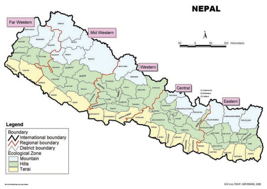
Figure 1.
Map of Nepal showing the Terai Region.
5.1. Census and NLSS II
The Census and NLSS II (simply NLSS) are the same as described in Nandram et al. [4]. So we do not repeat the discussion here in detail, but below we give the key points.
NLSS is a national household survey in Nepal, actually population based (i.e., interviews are done for individual household members). NLSS follows the World Bank’s Living Standards Measurement Survey methodology with a two-stage stratified sampling scheme, which has been successfully applied in many parts of the world. It is an integrated survey which covers samples from the whole country and runs throughout the year. The main objective of the NLSS is to collect data from Nepalese households and provide information to monitor progress in national living standards. The NLSS gathers information on a variety of subjects. It has collected data on demographics, housing, education, health, fertility, employment, income, agricultural activity, consumption, and various other subjects. We choose the polychotomous variable, health status, from the health section of the questionnaire.
Health status is covered in Section 8 of the questionnaire, which collected information on chronic and acute illnesses, uses medical facilities, expenditures on them and health status. The health status questionnaire is asked about every individual that was covered in the survey, and the questionnaire has four options (excellent, good, fair, poor), but because the fourth cell is overly sparse, we combine fair and poor into a single cell (renamed poor).
In the NLSS, Nepal is divided into wards/sub-areas (psu’s) and within each ward/sub-ward there are a number of households. The sample design of the NLSS used two-stage stratified sampling. A sample of psu’s was selected using PPS sampling and then 12 households were systematically selected from each ward. Thus, households have equal probability of selection. However, while individuals in a household have equal probability of selection, the survey weights have various adjustments, so they vary with the size of the households and the individuals. For this project we will ignore the survey weights because this needs a multinomial logit model that we are currently studying. However, we have discussed alternatives in the concluding remarks.
Nandram et al. [5] chose nine relevant covariates which can possibly influence health and they are available in the 2001 census data. Six of the covariates are at the household level and three at ward level. At the ward level the NLSS and the Census are matched, but the households are not matched. Therefore, only the household variables are used for matching, but all covariates are used for projection.
There are six strata and we study the Terai Rural stratum, the largest stratum in Nepal. It has 102 wards/sub-wards with 1224 households in the sample of 12,239 wards in the population (sample frame) with 1,686,317 households with 9,744,810 people. The number of people in the sample is 6979 with 3901 in the first cell, 2921 in the second cell, and 157 in the third cell with percentages 55.9%, 41.9%, and 2.2%. The sample of 6979 will speak for 9,744,810 people (i.e., a sample of just 0.07%). So we have imposed an order restriction over the three cells to assist the computations; specifically, we have taken .
5.2. Comparisons
We compare the two models (Hom, Het) and the two projection methods (IRLS, NER). The NER model is not robust against outliers and non-normality, but M-estimation, based on the IRLS, is robust. Here, we compare the four scenarios: (IRLS,Het), (IRLS, Hom), (NER, Het), and (NER, Hom).
In Table 1, we see that the non-sampled part of the population dominates the inference. As summaries, we use posterior means (PM) and posterior standard deviation. There is a small, but important, selection bias. Considering the proportion of people in excellent health, the PMs for the four scenarios (IRLS, Het), (IRLS, Hom), (NER, Het), and (NER, Hom) are, respectively, , , , for the sample and , , , significantly larger for the non-sample. This selection bias can be mitigated when the survey weights are incorporated into the model. Survey weights have various adjustments (e.g., non-response)

Table 1.
Comparison of IRLS and the NER projective methods, the sub-area (Het) and the area-level (Hom) models with respect to posterior inference about the finite population proportions by health classes (three proportions).
Inference for the non-sampled part of the population is virtually the same as the whole population. (Compare (b) and (c) of Table 1). This is not surprising because there are 101 wards in the sample and 12,133 wards in the non-sample (i.e., the sampling fraction, , is very small).
In Figure 2, Figure 3, Figure 4, Figure 5, Figure 6 and Figure 7, we further compare the four groups. Each of these plots contains 36,702 points corresponding to the three health classes and 12,234 wards and the plots are for the two posterior means of the finite population mean. It is not the intention of these scatterplots to select a model; this is a difficult task in the current application because we need to assess a two-stage procedure. Rather our intention is to show similarities in the posterior means over the four scenarios.
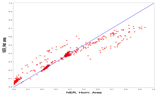
Figure 2.
Comparison of the homogeneous model and the heterogeneous model under the NER method for prediction of the finite population proportions (posterior means) for all wards.
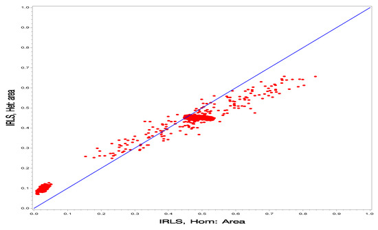
Figure 3.
Comparison of the homogeneous model and the heterogeneous model for prediction of the finite population proportions (posterior means) for all wards under the IRLS method.
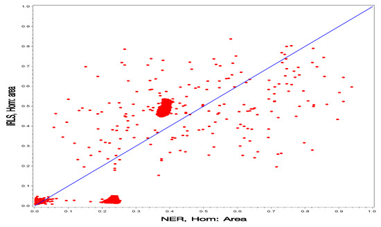
Figure 4.
Comparison of the NER and IRLS projection methods under the homogeneous model prediction of the finite population proportions (posterior means) for all wards.
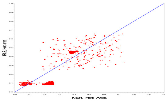
Figure 5.
Comparison of the NER and IRLS projection methods under the heterogeneous model for prediction of the finite population proportions (posterior means) for all wards.
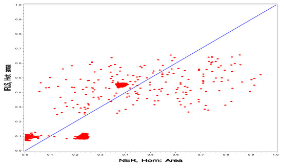
Figure 6.
Comparison of the homogeneous model under the NER projection method and the heterogeneous model under the IRLS method for prediction of the finite population proportions (posterior means) for all wards.
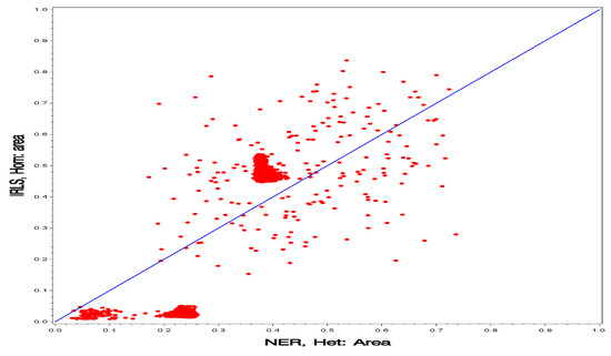
Figure 7.
Comparison of the heterogeneous model under the NER projection method and the homogeneous model under the IRLS method for prediction of the finite population proportions (posterior means) for all wards.
In Figure 2 and Figure 3, we compare the two models (Hom vs. Het). In Figure 2, we can see clearly the difference between the two models for the NER projection method. The points are scattered around the 45-degree straight line with smaller slope. In Figure 3, we can see clearly the difference between the two models for the IRLS projection method. The points are scattered around the 45-degree straight line with smaller slope, but much more concentrated than the NER projection method.
In Figure 4 and Figure 5, we compare the two projection methods (IRLS vs. NER). In Figure 4, we can see clearly the difference between the two models for the NER projection method. The points are scattered around the 45-degree straight line with smaller slope, but much more spread out. In Figure 5, we can see clearly the difference between the two models for the IRLS projection method. The points appear to be in a rectangle with the 45-degree roughly along its diagonal.
In Figure 6 and Figure 7, we look at the interaction of the two factors (model, projection methods). Again, the clouds of points cross the 45-degree straight line in both plots and there is large spread.
As a summary, Figure 2 shows that the PMs for (NER, Het) are similar to those of (NER, Hom) and Figure 3 shows that the PMs for (IRLS, Het) are similar (IRLS, Hom). Figure 4, Figure 5, Figure 6 and Figure 7 show wide disparities among those scenarios. These figures are intended to show similarities among the PMs for two scenarios.
As suggested by a reviewer, we have also studied the finite population mean for each of the 101 wards, each of the 3 cells and each of the 4 scenarios at a more detailed level. We have studied PM, PSD, coefficient of variation (CV) and 95% highest posterior density interval (HPDI), and we make comparison with the observed sample proportion, , of people in each cell. The third cell is empty for many wards so that for these cells (Of course, this is not a sensible estimate and it will be shrunk away from under all scenarios). As we have a table with rows, we have selected three wards for further study; see Table 2, Table 3 and Table 4.
Table 2.
Example 1: Comparison of the four scenarios (IRLS, Het), (IRS, Hom), (NER, Het), (Ner, Hom) with respect to posterior inference about the finitas population proportions by health classes (three proportions).
Table 3.
Example 2: Comparison of the four scenarios (IRLS, Het), (IRS, Hom), (NER, Het), (Ner, Hom) with respect to posterior inference about the finite population proportions by health classes (three proportions).
Table 4.
Example 3: Comparison of the four scenarios (IRLS, Het), (IRS, Hom), (NER, Het), (Ner, Hom) with respect to posterior inference about the finite population proportions by health classes (three proportions).
First, we consider Table 2. We see that the CVs are all acceptable. The PSDs for Het is always larger than that for Hom, but they are acceptable as the CVs are reliable measure. We notice that for cells 1 and 2, all s lie in the corresponding 95% HPDIs. This is comforting. However, for cell 3 (sparse cell), for (IRS,HOM) and (NER,HOM), is to the right of the 95% HPDIs. This is to be expected because it is difficult to estimate the finite population proportion corresponding to the third sparse cell. In general, PSDs are smaller under Hom than Het.
Second, we consider Table 3. The results are generally similar to Table 2. For the third cell is to the left of the 95% HPDI for (IRLS,HET) and to the right for (IRLS,HOM).
Third, we consider Table 4 that has zero counts in the last cell over all households. In this case the PMs and PSDs are different over the four scenarios. Again the PSDs are smaller under Hom. With zero counts in the third cell, all the 95% HPDI do not contain . This is not comforting but it does show the over-shrinkage that this can cause; yet these estimates can be reasonable.
It is not possible to judge which scenario is better based on NLSS data only. The IRLS has no distributional assumption and it is robust against outliers. The Het has an extra layer (more parameters) and, therefore, it can mislead someone with with a bit larger variability. NER has normality assumptions that may be incorrect and it is well known that it is not robust to outliers. Its small variation can be misleading. If one needs a simple model, I believe that the (NER,Hom) should be used. However, we should not rule out the (IRLS,Het) because it is versatile. There are difficulties with the empty third cell anyway. It is possible to know which is the right scenario by doing a large simulation study, but this is outside the scope of the current paper. Standard diagnostics do not apply because we are using a two-stage procedure.
5.3. Calibration
It is necessary to calibrate the NLSS to the Census using survey weights and census covariates. We would need to do this for each sampled ward. There are non-sampled households in each ward. We have all the household covariates for all the sampled wards in the Census. So we have the totals for all the households within a ward. We do not know the household sizes for the sampled wards; we have used data fusion to fill these in by using the household sizes of the sample to donate to the non-sampled household within a ward. Although we have not done this yet, we note that this will be a useful addition to our procedure.
Let , denote the covariates, including an intercept, in the sample survey and denote the survey weights. Let , where N is the number of households in the census. The method is described for households but it can be used for individuals. Then, . The survey weights are calibrated when we can find such that , where are the survey weights; a distance function is used to measure closeness between the and the . Haziza and Beaumont [21] gave a very informative and clear pedagogical review of this method.
Let the original survey weights in the NLSS be . We search for a calibrated weighting system , such that , the calibration equation. We want to the , to be as close as possible to . Haziza and Beaumont [21] judge closeness by a distance function, , where
- and ;
- is differentiable, , and strictly convex.
One needs to minimize over , where denote the importance of unit j, subject to the constraint . We present some details here on how to solve the Lagrangian system of equations for a general . (we have made some changes to Haziza and Beaumont [21]).
We give the final step on how to numerically compute for a general . Consider the function,
where are Lagrangian multipliers.
Differentiating with respect to , we get
Therefore,
Here, our method differs from Haziza and Beaumont (2020) who used the Newton–Ralphson method. We use the Nelder–Mead algorithm to minimize
over , forcing each component down to zero, to get . The weights are then,
In our case, we use the simple Euclidean distance. This gives close form answers; apparently this was not recognized by Haziza and Beaumont (2017). We choose . For , is a legitimate distance function because , , , and so is strictly convex. Additionally, . In this case, we have
That is,
and
Therefore, assuming A is invertible, and the calibrated weights are .
6. Concluding Remarks
We have shown how to obtain copies of the contingency tables of the 12,234 wards in the Nepal Census. We have actually studied the largest stratum among six strata of Nepal, Terrai Rural. Our procedure can be applied to each of the six strata in much the same way. No new methodology is needed. However, this matching procedure has been a very extensive endeavor. One might ask about a spatial analysis. One would like to incorporate a spatial effect among the households; unfortunately, there are no lists with the neighborhood of each household, but there is a list of the neighborhoods of the wards and the districts. Incorporating spatial effects at the district or ward level is not beneficial (i.e., too coarse).
It is possible to incorporate survey weights into our homogeneous and heterogeneous models. Nandram et al. [4] described one method to incorporate survey weights. Here, we suggest a simpler method, where our procedure described in this paper can be used almost immediately. Let denote the standardized survey weights of the individual in the household in the ward, , . Potthoff et al. [22] showed how to obtain the standardized weights under the assumption that the individual responses are independent but not identically distributed (each individual has a different mean and variance); so we apply the standardization within ward but the responses of the household members might be correlated. This result can be generalized easily to a cluster (i.e., intra-class correlation). Let denote which cell the individual falls in the household within ward (i.e., if it falls in cell t and 0 for all other cells. Then, the adjusted cell counts are . Our procedure can simply be applied immediately to these adjusted cell counts.
There are five relevant covariates that are normally used to study health status from the same NLSS survey. They are age, nativity, sex, area, and religion, and they are mostly binary. These health covariates are studied in Nandram et al. [5]. Here, our procedure does not apply directly. However, the iterates can be obtained by fitting a multinomial logit model similar to the homogeneous and the heterogeneous models. However, this is not easy. Another way is to partition the age variable, say young and old (binary), thereby making six categorical variables to form cells and one can fit the heterogeneous model using the procedure in this paper. However, one danger is the sparseness of the table. However, one can certainly eliminate some cells that are structural zeros.
One of the problems we encountered is which model to use. This can be figured out by doing a simulation study. One can draw samples that have little to do with any scenario and fit all scenarios. Yet this is not so simple.
Another problem is how to obtain a model that takes care of district estimates, a kind of benchmarking. Because the districts are very large, it easy to obtain a reliable estimate for each district. One can, therefore, benchmark the ward estimates or household estimates to the districts to obtain a more robust model. It is also possible to do a sub-sub-area model.
Funding
This research received no external funding.
Informed Consent Statement
This is a statistical data analysis and no human subjects were used or identified.
Data Availability Statement
The data, used in this paper, are confidential, but public-used data can be purchased from the Central Bureau of Statistics, Nepal.
Acknowledgments
The author thanks Lu Chen and Binod Manandhar for providing the data, and for collaboration on earlier work. This research was supported by a grant from the Simons Foundation (#353953, Balgobin Nandram). The author thanks the two reviewers for their comments. Additionally, it was a privilege for me to present this paper at JSM2020 in an invited session, organized by Malay Ghosh, to celebrate Glen Meeden’s 80th birthday. Finally, Balgobin Nandram was also an invited speaker on this topic at the ISI2019 conference in Malaysia, a keynote speaker in Langenhop Lecture and Southern Illinois University at Carbondale Probability and Statistics Conference, 2018, and an invited speaker in the Department of Statistics at Kyungpook National University, Daegu, South Korea, 2018.
Conflicts of Interest
The authors declare no conflict of interest.
Appendix A
We state the conditional posterior densities from Molina et al. [17]. We find that the condition, , where is a small positive constant, is not necessary. This eliminates the sensitivity analysis on .
Defining ,
If the are survey weights, , the population size, and these must be normalized so that , the effective sample size; see Potthoff et al. [22]. However, note that these do not exist (not defined) for non-samples. Therefore, for prediction something like surrogate sampling (Nandram [23], Nandram and Choi [24]) has to be done (In our application here, the survey weights are assumed to be unity).
First,
Observe that the mean and variance of are defined for all values of in . When , is a point mass at 0 and when , .
Second, letting
where . Again, observe that the mean and variance of are defined for all values of in .
Third, letting
Again, observe that is defined for all values of in .
References
- Rao, J.N.K.; Molina, I. Small Area Estimation, 2nd ed.; Wiley: New York, NY, USA, 2015. [Google Scholar]
- Nandram, B. A Bayesian Method to Linking a Survey and a Census. In Proceedings of the American Statistical Association, Survey Research Methods Section, Virtual Conference 2020, Online, 2–6 August 2020; pp. 1669–1688. [Google Scholar]
- Corral, P.; Molina, I.; Nguyen, M. Pull Your Small Area Estimates up by the Bootstraps. In Policy Research Working Paper, World Bank Group, Poverty and Equity Global Practice; World Bank: Washington, DC, USA, 2020; pp. 1–52. [Google Scholar]
- Nandram, B.; Chen, L.; Manandhar, B. Bayesian Analysis of Multinomial Counts from Small Areas and Sub-areas. In Section on Bayesian Statistical Science; American Statistical Association: Alexandria, VA, USA, 2018; pp. 1140–1162. [Google Scholar]
- Nandram, B.; Chen, L.; Fu, S.; Manandhar, B. Bayesian Logistic Regression for Small Areas with Numerous Households. Stat. Appl. 2018, 16, 171–205. [Google Scholar]
- Central Bureau of Statistics. Nepal living Standards Survey Report. In Statistical Report Volume 1; Central Bureau of Statistics Thapathali: Kathmandu, Nepal, 2004. [Google Scholar]
- Nandram, B. Bayesian Predictive Inference of a Proportion Under a Two-Fold Small Area Model. J. Off. Stat. 2016, 32, 187–208. [Google Scholar] [CrossRef]
- Lee, D.N.; Nandram, B.; Kim, D. Bayesian Predictive Inference of a Proportion Under a Two-Fold Small Area Model with Heterogeneous Correlations. Surv. Methodol. 2017, 43, 69–92. [Google Scholar]
- Nandram, B. A Bayesian Analysis of the Three-stage Hierarchical Multinomial Model. J. Stat. Comput. Simul. 1998, 61, 97–126. [Google Scholar] [CrossRef]
- Nandram, B.; Sedransk, J. Bayesian Predictive Inference for a Finite Population Proportion: Two-stage Cluster Sampling. J. R. Stat. Soc. 1993, 55, 399–488. [Google Scholar] [CrossRef]
- Darroch, J.N.; Ratcliff, D. A Characterization of the Dirichlet Distribution. J. Am. Stat. Assoc. 1971, 66, 641–643. [Google Scholar] [CrossRef]
- Connor, R.J.; Mosimann, J.E. Concepts of Independence for Proportions with a Generalization of the Dirichlet Distribution. J. Am. Stat. Assoc. 1969, 64, 194–206. [Google Scholar] [CrossRef]
- Agresti, A. Categorical Data Analysis, 3rd ed.; Wiley: New York, NY, USA, 2012. [Google Scholar]
- Chambers, R.; Tzavidis, N. M-Qunatile Models for Small Area Estimation. Biometrika 2006, 93, 255–268. [Google Scholar] [CrossRef]
- Dawber, J.; Chambers, R. Modelling Group Heterogeneity for small Area Estimation Using M-quantiles. Int. Stat. Rev. 2019, 87, S50–S63. [Google Scholar] [CrossRef]
- Battese, G.E.; Harter, R.; Fuller, W.A. An Error-Components Model for Prediction of County Crop Areas Using Survey and Satellite Data. J. Am. Stat. Assoc. 1988, 83, 28–36. [Google Scholar] [CrossRef]
- Toto, M.C.S.; Nandram, B. A Bayesian Predictive Inference for Small Area Means Incorporating Covariates and Sampling Weights. J. Stat. Plan. Inference 2010, 140, 2963–2979. [Google Scholar] [CrossRef]
- Molina, I.; Nandram, B.; Rao, J.N.K. Small Area Estimation of General Parameters with Application to Poverty Estimators: A Hierarchical Bayesian Approach. Ann. Appl. Stat. 2014, 8, 852–885. [Google Scholar] [CrossRef]
- Chakraborty, A.; Datta, G.S.; Mandal, A. A Robust Hierarchical Bayes Small Area Estimation for Nested Error Linear Regression Model. Int. Stat. Rev. 2019, 87, S158–S176. [Google Scholar] [CrossRef]
- Gershunskaya, J.; Lahiri, P. Robust empirical best small area finite population mean estimation using a mixture model. Calcutta Stat. Assoc. Bull. 2018, 69, 183–204. [Google Scholar] [CrossRef]
- Haziza, D.; Beaumont, J.-F. Construction of Weights in Surveys: A Review. Stat. Sci. 2017, 32, 206–226. [Google Scholar] [CrossRef]
- Potthoff, R.F.; Woodbury, M.A.; Manton, K.G. “Equivalent Sample Size” and “Equivalent Degrees of Freedom” Refinements for Inference Using Survey Weights Under Superpopulation Models. J. Am. Stat. Assoc. 1992, 87, 383–396. [Google Scholar]
- Nandram, B. Bayesian Predictive Inference Under Informative Sampling Via Surrogate Samples. In Bayesian Statistics and Its Applications; Upadhyay, S.K., Singh, U., Dey, D.K., Eds.; Anamaya: New Delhi, India, 2007; pp. 356–374, Chapter 25. [Google Scholar]
- Nandram, B.; Choi, J.W. A Bayesian Analysis of Body Mass Index Data From Small Domains Under Nonignorable Nonresponse and Selection. J. Am. Stat. Assoc. 2010, 105, 120–135. [Google Scholar] [CrossRef]
Publisher’s Note: MDPI stays neutral with regard to jurisdictional claims in published maps and institutional affiliations. |
© 2021 by the author. Licensee MDPI, Basel, Switzerland. This article is an open access article distributed under the terms and conditions of the Creative Commons Attribution (CC BY) license (https://creativecommons.org/licenses/by/4.0/).