Abstract
This paper aims to solve the problem of fitting a nonparametric regression function with right-censored data. In general, issues of censorship in the response variable are solved by synthetic data transformation based on the Kaplan–Meier estimator in the literature. In the context of synthetic data, there have been different studies on the estimation of right-censored nonparametric regression models based on smoothing splines, regression splines, kernel smoothing, local polynomials, and so on. It should be emphasized that synthetic data transformation manipulates the observations because it assigns zero values to censored data points and increases the size of the observations. Thus, an irregularly distributed dataset is obtained. We claim that adaptive spline (A-spline) regression has the potential to deal with this irregular dataset more easily than the smoothing techniques mentioned here, due to the freedom to determine the degree of the spline, as well as the number and location of the knots. The theoretical properties of A-splines with synthetic data are detailed in this paper. Additionally, we support our claim with numerical studies, including a simulation study and a real-world data example.
1. Introduction
Let , be a sample of observations where ’s are values of a one-dimensional covariate and ’s denote the values of the completely observed response (lifetime) variable . In medical studies such as clinical trials, is often subject to random right-censoring and censored by a random variable with values representing the censorship times, i.e., patient withdrawal time. In this case, the observed response values at designed points will be ’s, defined as
where ’s are the values of the censoring indicator function that contains the censoring information. It should be noted that , have distribution functions , and for , respectively. Additionally, we assume that ’s and ’s are independent, which is a very common assumption of right-censored analysis (see [1,2]). Thus, the relationship between the distribution of and () can be written as follows, in terms of corresponding survival functions:
This paper considers the problem of fitting a nonparametric regression function with right-censored data. Based on the condition in Equation (1) and assumption in Equation (2), the nonparametric regression model can be written as
where are the right-censored response values that solve the censorship problem, is the smooth function to be estimated, and ’s are the normally distributed random errors denoted as .
In the context of linear regression, the estimation of censored data is performed using the linear regression model proposed by [3]. Different estimators based on normal least squares for linear regression under right-censored data were introduced by [4,5,6,7]. In addition, some theoretical extensions are discussed by [8,9]. Note, also, that all the methods discussed by the above-mentioned authors are based on the assumption that there is a linear relationship between censored responses and independent variables. In real-world applications, it cannot be known whether the relationship between the responses and explanatory variables is linear. Although there are some processes to test linearity, these cannot be applied directly to censored data because they were designed based on uncensored data. In this scenario, a nonparametric regression model is widely preferred.
There are several various studies to estimate the model in Equation (3) in the literature. These existing approaches can be classified as spline-based methods, kernel smoothers, or local smoothing techniques. Spline-based techniques for right-censored data can be categorized as either smoothing splines ([10,11]) or regression splines [12]. Here, in terms of the estimation of the model in Equation (3), the difference between smoothing splines and regression splines can be expressed as being that smoothing splines have to use all unique data points as knots and, because of that, the variance of the model would be large as the fitted curve tries to pass both increased values and zeros. In regression splines, knot points can be freely determined. Regression splines perform better than smoothing splines for this reason already (see [12]). However, as is known, regression splines work based on truncated power basis polynomials, which force the method to work with a fixed degree. Studies about kernel smoothers include [13,14]. Research on local smoothing techniques can be found in [15,16]. In this study, an adaptive ridge estimator (or A-spline) is introduced based on a B-spline basis function to achieve the estimation of the model in Equation (3).
It is obvious that conventional regression estimators, whether nonparametric or not, cannot be used directly for modeling censored data. To solve this issue, there are three approaches being taken in the literature; these include using Kaplan–Meier weights [4], synthetic data transformation ([17,18]), and data imputation techniques. This paper focuses on synthetic data transformation, which is the most widely used technique in the literature. The main contribution of this technique is that it provides theoretically equal expected values of both synthetic data and the completely observed response variable based on a Kaplan–Meier estimator ( of the censoring variable that can be expressed as by increasing magnitudes of uncensored observations and assigning zero values to the censored ones. Details about synthetic data transformation are given in Section 2.
The main motivation of this paper is to present a new nonparametric estimator to deal with synthetic response observations better than existing approaches. All of the methods given above have some restrictions when modeling synthetic data, which are indicated above. Because of these kinds of problems, we introduce a modified A-spline estimator, which has no boundary effects for the number of knots, location of knots, and degree of splines.
The A-spline proposed by [19] provides a sparse regression model that is easy to understand and interpret. A trademark of the A-spline that it can determine suitable knot points for B-splines by using adaptive ridge regression (see [20] for adaptive ridge regression), based on the approximation of the norm with an iterative procedure (see [19,21] for more details).
In Section 2, our methodology is presented with a synthetic data transformation, a B-spline regression, an adaptive ridge approach, and, finally, a modified A-spline estimator for the nonparametric regression model based on the synthetic responses. We also give an algorithm to obtain the introduced estimator. Section 3 involves the statistical and asymptotic properties of the obtained estimator. A simulation study and real-world data application are given in Section 4 and Section 5, respectively. Finally, concluding remarks are presented in Section 6.
2. Materials and Methods
2.1. Synthetic Data Transformation
To account for the right-censored data in the estimation procedure, an adjustment must be applied to the censored dataset. Otherwise, the methods for estimating cannot be applied directly. One of the most important reasons for this is that the right-censored response variable and the actual response variable have different expected values. As indicated in Section 1, to avoid this issue, synthetic data transformation is used. It can be calculated simply as follows:
where is the distribution of the censoring variable , which is mentioned in the previous section. Note that because the distribution is generally unknown, instead of , its Kaplan–Meier estimate is used (see Koul et al. 1981), which can be formulated as
where ’s denote the ordered values of the response observations as and ’s are the values ordered associated with ’s. Note that if the distribution is taken arbitrarily, some values of may be identical, which prevents the correct calculation of the Kaplan–Meier estimator. Therefore, the ordered values might not be unique. It should be emphasized that the Kaplan–Meier estimator gives an opportunity for ordering the ’s uniquely. In addition, it is a widely known property of the estimated distribution that its estimated distribution has jumps only at censored data points (see Paterson, 1977, and Kaplan and Meier, 1958).
After the acquisition of , the transformation in Equation (4) can be rewritten as
Thus, the model in Equation (3) is written by using the synthetic response variable as follows:
It is important to mention that the error terms (), which depend on synthetic data, are random variables for given . Accordingly, it can be said that , . Consequently, at each design point , the mean of the distribution function of ’s can be expressed as . In addition, Lemma 1 assumes that synthetic and true response variables and have identical expectations. It is known that the estimation of the smooth function is a problem of estimating the expected value from the right-censored responses.
Lemma 1.
In a censorship context, incomplete observations with the associated censoring indicator variable are used to model the actual values of using the regression function . In this manner, if the distribution of censoring variable is known, then the conditional expectation of can be expressed as .
Proof of Lemma 1 is given in the Appendix A. In order to achieve the goal of this study, synthetic responses are modeled through a modified A-spline approach, which is formed by merging B-splines and the adaptive ridge penalty. Details are given in the next section.
2.2. B-Spline Approximation
Because our A-spline regression has been constructed based on B-splines, the necessary information and important basics are described in this section. Let be a non-decreasing sequence given by
where denotes the number of knots, ’s are the knot points, and are the boundaries of the knots that cannot be counted as knot points. In this context, the B-splines of degree are the piecewise polynomial function that has nonzero derivatives up to order at each of the given knot points. From the properties of the B-splines, it can be said that knots are needed for polynomial pieces. In this case, a B-spline can be described as a non-zero spline between interval where . Therefore, the B-spline of degree is notated as , and the calculation of it is given by
To solve the recursive formula in Equation (8), see the algorithm described in [22]. Note that if , then . Some fundamental properties of B-splines are that:
- The B-spline consists of q-degreed and polynomial pieces.
- Each spline function must be derivable up to order.
- B-splines are nonzero for given .
- Each B-spline should be positive between intervals determined by knot points.
From the information given above, a fitted smooth function for data synthetic data pairs can be written as a linear combination of B-splines for knots by
Equation (9) is useful only for a mathematical approximation. Note, also, that B-splines are a widely-used approximation for the estimation of a single-index (univariate) nonparametric regression model (see [22] for details). From this, a minimization problem emerges with a smoothness penalty written as follows:
where is the smoothing parameter that controls the smoothness of the estimated curve. Checking the amount of the penalty term has a very crucial role in the accuracy of the model estimation. This is very similar to the smoothing parameter described by [23]. In B-spline regression, one important issue is the order of the derivative determined for the penalty term, because for its higher orders, some calculation problems may be exposed. Choosing the number and positions of the knots are very substantial decisions in the minimization of the problem in Equation (10), especially for right-censored datasets.
In this paper, setting the locations and numbers of the knots is a prior aim because it has a direct relationship with the accuracy of the estimated model, as mentioned above. To provide a suitable solution for this issue, an adaptive ridge penalty is used instead of the penalty term in Equation (10) proposed by [19]. Note, also, that the smoothing parameter is chosen by an improved criterion, as proposed by [24]. In the next section, the adaptive ridge penalty is introduced.
2.3. Adaptive Ridge
The adaptive ridge method promises the best tradeoff between the goodness of fit (the left part of Equation (10)) and the number of knots, which provides a more powerful regression model. To achieve this purpose, it uses a large and equally spaced number of knots, then modifies the penalty term by using this number of knots.
Let a B-spline define the knot points , and assume that for interval knot, . From that, the given knots are updated as . Thus, the penalty term changes from the overall number of knots to the number of non-zero order differences given by
where denotes the -norm of the difference term , which means that if then 0, and =1 otherwise. Here, is a smoothing parameter. The point of this penalty term is that it deletes the knot and works by using the intervals . Thus, the modeling process is completed using the remaining knot points.
Note that Equation (11) cannot be differentiable, which prevents the acquisition of the fitted model. The adaptive ridge method provides an approximation of the norm given in Equation (11) (see [21] for a more detailed discussion). The main idea of the adaptive ridge method is using weights to approximate the -norm. In this context, the penalized minimization criterion in Equation (10) is rewritten by using a weighted new penalty as follows:
and the vector and matrix form of Equation (12) is
where is the vector of the synthetic response values, and ’s represent positive weights, and involves the values of , which is the first difference operator and can be calculated as
and is the vector of coefficients for the B-spline design matrix , illustrated in Equation (8). In order to make more explicit the row of the matrix, it is given as
It should be noted that ’s provide the approximation of the penalty term in Equation (12) to the -norm and also in the adaptive-ridge procedure; weights are of crucial importance to the choice of a perfect location for the knots. To approximate to -norm, weights are determined by an iterative process from the previous values of the coefficients ’s, which can be realized by the formula given in [19] as follows:
where is constant, and it can be seen that the approximation depends on .
Remark 1.
As mentioned above, because the weights are determined by an iterative procedure using Equation (15), it is important to determine appropriately. If then the ’s obtained may be extremely large, causing , and therefore, the resulting all penalty term is . However, if , then the approximation of is realized. In this matter, [20] obtain the value after some numerical computations, which can be accepted as a suitable value of .
In the next section, the modified A-spline estimator is introduced based on the given adaptive-ridge penalty and synthetic response values.
2.4. Modified A-Spline Estimator
In this section, the estimation coefficient vector is given, and, to provide a more precise and detailed explanation, an algorithm is presented. A modified A-spline estimator to estimate the right-censored nonparametric regression model in Equation (7) is obtained by minimizing Equation (13) after some algebraic operations that are given in Appendix A.1. In this case, the vector of the estimated coefficients of the A-spline regression is computed by using the formula
where denotes the adaptive ridge-penalty, which involves both the difference-matrix and weight matrix . From here, fitted values for the model in Equation (7) can be obtained as
where is a hat matrix. It should be emphasized that because of computational difficulties, instead of calculating values of matrix , the all penalty term is obtained by an iterative algorithm, which is the most efficient method. The algorithm for our modified A-spline estimator is shown in Algorithm 1.
| Algorithm 1. Algorithm for the modified A-spline estimator . |
| Input: covariate , synthetic responses , constant |
| output: |
| 1: Begin |
| 2: Give initial values and to start iterative process |
| 3: do until converges weighted differences to |
| 4: |
| 5: |
| 6: |
| 7: end |
| 8: Obtain |
| 9: Return |
| 10: End |
3. Statistical Properties of the Estimator
It is implicit that an A-spline estimator is a different kind of ridge-type estimator and is used for the estimation of the right-censored nonparametric regression model in this paper. It follows that the expressions given below can be written about using the random error terms of the model in Equation (3).
However, in this paper, because of censoring, instead of employing the model in Equation (3), that in Equation (7), which involves synthetic responses, is used. In this case, the distribution properties in Equation (18) are changed depending on Lemma 1 and are rewritten as follows:
where , is the variance of the right-censored nonparametric model based on the synthetic response variable, is the identity matrix, and denotes fitted values. It should be noted that the obtained estimator is a vector of coefficients , and therefore, the quality of the model is measured partially based on the bias and variance of . In this context, from the ordinary ridge regression method, the variance–covariance matrix of can be approximated by using as follows:
If , then the covariance matrix of the fitted values of the model can be given by
Because of is generally unknown, it needs to be estimated as follows:
where indicates the sum of the diagonal elements of a matrix. Additionally, the bias of is one of the quality measurements for the estimated model. In order to calculate the bias, the conditional expected values of the estimator have to be obtained by
Following on from Equation (23), the bias can be written as
In this study, Equations (20)–(22) and (24) are used as quality measures to evaluate the performance of the estimated right-censored model. In addition, the mean squared errors () commonly employed in the literature is also used for measuring the quality of the fitted model. It is obtained as follows:
3.1. Extended Properties of the Estimator
The modified A-spline estimator introduced in this paper is a smoothing technique that allows for the optimal selection of base functions, penalties, knot points, and the location of knots. It achieves that by using adaptive (weighted) ridge penalty via approximating the norm.
In this section, some large sample properties of the modified A-spline estimator are given under right-censoring. It is worth noting that the theoretical properties of the A-spline estimator have not been deeply inspected in the literature. There have been some important studies about adaptive ridge estimators, such as [20,21,25]. This section provides some initial inferences about the A-spline estimator in a nonparametric context and under censorship conditions.
Before we describe the asymptotic properties of the estimator, it should be emphasized that the flexibility of the A-spline estimator allows the choice of penalty and knot points, causing difficulties in the theoretical inferences. As is already known, the A-spline estimator is a specialized version of the P-splines proposed by [26]. Its major difference is that the A-spline changes the penalty terms using weights that are iteratively obtained and by approximating the -norm. Because of this, some assumptions and inferences are derived based on the known properties of P-splines.
The main function of the A-spline estimator is given in Equation (12), which can be rewritten as follows:
where denotes the –norm. To obtain substantial results, for this study, we assume that because solving -norm requires complex calculations. Accordingly, it can be said that minimizing Equation (26) has good potential for both estimating ’s and determining the optimal knot points, such as model selection for sufficiently large . As is known from the literature, model selection with is realized by penalizing non-zero parameters, which is a limiting case of the bridge estimation introduced by [27] and given as
For , the objective function in Equation (26) has a convex structure, and its global minimum can be obtained easily by using numerical algorithms. However, when and , the criterion in Equation (26) is no longer convex and its computation is non-trivial. In the -norm context, there is no guarantee of reaching a global minimum. Moreover, more than one local minimum could exist. Thus, there is no unique solution of this estimator, and it depends on the iterative process. In [21], it is shown that a minimum of 5 and maximum 40 iterations provide reasonable convergence of the estimator to real parameters.
When estimator is inspected asymptotically, although its objective function in Equation (26) is non-convex, calculations about asymptotic consistency can be guided. In this case, the following condition is assumed:
where is a non-negative definite matrix, and also assumed is that
In general, the obtained explanatory variables included by are scaled. Accordingly, all of the diagonals of are equal to 1. Note that it must be assumed that and are nonsingular matrices; consequently, are full rank matrices to the obtained identifiable properties. Using the conditions in Equations (28) and (29), the limiting behavior of estimator can be observed by inspecting the asymptotic state of affairs of the minimization problem in Equation (12). To see the consistency of , the function is given as
where is a consistent estimator for . This result is confirmed by following theorem:
Theorem 1.
If is a full rank-matrix and , then where
Thus, and is a consistent estimator of . It could therefore be said that
Proof of Theorem 1 is given in the Appendix A.
Because is not convex due to the degree of norm , and to ensure the accuracy of Equation (32), some additional notes are needed. Accordingly, it can be said that is essential for . From that, if and , then it can be written that
where has a distribution and its elements consist of the random error terms ’s.
This section may be divided by subheadings. It should provide a concise and precise description of the experimental results, their interpretation, and the experimental conclusions that can be drawn.
4. Simulation Study
In this section, a simulation study is carried out to see the behaviors of the modified A-spline estimator when estimating the right-censored nonparametric model. Before the results of simulation experiments, datasets for the different simulation combinations are generated using by the “simcensdata” function in the R software, which can be accessed via this link: https://github.com/yilmazersin13/simcensdata-generating-randomly-right-censored-data. Our data generation procedure, with accompanying descriptions, is given in Table 1.

Table 1.
Data generation procedure with explanations.
For this simulation study, within the scope of Step 1, , , and the censoring levels . The nonparametric covariate and random errors in Step 2 are generated as and , where is a constant that determines the shape of the curve. Note that, in this study, two different types of function are used to test the introduced method under various conditions. These functions are given below with their formulations as follows:
Panel (a) and Panel (b) represent two different datasets that were formed based on nonlinear functions and . The plots of Figure 1 are drawn for and . It should be noted that the optimal selection of numbers and the positions of knots are extremely important for the functions represented in these panels. In the context of synthetic data transformation, censored data points take zero values and completed points take higher values than they are. In this case, deciding the properties of knots will be crucial.
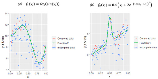
Figure 1.
Scatter plots of both censored data and incomplete response data points over the smooth functions to be estimated by A-splines.
From the data generation procedure given above, the right-censored nonparametric model can be written as follows:
Then, to use censorship information in the estimation process, a synthetic data transformation is done, as in Equation (6). Therefore the final model to be estimated, as given by the simulation experiments, is
In this simulation study, for three sample sizes, three censoring levels, and two functions, 18 configurations are obtained. All the outcomes for the model in Equation (34) under these conditions are given in the following figures and tables.
Table 2 represents the scores of all the evaluation metrics for each of the simulation configurations. The results are inspected from three essential aspects in terms of the estimation performance of the A–spline estimator that are the effects of the sample size, censoring level, and shape of the data. For the first aspect, it can be seen from the table that and decrease when the sample size increases. This can be interpreted as practical proof of the asymptotic convergence that is one of the main purposes of this simulation study. This interpretation is consistent for all censoring levels. The censoring level naturally affects the performance of the estimator contrary to sample size; however, there is a sensitive point, which depends on the reaction of the estimator to variation in the censoring level, which makes this paper significant. If the scores are inspected carefully, it can be clearly seen that there are no huge differences between low and high censoring levels, which can also be seen in the figures given below. This case proves that the A-spline estimator achieves mitigation of the effect of the censoring level on selecting the optimal knot points, as expected. Finally, two different function types are used in this paper. has a shape that is similar to that of a sinus function and is not hard to catch for any smoothing technique. is an almost linear function but has one big peak; this is a challenge for the estimator, especially under censoring. The outcomes in Table 2 demonstrate this. Although the results for are smaller than those for , it can be said that the A-spline estimator shows a satisfactory performance for both datasets.
Table 2.
Variances and biases of , variance of the model , and of for all simulation combinations.
Table 3 represents the comparative outcomes for the introduced estimator modified A-spline and commonly used SS and RS. The best scores are indicated with bold colored text. As can be seen, the results indicate that the modified A-spline estimator shows the best performance from a general perspective. Additionally, as mentioned in the introduction section, RS has smaller MSEs than SS. From here, it can be said that the introduced method gives more satisfying results, which can be explained by its adaptive nature. If Table 3 is inspected carefully, it can be realized that for the results obtained from , the RS method has attractive outcomes when the censoring level is . It is an understandable situation because of the shape of the function.
Table 3.
MSE values for the A-spline, smoothing spline (SS), and regression spline (SS) methods to make comparisons.
Figure 2 aims to show how the modified A-spline estimator behaves when the sample size is exceedingly small, under various censoring levels. It is obvious that the estimation of is easier than that of , which is explained below. Figure 2 shows this more clearly. In addition, it can be said that the method is successful for even extremely small sample sizes (. This is an important contribution of this method for right-censored data because in a medical dataset and especially in clinical observations, many data may frequently be unobtainable.
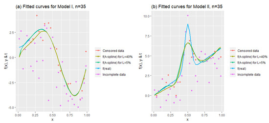
Figure 2.
Fitted curves to see the performance of the estimator for .
Figure 3 presents the effects of sample sizes by keeping the censoring level constant at 20%. Model I was obtained using ; similar fitted curves are obtained for and , and these curves seem to be good representations of the data. This inference is also valid for Model II. Both plots show that the fitted curves successfully model right-censored data.
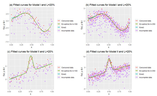
Figure 3.
Fitted curves to see the performance of the estimator for .
Figure 4 demonstrates how the method works under heavy censoring. To that end, fitted curves are shown for a moderate sample size together with the lowest and the highest censoring levels, 5% and 40%. As we expected, the A-spline estimator demonstrates its ability to handle data with zero values obtained by synthetic data transformation, and it can be clearly seen that there is a difference between the two graphs. This inference is also supported by the results in Table 2.
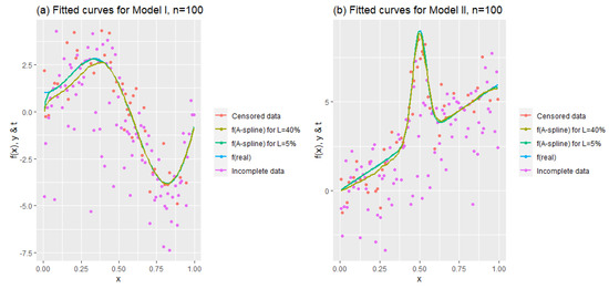
Figure 4.
Fitted curves to observe the quality of the estimates for .
Figure 5 depicts bar plots of the measurement tools for both the estimated A-spline coefficients and the estimated model. In each panel, A1.5%, A1.20%, and A1.40% denote the obtained scores of the evaluation metric for , respectively, for . In a similar manner, A2.5%, A2.20%, and A2.40% represent the scores for and all the censoring levels, and A3.5%, A3.20%, and A3.40% denote the results for for all the censoring levels. The top panels of Figure 5 include bar plots for the bias values. As in Table 2, it can be seen here that the biases for the two models are very similar and, as expected, become smaller in larger samples. The panels in the middle show bar plots for the variances of the coefficients. The plots appear similar for the two models, but, as has been said before, because the estimation of Model II is more difficult than that of Model I, the y-axis is significantly wider in scope. The panel at the bottom is drawn for the values of the estimated model, and it is similar to the variance plots. Essentially, these plots prove that the A-spline estimator can estimate the model by overcoming the effect of censorship in terms of various evaluation metrics.
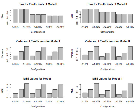
Figure 5.
Bar plots of values for each simulation repetition and their changes under different censoring levels.
5. Real Data Application
This section is prepared to show the performance of the modified A-spline estimator on real right-censored data. The dataset represents data from colon cancer patients in İzmir. The dataset involves the survival times, censoring indicator , and albumin (i.e., the most common protein found in the blood) values of patients. To provide continuity, the logarithms of the survival times are considered as a response variable (), and albumin is taken as a nonparametric covariate (. The right-censored regression model is thus given by
Note, also, that because ’s cannot be used directly in the estimation procedure, they have been replaced by the synthetic responses shown in Equation (6). The model in Equation (36) is thus rewritten as
The dataset contains information for 97 patients to be used for this analysis. However, the records of 32 of these patients are incomplete, containing right-censored observations; the data of the remaining 65 patients are uncensored (deceased). Consequently, in this dataset, the censoring level is . The outcomes calculated for the model in Equation (37) are given the following table and figure.
Table 4 summarizes the performance of the modified A-spline estimator. Note that the values of and are better than the results of Aydın and Yilmaz (2018), who previously used regression splines to model right-censored data. In addition, to provide a healthier comparison, the results of the RS and SS methods are given in the table. As can be seen, the results are pretty similar to the simulation results. Here, A-spline gives the best score, which proves the benefit of the introduce method. Additionally, when the shape of the dataset is inspected from Figure 6, it can be described as having an irregular shape, and it can be seen that this irregularity increases after synthetic data transformation, which is demonstrated by the blue dots in the figure. Despite this challenging case, the A-spline fit seems to represent the data well.
Table 4.
Outcomes for the estimated regression model for colon cancer data.
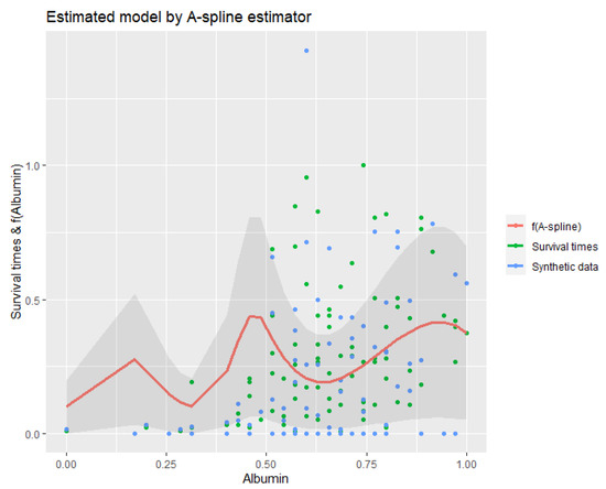
Figure 6.
Estimated model for cancer data by the A-spline estimator.
6. Concluding Remarks
This paper demonstrates that a modified A-spline estimator can be used to estimate the right-censored nonparametric regression model successfully. This is because it uses an adaptive procedure for determining the penalty term and works with only optimum knot points. A simulation study and real data example were carried out to demonstrate the performance of the method, and it can be seen from our findings that the modified A-spline estimator has merit for the estimation of right-censored data.
In the general frame of the numerical examples, incremental changes in the sample size affect the performance of the method, which gives closer results to real observations. This can be seen in Figure 3, Figure 4 and Figure 5. Moreover, changes to the censoring level also influence the goodness of fit, and, as expected, when the censoring level increases, the performance of the method is negatively affected. However, there is an important difference here in terms of the modified A-spline. The main purpose of the usage of this method is to diminish the effect of censorship on the modeling process, and most of our results show that the introduced method achieves this purpose. For an example of these results, see Table 2. In the simulation study, two different function types are used to generate the model. is a cliché pattern of the sinus curve and is not difficult to estimate for any smoothing method. is a little bit more difficult to handle, especially by the smoothing techniques that use all data points as knots. In this paper, it can be seen that for almost all of the simulation configurations, the modified A-spline estimator gives really close values in terms of all evaluation metrics.
The real-world application uses the dataset of colon cancer patients. Their survival times are estimated by using albumin values in their blood. Figure 6 and Table 4 show the outcomes of this study. As mentioned above, our method does a good job despite the unsteadily scattered data points. The confidence interval given by the shaded region in Figure 6 seems wide because synthetic data transformation puts censored points (as zeros) far from the uncensored points. Considering the mentioned properties, it can be said that the modified A-spline estimator can be counted as a robust estimator for right-censored datasets. As a result of this study, we recommend that the modified A-spline estimator is appropriate for modeling clinical datasets.
Author Contributions
Conceptualization, D.A. and S.E.A.; methodology, D.A. and S.E.A.; software, E.Y.; validation, D.A., S.E.A. and E.Y.; formal analysis, E.Y.; investigation, D.A. and E.Y.; resources, D.A.; data curation, E.Y.; writing—original draft preparation, D.A. and E.Y.; writing—review and editing, S.E.A.; visualization, D.A. and E.Y.; supervision, S.E.A.; project administration, S.E.A. All authors have read and agreed to the published version of the manuscript.
Funding
This research received no external funding.
Acknowledgments
Thank the editors and reviewers for their objective assessments.
Conflicts of Interest
The authors declare no conflict of interest.
Appendix A
Appendix A.1. Proof of Lemma 1
Lemma 1 can be proven by using the common independency assumption between and , which is given in Section 1. From that, proof is given as follows:
Thus, proof of Lemma is completed. Note that because of distribution of censoring distribution G is unknown, it is replaced by its Kaplan–Meier estimator that is given in Equation (5).
Appendix A.2. Proof of Theorem 1
The equations given below need to be shown for validation of Theorem 1:
where is the variance of the model defined in (Section 3.1), is a compact set in a metric space and using by Equations (28)–(32), it can be said that
(See [28], for more details).
References
- Stute, W. Consistent Estimation Under Random Censorship When Covariables Are Present. J. Multivar. Anal. 1993, 45, 89–103. [Google Scholar] [CrossRef]
- Kaplan, E.L.; Meier, P. Nonparametric Estimation from Incomplete Observations. J. Am. Stati. Assoc. 1958, 53, 457–481. [Google Scholar]
- Cox, D.R. Regression Models and Life-Tables. J. R. Stat. Soc. Ser. B 1972, 34, 187–202. [Google Scholar] [CrossRef]
- Miller, R.G. Least squares regression with censored data. Biometrika 1976, 63, 449–464. [Google Scholar] [CrossRef]
- Buckley, J.; James, I. Linear regression with censored data. Biometrika 1979, 66, 429–436. [Google Scholar] [CrossRef]
- Miller, R.; Halpern, J. Regression with censored data. Biometrika 1982, 69, 521–531. [Google Scholar]
- Jin, Z.; Lindgren, C.M.; Ying, Z. On least-squares regression with censored data. Biometrika 2006, 93, 147–161. [Google Scholar] [CrossRef]
- Ritov, Y. Estimation in a linear regression model with censored data. Ann. Stat. 1990, 18, 303–328. [Google Scholar] [CrossRef]
- Lai, T.L.; Ying, Z. Estimating a distribution function with truncated and censored data. Ann. Stat. 1991, 19, 417–442. [Google Scholar] [CrossRef]
- Köhler, M.; Máthé, K.; Pinter, M. Prediction from randomly right censored data. J. Multivar. Anal. 2002, 80, 73–100. [Google Scholar] [CrossRef]
- Winter, S. Smoothing Spline Regression Estimates for Randomly Right Censored Data. Ph.D. Thesis, University of Stuttgart, Stuttgart, Germany, 2013. [Google Scholar]
- Aydin, D.; Yilmaz, E. Modified spline regression based on randomly right-censored data: A comparative study. Commun. Stat.-Simul. Comput. 2017, 1–25. [Google Scholar] [CrossRef]
- El Ghouch, A.; van Keilegom, I. Non-parametric regression with dependent censored data. Scand. J. Stat. 2008, 35, 228–247. [Google Scholar] [CrossRef]
- Aydın, D.; Yılmaz, E. Nonparametric regression with randomly right-censored data. Int. J. Math. Comput. Methods 2016, 1, 186–189. [Google Scholar]
- Kim, H.T.; Truong, Y.K. Nonparametric regression estimates with censored data: Local linear smoothers and their applications. Biometrics 1998, 54, 1434–1444. [Google Scholar] [CrossRef]
- Peng, L.; Sun, S. Comparisons between local linear estimator and kernel smooth estimator for a smooth distribution based on MSE under right censoring. Commun. Stat.-Theory Methods 2007, 36, 297–312. [Google Scholar] [CrossRef]
- Koul, H.; Susarla, V.; van Ryzin, J. Regression analysis with randomly right-censored data. Ann. Stat. 1981, 9, 1276–1288. [Google Scholar] [CrossRef]
- Leurgans, S. Linear models, random censoring and synthetic data. Biometrika 1987, 74, 301–309. [Google Scholar] [CrossRef]
- Goepp, V.; Bouaziz, O.; Nuel, G. Spline regression with automatic knot selection. arXiv 2018, arXiv:1808.01770. preprint. [Google Scholar]
- Frommlet, F.; Nuel, G. An adaptive ridge procedure for L0 regularization. PLoS ONE 2016, 11, e0148620. [Google Scholar] [CrossRef]
- Rippe, R.C.A.; Meulman, J.J.; Eilers, P.H.C. Visualization of genomic changes by segmented smoothing using an L0 penalty. PLoS ONE 2012, 7, e38230. [Google Scholar] [CrossRef]
- De Boor, C. A Practical Guide to Splines; Springer: New York, NY, USA, 1978. [Google Scholar]
- Reinsch, C.H. Smoothing by spline functions. Numer. Math. 1967, 10, 177–183. [Google Scholar] [CrossRef]
- Hurvich, C.M.; Simonoff, J.; Tsai, C. Smoothing parameter selection in nonparametric regression using an improved Akaike information criterion. J. R. Stat. Soc. Ser. B 1998, 60, 271–293. [Google Scholar] [CrossRef]
- Eilers, P.H.C.; De Menezes, R.X. Quantile smoothing of array CGH data. Bioinformatics. 2004, 21, 1146–1153. [Google Scholar] [CrossRef] [PubMed]
- Eilers, P.H.; Marx, B.D. Flexible smoothing with B-splines and penalties. Stat. Sci. 1996, 11, 89–121. [Google Scholar] [CrossRef]
- Frank, I.E.; Friedman, J.H. A statistical view of some chemometrics regression tools (with discussions). Technometrics 1993, 35, 109–148. [Google Scholar] [CrossRef]
- Fu, W.; Knight, K. Asymptotics for lasso-type estimators. Ann. Stat. 2000, 28, 1356–1378. [Google Scholar] [CrossRef]
© 2020 by the authors. Licensee MDPI, Basel, Switzerland. This article is an open access article distributed under the terms and conditions of the Creative Commons Attribution (CC BY) license (http://creativecommons.org/licenses/by/4.0/).