Inferring Mechanical Properties of Wire Rods via Transfer Learning Using Pre-Trained Neural Networks

Abstract

The primary objective of this study is to explore how machine learning techniques can be incorporated into the analysis of material deformation. Neural network algorithms are applied to the study of mechanical properties of wire rods subjected to cold plastic deformations. Specifically, this study explores how pre-trained neural networks with appropriate architecture can be exploited to predict apparently distinct but internally related features. Tentative predictions are made by observing only an insignificant cropped fraction of the material’s profile. The neural network models are trained and calibrated using 6400 image fractions with a resolution of $120\times 90$ pixels. Different architectures are developed with a focus on two particular aspects. Firstly, different possible architectures are compared, particularly between multi-output and multi-label convolutional neural networks (CNNs). Moreover, a hybrid model is employed, essentially a conjunction of a CNN with a multi-layer perceptron (MLP). The neural network’s input constitutes combined numerical and visual data, and its architecture primarily consists of seven dense layers and eight convolutional layers. By proper calibration and fine-tuning, observed improvements over the standard CNN models are reflected by good training and test accuracies in order to predict the material’s mechanical properties, with efficiency demonstrated by the loss function’s rapid convergence. Secondly, the role of the pre-training process is investigated. The obtained CNN-MLP model can inherit the learning from a pre-trained multi-label CNN, initially developed for distinct features such as localization and number of passes. It is demonstrated that the pre-training effectively accelerates the learning process for the target feature. Therefore, it is concluded that appropriate architecture design and pre-training are essential for applying machine learning techniques to realistic problems.

1. Introduction

With the escalating global drive towards environmental sustainability and energy efficiency, industries like automotive, aerospace, and construction are seeking innovative solutions that can cater to the fabrication of lightweight components. One path to this goal is the adoption of wire with a decrease in cross-sectional area, which allows for weight reduction and ensures judicious utilization of metal resources [1]. Steel wire rods, a key element in contemporary industrial applications, span a broad spectrum of applications. These applications often stipulate rigorous standards for dimensional accuracy and mechanical properties. Moreover, the gamut of wire sizes required is staggeringly diverse, ranging from millimeters to extensive lengths [2].

Regarding the manufacturing sector, processes such as roller cassette die deformation, drawing, and swaging are pivotal in wire production. Subsequently, the inherent mechanical properties of diverse materials undeniably govern their adaptability to these processes. Moreover, a profound understanding and optimization of these properties are indispensable to foster the fabrication of premier, lightweight components. The roller die cassette stands out among these processes and is an innovative substitute for conventional wire-drawing dies. This technique is characterized by a two-stage deformation where a wire rod undergoes deformation through two sets of rolls. The initial set imparts an oval shape, possibly inducing finning, while the subsequent set reinstates the circular configuration, as illustrated in Figure 1. Empirical investigations vouch for its merits in enhancing productivity and product caliber [1,3]. Delving deeper into its mechanical nuances, extensive research [3,4,5,6] has been carried out. Recent studies have further expanded the understanding of these processes. El Amine et al. [3] conducted an experimental comparison, revealing that roller dies improved surface finish by approximately 40% but increased wire temperature. Yoshida et al. [7] investigated tilting in fine wire roller drawing, identifying critical parameters to prevent defects in wires as small as 200 μm. A comparative analysis by Burdek et al. [8] using the finite element method and numerical simulations showed that roller dies reduced drawing force by 25% while improving dimensional accuracy for high-carbon steels. Advancements in titanium wire drawing [9] demonstrated a 30% reduction in friction when using roller dies for Ti-6Al-4V processing. These studies collectively highlight the ongoing improvements in roller die technology, particularly in surface quality, reduced friction, and the integration of advanced modeling techniques for process optimization. In general, wires crafted via roller die manifest reduced tensile and yield strengths compared to conventional methods. However, this technique compensates with operational efficiencies, such as diminished power consumption and a heightened deformation ratio per pass, while avoiding central cracks—a common flaw in traditional wire drawing.

However, while prior investigations have illuminated the roller die cassette’s myriad facets, there remains uncharted territory that warrants exploration. Pertinent queries encompass understanding the reduction in cross section, discerning the repercussions of consecutive passes, and examining localized variations in the cross-sectional area of the processed wire rod. Such localized strains potentially induce inconsistencies across the wire cross section, precipitating disparities in material hardening, structural composition, texture, and stress residue distribution. This heterogeneous nature of the wire further complicates evaluations of the deformation ratios at ambient temperatures, the texture of the cross-sectional profile, and the tensile properties inherent to the roller die drawing. An avenue conspicuously underrepresented in the current literature is employing machine learning (ML) [10] and automated optimization to address these multifaceted challenges.

As a subfield of artificial intelligence (AI), ML revolves around developing mathematical models that learn from data. Rather than being pre-programmed, these models evolve from the insights they derive from training data. Their applications have permeated numerous domains, from medicine to computer vision, proving particularly potent where traditional methodologies are less efficient. Notable progress in ML relates to pattern recognition, especially with convolutional neural networks (CNNs) [10], which draw inspiration from biological neural connections. The algorithm is the primary choice for image analysis owing to its unparalleled efficiency and effectiveness. Outperforming traditional techniques like polynomial fits via Lagrange cardinal functions, CNNs excel in image processing, finding applications in radiology [11,12,13,14,15], pattern recognition [16,17], tracking [18,19,20], and, particularly, material science [21,22,23,24,25]. Nevertheless, the area of wire plastic deformation remains underexplored mainly in the literature. Recently, a CNN was applied to a binary classification problem to discriminate between different wire deformation methods [26]. The approach was further developed to simultaneously identify different features [27] using a multi-output network composed of two primarily separated components. Most recently, Liang et al. [28] applied machine learning techniques to analyze wire rolling processes, achieving 92% accuracy in predicting cross-sectional profile deviations. These studies demonstrated the potential of ML techniques in analyzing wire deformation processes. Nonetheless, the efforts mentioned above are primarily associated with the information of the underlying process but not the mechanical properties of the resulting material, whereas the latter are of practical significance.

The present study is primarily motivated by the fact that ML techniques have not been widely applied to this specific area, and existing studies [29,30,31,32] have mainly been qualitative rather than based on quantitative image processing algorithms. Therefore, the objective of this study is quantitative, and the metric is in terms of the prediction accuracy rate of the neural network and the loss function. Specifically, by employing various architectures as well as pre-training and fine-tuning approaches, analysis of the microstructure of the material is performed with an emphasis on extracting the tensile strength of the resulting wire rod material. The datasets utilized in this study consist primarily of light microscopy images of materials exposed to various cold deformation processes. Comparison is performed on the respective performance using different architectures, including the multi-label and multi-output CNN and a hybrid (CNN and multi-layer perceptron) CNN-MLP model. The CNN architecture is employed for its effectiveness in image analysis, while the MLP is preferred for data processing. Moreover, the effectiveness of transfer learning [33] via a pre-trained learning process is demonstrated to extract information on the tensile strength of the material based on apparently distinct features. Remarkably, a CNN trained on a minimal cropped segment of the cross-sectional profile of the material is shown to be capable of extracting valuable information about the material.

Figure 1. The configuration of the “3+3” roller die cassette system. Extracted from Ref. [34].

Figure 1. The configuration of the “3+3” roller die cassette system. Extracted from Ref. [34].

2. Experimental Setup and Measurements

This section is a brief review of the experimental setup employed in the present study, and additional details can be found in [27]. The experiment utilized a wire rod with a diameter of 6.65 mm, manufactured by rolling commercial AISI 1008 carbon steel. The chemical composition is listed in

Table 1. Chemical composition (%) of AISI 1008 steel wire rod (Ø6.65 mm) [26].

C	Mn	P	S	Si	B
0.08	0.45	0.018	0.029	0.095	0.0002

. The wire rod was subjected to a chemical pickling procedure using an aqueous solution of sulfuric acid and then coated with zinc phosphate, which acted as a carrier for the lubricant. The wire rod underwent cold deformation using a multi-pass roller die cassette drawing machine running at 1.6 ${\mathrm{ms}}^{-1}$. Several specimens underwent this procedure.

The cold wire rolling tests employed a commercially available microcassette roller die cassette consisting of two sets of three rollers. The experimental layout can be observed in Figure 1. A detailed overview of the pass schedules and the resulting mechanical properties can be found in

Table 2. Dimensions and mechanical attributes of AISI 1008 steel wire rods subjected to varying roller die drawing passes. The cumulative reduction amounted to 59.73%. Values rounded to reflect measurement precision.

Wire Rod		Reduction	Vickers Microhardness		Tensile Strength
Pass	(mm)	(%)	Cross-Sectional	Longitudinal	(MPa)
0	Ø6.65	0.00	159	145	438
1	Ø5.63	28.32	236	249	634
2	Ø4.88	24.86	278	272	764
3	Ø4.22	25.22	279	280	795

. Specifically, Vickers microhardness testing was performed using a Buehler Micromet 2004 tester (Buehler, Lake Bluff, IL, USA) following the ASTM E384-17 standard [35]. A load of 100 gf (0.9807 N) was applied for 15 s. Measurements were taken at five points along both the cross-sectional and longitudinal axes of the samples, maintaining a minimum distance of 0.3 mm from the edges. This procedure was carried out for wire samples from all three drawing passes (⌀6.5 mm to ⌀4.22 mm). For the uniaxial tensile tests, the ASTM E8/E8M-21 standard [36] was adhered to using a Shimadzu AG-Xplus 250 kN universal testing machine (Shimadzu Corporation, Kyoto, Japan). The specimens had diameters ranging from ⌀6.5 mm to ⌀4.22 mm, with a gauge length of 100 mm (following the $L_0=4D$ rule). Tests were conducted at room temperature (23 ± 1 °C) with a crosshead speed of 0.5 mm/min, corresponding to an initial strain rate of 0.000083 ${\mathrm{s}}^{-1}$. The recorded microhardness and tensile strength are calculated as an average of three specimens and presented in Table 2. The testing equipment was regularly calibrated using NIST-traceable references, and all measurements were performed in a controlled environment as per standard guidelines.

Individual passes were subjected to cross-sectional decrease measurements. A decrease in the cross-sectional area of 59.73% was found during wire rolling, as indicated in Table 2. These processes have a significant impact on the microstructure of the material. Before conducting the microstructure study, the necessary metallographic preparations were performed according to conventional procedures. To reveal the steel microstructure, samples were etched using a 3% Nital solution (3% nitric acid in ethanol). This etchant was chosen for its effectiveness in revealing martensitic structures and ferrite grain boundaries in low-carbon and low-alloy steels, which is crucial for analyzing the microstructural changes resulting from the wire drawing process. The truncated specimen was prepared by embedding, grinding, and polishing transverse sections. In particular, the samples were embedded in epoxy resin at room temperature to maintain cross-sectional integrity. Transverse sections were cut using a precision blade under coolant to minimize thermal artifacts. Mechanical grinding was performed using SiC sheets with increasing grit numbers of 180, 280, 320, 400, 600, and 1200 mesh. Final polishing used a 1 μm diamond suspension to achieve a mirror finish. The profiles were examined using a Leica Light Microscope (Leica Microsystems GmbH, Wetzlar, Germany) model DM 4000 M, to determine the effects of deformation processes on the microstructure of the material. Illustrations of post-rolling cross-sectional profiles can be found, for instance, in Figure 3 of [27].

Preliminary qualitative studies indicated variations in the texture of the cross-sectional wire profiles across different deformation stages, as well as the properties of the border and center regions [3,37]. In what follows, we seek a more comprehensive, quantitative understanding, focusing on leveraging ML techniques to investigate the microstructures and mechanical properties of the obtained material.

3. Model Calibration and Data Augmentation

This section discusses in detail the datasets and the specific architectures of the neural network models used in this paper. The models explored in this study consist of a hybrid CNN-MLP model, a multi-label CNN, and a multi-output CNN, as well as their variations. Furthermore, the performed data augmentations and model calibrations are discussed. Specifically, details on the datasets are discussed in Section 3.1 and the data augmentations in Section 3.2. In Section 3.3, model calibrations are performed, and the results are presented.

3.1. Datasets

The experimentally measured cross-sectional profiles and features furnish two datasets. The image dataset is implemented by dividing the original profiles of the processed material into smaller images. These cropped images are subsequently divided into separate datasets for training, validation, and testing. In this study, a total of 6400 image segments are used, with 5113 randomly chosen for training, 1279 allocated for validation, and the rest assigned to the test set. As explained further below, k-fold cross-validation is also conducted to ensure the reliability of the findings. In addition to the images, a numerical dataset is also established, which contains information on the localization and number of passes associated with the material.

These datasets are fed to neural networks of two main types: CNN and MLP. The CNN branch receives the image data as input and classifies them through convolutional, pooling, batch normalization, dropout, flattening, and dense layers. The final output of the classification is a four-element array that carries the information on the mechanical properties. In the first and second rows of Figure 2, eight randomly cropped images utilized for the training set are displayed. The features of interest include the process parameters and measured mechanical properties, which are pegged to four different values of tensile strength. The numerical dataset consists of information on the location and number of passes, which are stored as binary and integer variables. The MLP branch’s input is the numerical dataset, a two-element array containing the process parameters of the underlying cross-sectional profiles. The data are processed via dense and dropout layers, leading to a four-element output representing the tensile strength associated with the cross-sectional surface.

3.2. Data Augmentation

Augmentations are used to generate new images from existing ones, increasing the size of the training dataset. Similarly to a previous study [26], geometric transformations are applied, such as rotation and flipping, to the existing image profiles, resulting in extra data that impulsively push the model toward a better generalization. As discussed below, the options for “fill mode”, consisting of the possible forms to fill the excess derived from the rotation and flipping transformations, are explored. Out of various possibilities, the color pixel range normalization—specifically the “rescale” method—is deliberately applied to stop the network from easily identifying patterns based on color depth. A selection of augmentations (i–k) applied to the original image (a) is illustrated in the third row of Figure 2. The final image (l) demonstrates the cumulative effect when all augmentations are applied concurrently.

3.3. Network Architecture and Calibration Process

The model calibration is performed to determine favorable specifications. As an illustration, the primary focus is on the hybrid CNN-MLP model. Employing a similar strategy, this process is performed for the remaining models when it is applies.

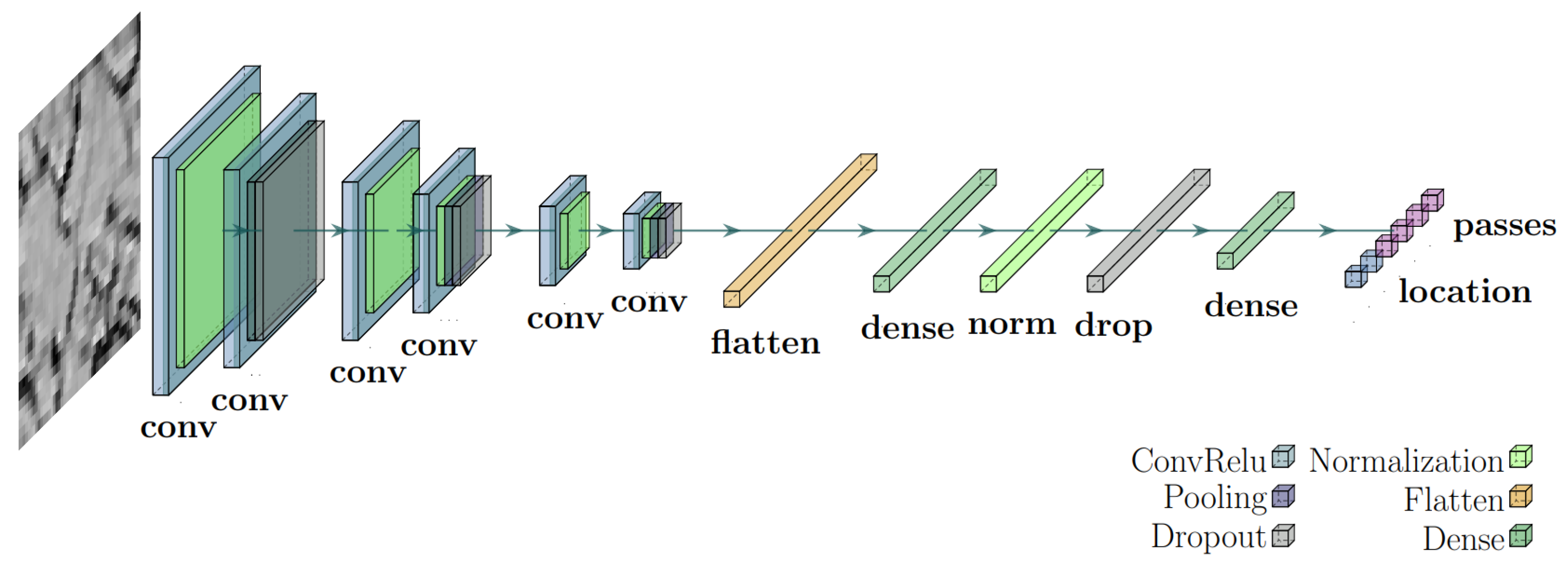
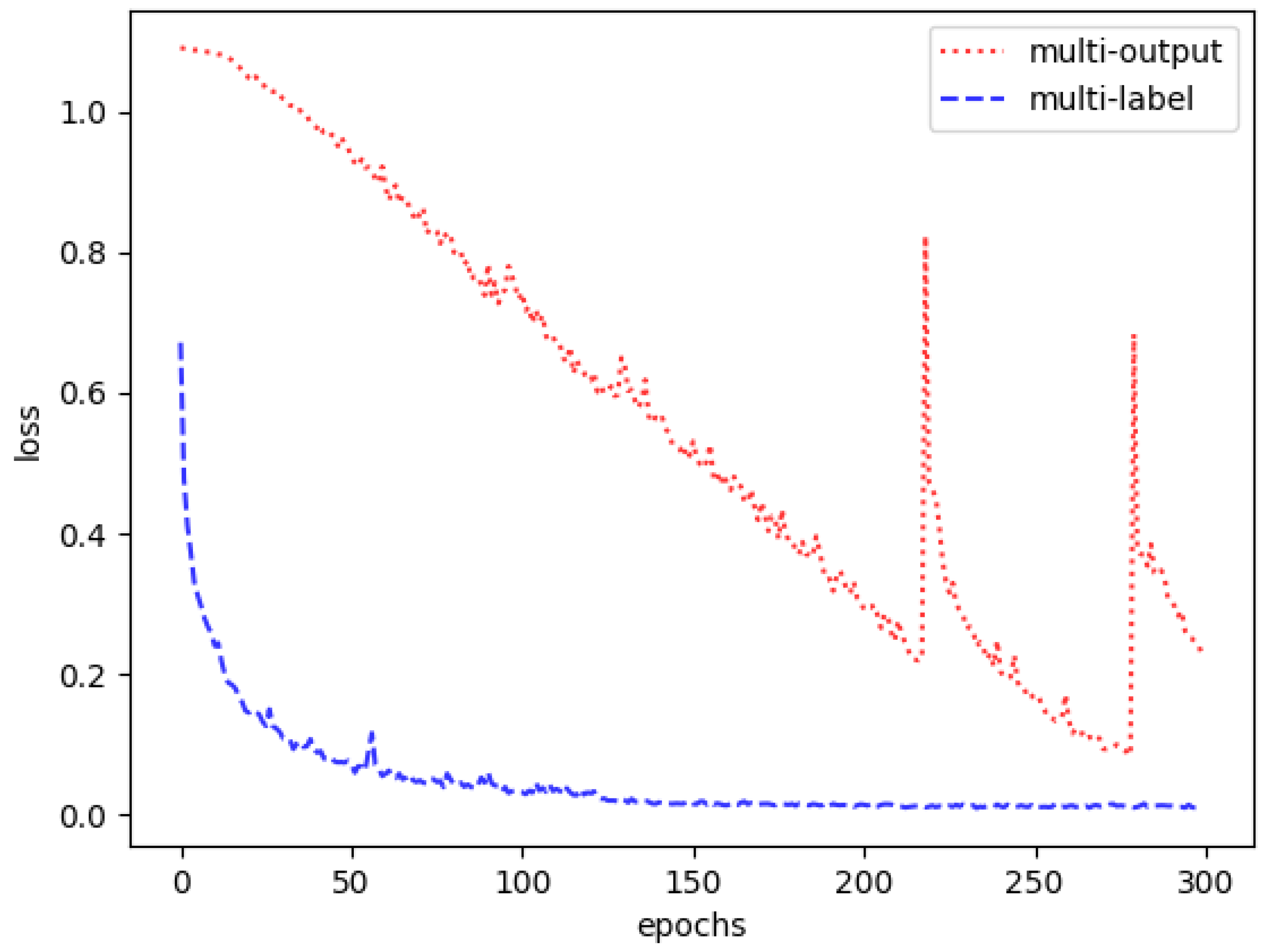
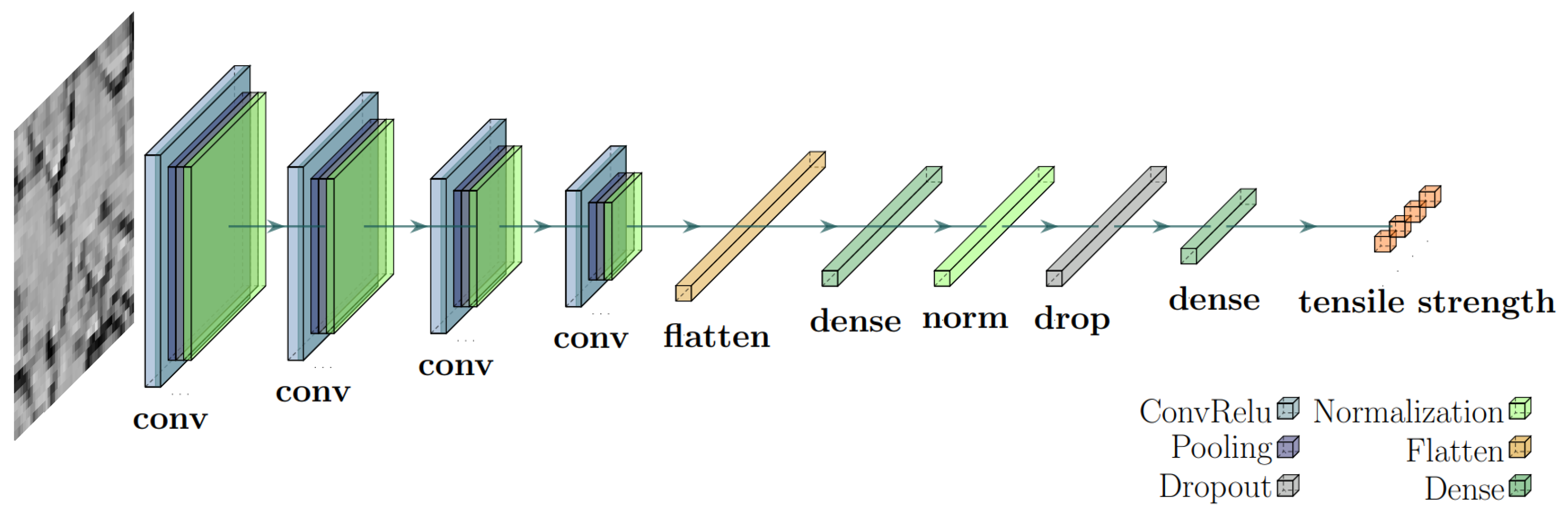
The architectures of the models are presented in Figure 3, Figure 4, Figure 5 and Figure 6. The multi-output CNN was employed in [27] to explore the process parameters, such as the number of passes applied to the material. As shown in Figure 3, it consists of largely independent networks, individually dedicated to distinct features. The multi-label CNN is closely related and is often an alternative approach to the multi-output architecture. The main difficulty of employing the multi-label architecture for such a task is that a few different features are mutually exclusive. Therefore, a straightforward application of the multi-label network is not feasible as it might cause the network to predict some properties that are not physically plausible simultaneously. To circumvent such a difficulty, a filter layer is added at the network’s output that guarantees that only one feature out of a collection of mutually exclusive ones is selected based on its “rank”. A schematic layout of the multi-label CNN is given in Figure 4. A more detailed comparison between the multi-output and multi-label CNNs is developed further in Section 4.1.

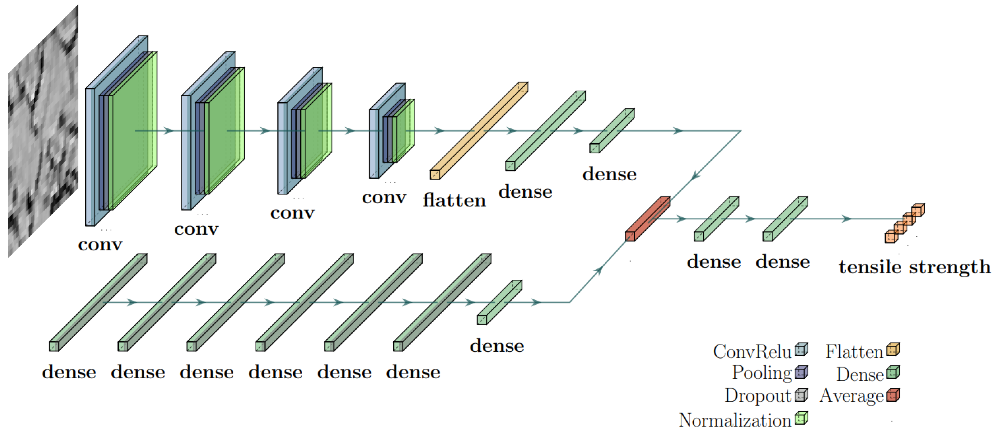
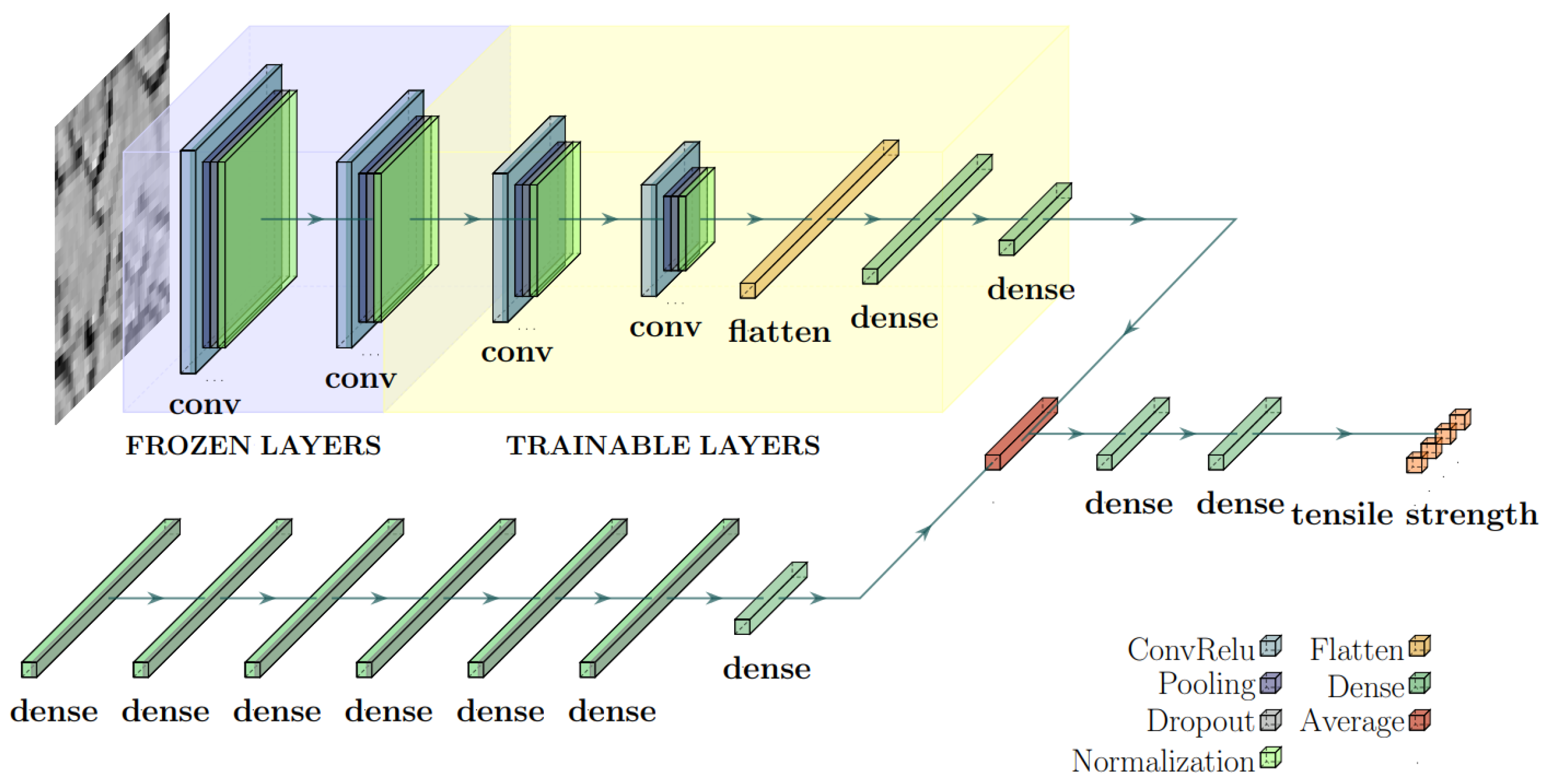
The hybrid model proposed in [38] was applied, which combines a CNN with a long short-term memory (LSTM) network, a recurrent neural network variant. However, this approach is designed for processing temporal or sequential data, which is unsuitable since the input comprises process parameters that are fundamentally different in nature from ordered sequences. To address this, the LSTM is replaced with an MLP. This neural network’s input constitutes both image and numerical data. The image input is identical to the multi-output and multi-label CNNs described above. The numerical input consists of some of the material’s features that are seemingly irrelevant to the features of interest. The CNN’s architecture primarily consists of a few intercalated dense and convolutional layers, followed by a few flattening and dense layers, which are to be determined by the calibration process. A couple of dense layers furnish the MLP. The two networks are then merged by averaging before passing through two dense layers. The schematic architecture of the hybrid model is shown in Figure 5. Lastly, this study also utilizes a multi-class CNN model, which possesses primarily identical architecture to the CNN sector of the hybrid model. As discussed in Section 4.3, it is introduced to compare the effectiveness between different models.

As an illustration, the calibration process of the hybrid model, which emphasizes the CNN sector, is discussed in the following. The architecture is denoted as a ratio of the shape and weight of the convolutional layer’s output to the number of convolutional kernel instances, represented as “(size, weight)/no. kernel”. The intermediate pooling and fully connected layers are assumed to be present but not specifically quantified. In particular, the CNN sector’s architecture within the model is denoted as

$$\left[(S_1,W_1)/F_1,(S_2,W_2)/F_2,\cdots ,(S_N,W_N)/F_N\right],$$

(1)

where N is the total number of convolutional layers. The following aspects are analyzed: batch size, data augmentation “fill mode”, architecture in terms of the number of dense and convolutional layers, optimizer schemes, and the ReduceLROnPlateau callback application and its inherent parameters. Unless specified, the calculations are carried out by using the following given CNN layout:

$$\left[(120,90)/32,(57,42)/32,(26,19)/64,(11,7)/64\right].$$

(2)

Table 3. The calibration regarding different options for batch size with a given layout shown in Equation (2) for 100 epochs.

Batch Size	16	32	64	128
training accuracy	99.65%	99.94%	99.90%	99.80%
training loss	0.0136	0.0028	0.0048	0.006
validation accuracy	98.91%	81.55%	99.92%	69.43%
validation loss	0.0392	0.3892	0.0054	1.098

displays the results for both training and validation datasets regarding different options of batch sizes. Calculations are carried out for a given layout shown in Equation (2) with 100 epochs with different batch sizes of 16, 32, 64, and 128. As shown below, the 64-batch size produces the best results among the options tested; it gives the highest accuracies while showing reasonably consistent values for the training and validation results.

Various data augmentation techniques are utilized, as shown in the third row of Figure 2. An analysis of the effects of various options related to the fill mode are shown in

Table 4. The calibration regarding different options of fill mode with a given layout shown in Equation (2) for 100 epochs.

Fill Mode	Nearest	Constant	Reflect	Wrap
training accuracy	99.88%	99.90%	99.86%	99.74%
training loss	0.0053	0.0048	0.0061	0.0109
validation accuracy	99.84%	99.92%	53.79%	73.49%
validation loss	0.0167	0.0054	1.207	1.553

, which determines the specific recipe used to top up the excess space in an image after the augmentation. Although it might seem that the “constant”, “nearest”, or “reflect” modes have little impact on the texture information of the profiles, practical results show otherwise. Specifically, the “constant” mode provides marginally improved performance in terms of training and validation accuracies for the model, as evidenced in Table 4.

The architecture of the hybrid model is analyzed and presented in

Table 5. The calibration of the CNN sector of the network regarding different layouts as defined in the text.

CNN Layout	1	2	3
training accuracy	99.94%	99.68%	99.90%
training loss	0.0045	0.0119	0.0048
validation accuracy	99.92%	100.00%	99.92%
validation loss	0.0057	$6.855\times {10}^{-4}$	0.0054

and

Table 6. The calibration of the MLP sector of the network regarding different numbers of dense layers.

No. of Dense Layers	2	4	6
training accuracy	99.84%	99.78%	99.90%
training loss	0.0066	0.0083	0.0048
validation accuracy	100.00%	99.77%	99.92%
validation loss	0.0025	0.01099	0.0054

. The CNN sector shows the resultant accuracies by exploring different architectures in terms of different numbers of convolutional and dense layers. Specifically, the following three different layouts are explored:

$$\begin{array}{cc}\hfill \mathrm{Layout}1:& \left[\right(120,90)/32,(57,42)/32].\hfill \\ \hfill \mathrm{Layout}2:& \left[\right(120,90)/32,(57,42)/32,(26,19)/64].\hfill \\ \hfill \mathrm{Layout}3:& \left[\right(120,90)/32,(57,42)/32,(26,19)/64,(11,7)/64].\hfill \end{array}$$

(3)

These architectures utilize alternating filter sizes of $3\times 3$ and $2\times 2$ pixels and are trained over 100 epochs with a batch size of $(25,11)$ and an “Adam” optimizer. Table 5 illustrates how the network’s sensitivity varies with the number of convolutional layers across different architectures. Generally, increasing the number of layers enhances performance, though the improvement is incremental. A network with just three layers and a well-designed architecture can still achieve decent precision. When more advanced architectures are used, training and validation accuracies tend to stabilize, showing marginal gains.

Regarding the MLP sector, in Table 6, the results for different architectures are presented. The calculations use two, four, and six dense layers while keeping intact the CNN’s architecture shown in Equation (2). It is noted that a reasonable number of dense layers is already sufficient. As the number of layers increases further, the network performance increases slightly. The above calibration determines the architecture of the CNN-MLP model, whose detailed layout is presented in

Table 7. The detailed layout of the hybrid CNN-MLP model determined through the calibration process described in the text.

Hybrid Model
CNN Branch		MLP Branch
Layer	Dimensions	Layer	Dimensions
Input Layer	(None, 120, 90, 1)	-	-
Conv2D Layer 1	(None, 118, 88, 32)	-	-
MaxPooling Layer 1	(None, 59, 44, 32)	-	-
Dropout 1	(None, 59, 44, 32)	-	-
BatchNormalization 1	(None, 59, 44, 32)	-	-
Conv2D Layer 2	(None, 57, 42, 32)	-	-
MaxPooling Layer 2	(None, 28, 21, 32)	Input Layer	(None, 2)
Dropout 2	(None, 28, 21, 32)	Dense Layer 1	(None, 40)
BatchNormalization 2	(None, 28, 21, 32)	Dropout 1	(None, 40)
Conv2D Layer 3	(None, 26, 19, 64)	Dense Layer 2	(None, 40)
MaxPooling Layer 3	(None, 13, 9, 64)	Dropout 2	(None, 40)
Dropout 3	(None, 13, 9, 64)	Dense Layer 3	(None, 40)
BatchNormalization 3	(None, 13, 9, 64)	Dropout 3	(None, 40)
Conv2D Layer 4	(None, 11, 7, 64)	Dense Layer 4	(None, 40)
MaxPooling Layer 4	(None, 5, 3, 64)	Dropout 4	(None, 40)
Dropout 4	(None, 5, 3, 64)	Dense Layer 5	(None, 40)
BatchNormalization 4	(None, 5, 3, 64)	Dropout 5	(None, 40)
Flatten Layer	(None, 960)	Dense Layer 6	(None, 40)
Dense Layer 1	(None, 128)	Dropout 6	(None, 40)
Dense Layer 2	(None, 4)	Dense Layer 7	(None, 4)
Average Layer: (None, 4)
Merged Dense Layer 1: (None, 4)
Merged Dense Layer 2: (None, 4)

.

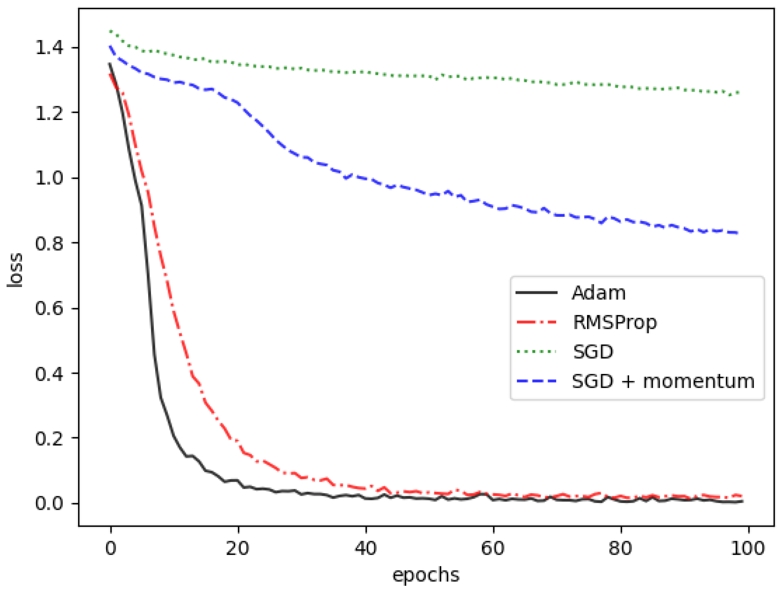
In terms of the loss function, “sparse categorical cross-entropy” was utilized, which combines a Softmax activation plus a cross-entropy loss. Several options for the optimizers were evaluated, including the adaptive learning rate optimization algorithm (Adam), root mean squared propagation (RMSprop), standard stochastic gradient descent (SGD), and a standard stochastic gradient descent with a variation in the “momentum” parameter (SGD + momentum). The outcomes of these four optimizer options are illustrated in Figure 7 and

Table 8. The convergence of the network’s training and validation curves using different optimizers.

Optimizer	Adam	RMSprop	SGD	SGD + Momentum
training accuracy	99.90%	99.39%	38.17%	63.72%
training loss	0.0048	0.0206	1.261	0.0824
validation accuracy	99.92%	45.90%	27.37%	46.99%
validation loss	0.0054	4.1086	1.3791	1.564

. A review of Table 8 reveals that “Adam” outperforms the other optimizers. Furthermore, Figure 7 demonstrates that “Adam” achieves quicker convergence compared to the alternatives, making it the preferred choice for the current CNN architectures.

Lastly, the outcome indicates a certain degree of overfitting, as the model performs significantly better in training than in validation. In this regard, ReduceLROnPlateau callback was employed to minimize overfitting. The option monitors one specific quantity as a metric and reduces the learning rate when the metric stops improving. In this aspect, the validation loss values were chosen as the monitor quantity. As a result, the model’s learning rate would be reduced as the validation performance starts decreasing considerably. The callback implementation effectively decelerates the learning process and subsequently improves the model’s convergence among the train and validation datasets. In particular, a parameter of the ReduceLROnPlateau tool called “patience” plays a crucial role. This parameter is responsible for assigning the maximum number of epochs, inclusively, for the case where no improvement is observed for the monitored metric until the learning rate is reduced. As shown in

Table 9. Model performance regarding different values of patience in the ReduceLROnPlateau callback with the given layout shown in Equation (2) for 100 epochs.

Patience	10	15	20	25
training accuracy	97.27%	99.29%	99.94%	99.76%
training loss	0.08	0.0274	0.0032	0.0073
validation accuracy	50.90%	49.88%	100.00%	99.92%
validation loss	1.931	3.197	$8.7625\times {10}^{-4}$	0.0046

, one perceives that this parameter is vital for the calibration algorithm to detect the correct moment when the model stops learning. This allows the training and validation to converge at the highest accuracies, while the losses are essentially minimized. Moreover, the robustness of the results was confirmed through a k-fold cross-validation, which considers different separations of the training and validation datasets. The results are presented in

Table 10. K-fold cross-validation performance comparison (vs. Table 9). Results are obtained using patience of 25 with layout shown in Equation (2) over 150 epochs.

Fold	1	2	3	4
training accuracy	99.77%	99.92%	99.97%	99.92%
training loss	0.0097	0.0027	0.0009	0.0023
validation accuracy	99.84%	99.99%	99.61%	98.20%
validation loss	0.0239	0.0021	0.0075	0.0454

.

These results indicate that reasonable and consistent accuracy is achieved for the proposed model. The models utilized are robust enough to effectively detect critical patterns within the data. Although there were some cases of misidentification, the accuracy levels demonstrate the approach’s promise for real-world applications. However, it is worth noting that factors such as input data quality, task complexity, and the suitability of the model design can impact performance. Thus, while the results are promising, additional testing and fine-tuning might be required to guarantee sustained high accuracy when tackling new or more challenging datasets. Given the model calibration, the comparison of the efficiency of different network architectures and the effect of the pre-training process are discussed in the next section.

4. Further Analysis of the Architecture and Pre-Training Process

This section further elaborates on two specific aspects. First, we explore the differences due to the different architectural designs and, in particular, we compare the multi-output and multi-label CNNs in Section 4.1. As discussed in the Introduction, an objective of this study is to employ transfer learning [33] concepts to develop an efficient model to predict the mechanical properties of the material. Specifically, two training processes with and without the pre-training process are elaborated on, based on the specific network parameters pre-trained on the remaining features of the material developed recently in [27]. Section 4.2 discusses the transfer learning process implemented for the hybrid model discussed above. Finally, Section 4.3 concludes by presenting the results for all the approaches involved in the present study.

4.1. Multi-Output vs. Multi-Label Architecture

As mentioned in Section 3.3, there are two similar but different candidates for the architecture design when dealing with multiple features. The first is the multi-output CNN utilized in [27], for which two characteristics, namely, the position of the cropped profile and the number of passes, are mainly trained separately to provide a multi-output architecture. An alternative is to adopt a multi-label CNN. Adopting a multi-label approach may not seem viable. This is essential because in most scenarios where a multi-label approach is applied, the labels are not necessarily mutually exclusive by definition. It is different in this case. For example, an observed material must have passed the deformation process a well-defined number of times; it cannot be once and twice simultaneously. Therefore, a multi-output CNN was adopted in [27]. However, it is argued that using multi-label architecture for the present scenario is also feasible. As explained above, an additional filter layer may be introduced that picks out only one of the mutually exclusive features. This can be implemented by choosing the feature with the highest rank. As demonstrated in the following, this particular algorithm is more efficient because it increases the accuracy and convergence rate in the network’s training and validation processes. This is because the underlying architecture allows the neurons from different layers to interact more efficiently, resulting in better training and validation performances.

The multi-label CNN developed in the present study can be seen as an improved version of its multi-output counterpart. It consists of a unified structure that simultaneously processes six features, the labels. Specifically, two of them indicate the cropped profile’s position, center or peripheral, and four of them are related to the number of passes: zero (unprocessed), once, twice, and three times. Each label is considered a Bernoulli variable, and the binary cross-entropy loss function is used. Therefore, the network’s output is a collection of binary classification predictions for all six labels.

The above setup does not prevent mutually exclusive features from being selected simultaneously. To proceed, the labels are divided into subsets consisting of all mutually exclusive labels and the model assigns a “ranking” to each member of the subset based on its respective weight in the loss function in reverse order. It is possible given that each label always and only belongs to one of the subsets. Subsequently, an additional layer is introduced that only picks out the label of the highest ranking from each subset and ignores the remaining ones. As it turns out, such an architecture offers superior accuracy rates to its multi-output counterpart. The model calibration and validation processes are carried out in a fashion similar to that discussed above in Section 3.3. The data augmentation indicates that the highest values for accuracy are found with the “constant” fill mode. The best performance occurs for a batch size of 64 using the layout of

$$\left[\right(120,90)/32,(57,42)/32,(26,19)/64,(11,7)/64,(26,19)/128,(11,7)/128],$$

(4)

and the best optimizer is Adam. For the training and validation processes, the ReduceLROnPlateau callback parameter “patience” is explored, and the results are shown in

Table 11. Model performance regarding different values of patience in the ReduceLROnPlateau callback with the given layout shown in Equation (4) for 100 epochs.

Patience	10	15	20	25
training accuracy	98.10%	96.77%	96.97%	98.70%
training loss	0.0528	0.0865	0.0783	0.0376
validation accuracy	98.47%	96.33%	97.33%	98.73%
validation loss	0.0413	0.0941	0.0691	0.0347

.

The multi-label CNN achieved a precision of 98.70% and 98.73%, respectively, for training and validation. As a comparison, in a previous study [27], using a multi-output CNN of roughly the same size, the training and validation precision values of 98.9% and 79.4% for the localization and 94.1% and 78.1% for the number of passes were reported.Therefore, when compared to the performance of the multi-output counterpart, the improvement is apparent. The convergence rate of the loss functions of the two approaches is also studied. The numerical results are presented in Figure 8. As shown in Figure 8, the convergence for the multi-label CNN is much faster while achieving an overall superior accuracy.

4.2. Effectiveness of the Pre-Training Process for the Hybrid CNN-MLP Model

In this subsection, one aim is to explore the effectiveness of the pre-training process. Again, the hybrid CNN-MLP model is utilized. Instead of training the model from scratch, as in Section 3.3, we elaborate on a transfer learning process to analyze the material’s tensile strength. Specifically, the initial parameters of the model’s CNN section are defined by the weights and bias of the process parameters extracted from the pre-trained multi-label CNN, developed in the last subsection for process parameters such as localization and number of passes. These model parameters carry information on rather distinct features. As shown below, the obtained CNN-MLP model inherits the learning from the multi-label CNN and effectively speeds up the learning process for the target feature of tensile strength.

To highlight the pre-training process, the training and validation were performed while freezing specific pre-trained layers in the CNN sector of the hybrid model. In other words, some layers are not trainable as their weights and biases are entirely governed by the multi-label CNN. Conversely, the model parameters in the MLP sector are always treated as free during the training and validation processes. As illustrated in Figure 9, we consider one, two, and three unfrozen layers in the CNN layout. The results of the model’s performance are shown in

Table 12. The performance of the hybrid model for different pre-training options where different numbers of layers of the multi-label CNN layout are frozen. The calculations are carried out using 100 epochs.

Unfrozen Layers	1	2	3
training accuracy	99.76%	99.94%	99.86%
training loss	0.0083	0.0034	0.0050
validation accuracy	78.42%	100.00%	99.84%
validation loss	0.7035	0.0042	0.0184

.

It is observed in Table 12 that the best performance is achieved by unfreezing two layers with the pre-trained parameters. This is understandable, as these parameters are extracted from a multi-label CNN trained initially on the general characteristics of the profiles but mainly irrelevant to the feature of interest. On the one hand, if a significant fraction of the network is frozen to the pre-trained parameters, it will significantly constrain the freedom and subsequently undermine the underlying architecture’s performance. On the other hand, if only a small fraction of the network is frozen, the information from the pre-trained network might not be effectively used. An extreme case of the latter is to train the network from scratch, as carried out earlier in Section 3.3. By balancing the two scenarios, the model turns out to be the most effective when approximately half of the pre-trained network’s parameters are assigned to be free.

4.3. Fine-Tuning and a Comparison Between the Models

Following the training of the hybrid CNN-MLP model, where some of the pre-trained layers are frozen, fine-tuning is now introduced. This process consists of training the model again by relaxing all the parameters of the entire model. Only minor adjustments to the weights and bias and the corresponding improvement in accuracy rate are expected in this last stage.

Finally, we present a comparison of the performance of the proposed models in this study. The results are shown in

Table 13. A comparison of the accuracy rates among the approaches employed in the present study.

Model	Target Features	Training Accuracy	Validation Accuracy	Training Loss	Validation Loss
multi-output CNN	process parameters	98.9% and 94.1%	79.4% and 78.1%	0.0001	0.0108
multi-label CNN	process parameters	98.82%	99.05%	0.0333	0.0299
multi-class CNN	tensile strength	93.59%	70.87%	0.1767	1.2199
hybrid CNN-MLP	tensile strength	99.96%	99.92%	0.0012	0.0025
pre-trained hybrid CNN-MLP	tensile strength	99.99%	99.92%	0.00023	0.0018

and Figure 10. The comparison includes five different approaches: a multi-output CNN, a multi-label CNN, a multi-class CNN, and the hybrid CNN-MLP with and without a pre-training process. In particular, the multi-class CNN is devised to possess architecture identical to that of the CNN sector of the hybrid model.

Table 13 confirms that properly designed architecture and training procedures can achieve improvement over the original CNN models. The loss function vs. number of epochs for different approaches is presented in Figure 10. It is observed that the hybrid model performs generally better than the multi-class CNN. While the pre-training process improves upon its trained-from-scratch counterpart, fine-tuning refines the curve’s convergence further. The above results indicate an optimistic potential of pre-trained ML models. In addition to faster convergence with respect to the standard CNN approach, it demonstrates the impact of information related to seemingly irrelevant properties on the feature of interest via a joint nonlinear regression of visual and numerical datasets furnished by an appropriately designed neural network architecture.

5. Concluding Remarks

This study showcased the ability of ML algorithms to quantitatively evaluate the material microstructure during cold plastic deformation, using the neural network’s image processing strengths to predict mechanical properties across various architectures. The results aligned consistently with pre-trained CNN models. Although focused on the roller die cassette mechanism, it is understood that the methodology is versatile and can be seamlessly adapted to other scenarios. It is speculated that future studies could explore hybrid architectures integrating physics-informed constraints or generative models to optimized microstructures, merging data-driven and mechanistic paradigms. Applying these frameworks to adaptive real-time manufacturing systems could significantly enhance precision in industrial processes. Hopefully, the vistas this presents regarding applications and more profound implications pique curiosity and invite more in-depth future explorations.

References

1. Asakawa, M.; Shigeta, H.; Shimizu, A.; Tirtom, I.; Yanagimoto, J. Experiments on and finite element analyses of the tilting of fine steel wire in roller die drawing. ISIJ Int. 2013, 53, 1850–1857. [Google Scholar] [CrossRef]
2. Kesavulu, P.; Ravindrareddy, G. Analysis and optimization of wire drawing process. Int. J. Eng. Res. Technol. 2014, 3, 9. [Google Scholar]
3. El Amine, K.; Larsson, J.; Pejryd, L. Experimental comparison of roller die and conventional wire drawing. J. Mater. Process. Technol. 2018, 257, 7–14. [Google Scholar] [CrossRef]
4. Zinutti, A. Cold rolling of small diameter steel wires. Wire J. Int. 1996, 29, 78–84. [Google Scholar]
5. Pilarczyk, J.W.; Dyja, H.; Golis, B.; Tabuda, E. Effect of roller die drawing on structure, texture and other properties of high carbon steel wires. Met. Mater. 1998, 4, 727–731. [Google Scholar] [CrossRef]
6. Bitkov, V. Expediency of roller dies application in wire drawing—Part 1. Wire Cable Technol. 2008, 36, 58–60. [Google Scholar]
7. Yoshida, K.; Yamashita, Y.; Sato, T.; Ito, Y. Experiments on and Finite Element Analyses of Tilting in Roller Die Drawing. ISIJ Int. 2013, 53, 1850–1855. [Google Scholar]
8. Burdek, M.; Laber, K.; Musiał, J. Comparative Analysis of Wire Drawing Processes with Monolithic and Roller Dies. Arch. Metall. Mater. 2020, 65, 545–550. [Google Scholar] [CrossRef]
9. TopTiTech. The Versatility and Advancements in Titanium Wire Drawing. TopTiTech, 12 July 2024. [Google Scholar]
10. Goodfellow, I.; Bengio, Y.; Courville, A. Deep Learning; MIT Press: Cambridge, MA, USA, 2016; Available online: http://www.deeplearningbook.org (accessed on 22 November 2024).
11. Setio, A.A.A.; Ciompi, F.; Litjens, G.; Gerke, P.; Jacobs, C.; van Riel, S.J.; Wille, M.M.W.; Naqibullah, M.; Sánchez, C.I.; van Ginneken, B. Pulmonary Nodule Detection in CT Images: False Positive Reduction Using Multi-View Convolutional Networks. IEEE Trans. Med. Imaging 2016, 35, 1160–1169. [Google Scholar] [CrossRef]
12. Kang, G.; Liu, K.; Hou, B.; Zhang, N. 3D multi-view convolutional neural networks for lung nodule classification. PLoS ONE 2017, 11, e0188290. [Google Scholar] [CrossRef]
13. Lakhani, P.; Sundaram, B. Deep learning at chest radiography: Automated classification of pulmonary tuberculosis by using convolutional neural networks. Radiology 2017, 284, 574. [Google Scholar] [CrossRef] [PubMed]
14. Yasaka, K.; Akai, H.; Abe, O.; Kiryu, S. Deep learning with convolutional neural network for differentiation of liver masses at dynamic contrast-enhanced CT: A preliminary study. Radiology 2018, 286, 887. [Google Scholar] [CrossRef]
15. Yamashita, R.; Nishio, M.; Do, R.; Togashi, K. Convolutional neural networks: An overview and application in radiology. Insights Imaging 2018, 9, 611. [Google Scholar] [CrossRef]
16. Browne, M.; Ghidary, S.S. Convolutional Neural Networks for Image Processing: An Application in Robot Vision. Adv. Art. Int. 2003, 2003, 641. [Google Scholar] [CrossRef]
17. Gu, J.; Wang, Z.; Kuen, J.; Ma, L.; Shahroudy, A.; Shuai, B.; Liu, T.; Wang, X.; Wang, G.; Cai, J.; et al. Recent advances in convolutional neural networks. Pattern Recognit. 2018, 77, 354. [Google Scholar] [CrossRef]
18. Hong, S.; You, T.; Kwak, S.; Han, B. Online Tracking by Learning Discriminative Saliency Map with Convolutional Neural Network. In Proceedings of the 32nd International Conference on Machine Learning, Lille, France, 7–9 July 2015; Bach, F., Blei, D., Eds.; PMLR: Cambridge, MA, USA, 2015; Volume 37, pp. 597–606. [Google Scholar]
19. Li, H.; Li, Y.; Porikli, F. DeepTrack: Learning Discriminative Feature Representations Online for Robust Visual Tracking. IEEE Trans. Image Process. 2016, 25, 1834–1848. [Google Scholar] [CrossRef]
20. Chen, Y.; Yang, X.; Zhong, B.; Pan, S.; Chen, D.; Zhang, H. CNNTracker: Online discriminative object tracking via deep convolutional neural network. Appl. Soft Comput. 2016, 38, 1088–1098. [Google Scholar] [CrossRef]
21. Gilmer, J.; Schoenholz, S.S.; Riley, P.F.; Vinyals, O.; Dahl, G.E. Explainable machine learning in materials science. Nat. Rev. Mater. 2022, 7, 611–629. [Google Scholar] [CrossRef]
22. Gupta, V.; Jha, D.; Wang, H.; Wolverton, C.; Agrawal, A. XElemNet: Towards explainable AI for deep neural networks in materials science. Sci. Rep. 2024, 14, 76535. [Google Scholar] [CrossRef]
23. Ihssan, S.; Shaik, N.B.; Belouaggadia, N.; Jammoukh, M.; Nasserddine, A. Enhancing PEHD pipes reliability prediction: Integrating ANN and FEM for tensile strength analysis. Appl. Surf. Sci. Adv. 2024, 23, 100630. [Google Scholar] [CrossRef]
24. Ihssan, S.; Shaik, N.B.; Jammoukh, M.; Ennadafy, H.; El Farissi, L.; Zamma, A. Prediction of the Mechanical Behaviour of HDPE Pipes Using the Artificial Neural Network Technique. Eng. J. 2023, 27, 37–48. [Google Scholar] [CrossRef]
25. Shaik, N.B.; Mantrala, K.M.; Narayana, K.L. Prediction of corrosion properties of LENSTM deposited cobalt, chromium and molybdenum alloy using artificial neural networks. Int. J. Mater. Prod. Technol. 2021, 62, 4–15. [Google Scholar] [CrossRef]
26. Capelin, M.; Rodrigues, A.D.K.; Monteiro, G.L.M.; Martinez, G.A.S.; Eleno, L.T.F.; Qian, W.L. Classification of Wire Plastic Deformation Processes Using Convolution Neural Networks; DYNA New Technologies: Istanbul, Turkey, 2023. [Google Scholar]
27. Capelin, M.; Martinez, G.A.S.; Xing, Y.; Siqueira, A.F.; Qian, W.L. Analysis of wire rolling using convolutional neural networks. Adv. Sci. Technol. Res. J. 2024, 18, 103–104. [Google Scholar] [CrossRef]
28. Liang, Y.; Zhao, Y.; Zhang, D. Analysis of Wire Rolling Processes Using Convolutional Neural Networks. J. Manuf. Process. 2024, 88, 103–112. [Google Scholar]
29. Nebbar, M.C.; Zidani, M.; Djimaoui, T.; Abid, T.; Farh, H.; Ziar, T.; Helbert, A.; Brisset, F.; Baudin, T. Microstructural evolutions and mechanical properties of drawn medium carbon steel wire. Int. J. Eng. Res. Afr. 2019, 41, 1–7. [Google Scholar] [CrossRef]
30. Djimaoui, T.; Zidani, M.; Nebbar, M.C.; Abid, T.; Farh, H.; Helbert, A.L.; Brisset, F.; Baudin, T. Study of microstructural and mechanical behavior of mild steel wires cold drawn at TREFISOUD. Int. J. Eng. Res. Afr. 2018, 36, 53–59. [Google Scholar] [CrossRef]
31. Zhou, L.C.; Zhao, Y.F.; Fang, F. Effect of reserved texture on mechanical properties of cold drawn pearlitic steel wire. Adv. Mater. Res. 2014, 936, 1948–1952. [Google Scholar] [CrossRef]
32. Zhang, X.; Godfrey, A.; Hansen, N.; Huang, X. Hierarchical structures in cold-drawn pearlitic steel wire. Acta Mater. 2013, 61, 4898–4909. [Google Scholar] [CrossRef]
33. Weiss, K.; Khoshgoftaar, T.M.; Wang, D. A survey of transfer learning. J. Big Data 2016, 3, 40. [Google Scholar] [CrossRef]
34. Cao, T.S.; Vachey, C.; Montmitonnet, P.; Bouchard, P.O. Comparison of reduction ability between multi-stage cold drawing and rolling of stainless steel wire—Experimental and numerical investigations of damage. J. Mater. Process. Technol. 2015, 217, 30–47. [Google Scholar] [CrossRef]
35. ASTM E384-17; Standard Test Method for Microindentation Hardness of Materials. ASTM International: West Conshohocken, PA, USA, 2017.
36. ASTM E8/E8M-21; Standard Test Methods for Tension Testing of Metallic Materials. ASTM International: West Conshohocken, PA, USA, 2021.
37. Bitkov, V. Expediency of roller dies application in wire drawing—Part 2. Wire Cable Technol. 2008, 36, 112–113. [Google Scholar]
38. Lilhore, U.K.; Dalal, S.; Faujdar, N.; Margala, M.; Chakrabarti, P.; Chakrabarti, T.; Simaiya, S.; Kumar, P.; Thangaraju, P.; Velmurugan, H. Hybrid CNN-LSTM model with efficient hyperparameter tuning for prediction of Parkinson’s disease. Sci. Rep. 2023, 13, 22. [Google Scholar] [CrossRef]
Figure 2. The training set for the CNN branch of the hybrid model consists of cropped images from wire profiles that are enhanced with various augmentations. The first row (images ad) features samples captured near the profile’s edge of the cross-sectional area, while the second row (images eh) shows samples from the central region. In these first two rows, the columns, from left to right, represent profiles of material processed through the roller die zero, one, two, and three times, respectively. The third row highlights the augmentation techniques used in this study: images (ik) illustrate the effects of horizontal flipping, random shifts, and random rotations applied to the original image (a), respectively. Image (l) showcases the cumulative result when all augmentations are applied simultaneously.
J 08 00015 g002
Figure 3. The schematic architectures of the multi-output CNN utilized in the present study.
J 08 00015 g003
Figure 4. The schematic architectures of the multi-label CNN model utilized in the present study.
J 08 00015 g004
Figure 5. The schematic architectures of the hybrid CNN-MLP model utilized in the present study.
J 08 00015 g005
Figure 6. The schematic architecture of the multi-class CNN model utilized in the present study.
J 08 00015 g006
Figure 7. The loss functions vs. number of epochs evaluated by adopting different optimizers.
J 08 00015 g007
Figure 8. A comparison of the loss functions for multi-label and multi-output networks.
J 08 00015 g008
Figure 9. An illustration of the pre-training process of the hybrid CNN-MLP model utilized in the present study. The first two layers in the CNN sector are frozen, denoted by a light blue color; the parameters of the remaining CNN, flattening, and dense layers, denoted by warm yellow, are trained.
J 08 00015 g009
Figure 10. A comparison of the loss functions among the approaches employed in the present study.
J 08 00015 g010