Article

A Comprehensive Approach to Quantitative Risk Assessment of Rockfalls on Buildings Using 3D Model of Rockfall Runout

by
Mohammad Al-Shaar
1,*,
Pierre-Charles Gerard
1,
Ghaleb Faour
2,
Walid Al-Shaar
2,* and
Jocelyne Adjizian-Gérard
1
1
Geography Department, CREEMO (Centre de Recherche en Environnement-Espace Méditerranée Orientale), Campus des Sciences Humaines, Saint-Joseph University, Rue de Damas, Mar Mikhael, Beirut 1104 2020, Lebanon
2
National Center for Remote Sensing, National Council for Scientific Research (CNRS), Beirut 1107 2260, Lebanon
*
Authors to whom correspondence should be addressed.
J 2024, 7(2), 183-203; https://doi.org/10.3390/j7020011
Submission received: 21 March 2024 / Revised: 15 May 2024 / Accepted: 28 May 2024 / Published: 30 May 2024

Abstract

:
Rockfalls are incidents of nature that take place when rocks or boulders break from a steep slope and fall to the ground. They can pose considerable threats to buildings placed in high-risk zones. Despite the fact that the impact of a rockfall on a building can cause structural and non-structural damage, few studies have been undertaken to investigate the danger associated with this event. Most of these studies indicated that the risk resulting from rockfall hazards is hard to forecast and assess. A comprehensive quantitative risk assessment approach for rockfalls on buildings is developed and described in this paper and applied for the Mtein village in Mount Lebanon. This method employs a 3D model to simulate the rockfall trajectories using a combination of digital elevation data, field surveys, and orthorectified aerial photographs. The spatial and temporal probability of rockfalls were evaluated using the analysis of historical data in two triggering-factor scenarios: earthquake and precipitation. The findings show that, during the period of 1472 years between the years 551 (the first observed large earthquake in Lebanon) and the current year of the study (2023), the temporal probability will potentially be equal to 0.002 and 0.105 in the cases of earthquake- and rainfall-triggered rockfalls, respectively, while the maximal damage values are expected to be 232 USD and 10,511 USD per year, respectively. The end result is a final map presenting the risk values assigned to each building that could be damaged by rockfalls.

1. Introduction

1.1. Definition and Generalities

Rockfalls (RFs) are geological hazards that occur when rocks break free from a cliff or slope and fall downward. They are complex events that involve rocks detaching from a slope and then falling, rolling, and bouncing down the slope. The main thing that makes RFs move is the interaction between the rocks and the slope, but there are other factors that can affect their motion, such as natural and man-made obstacles and the way in which the rocks interact with each other. A multitude of reasons, including severe rain, earthquakes, and human activity, can cause them.
For instance, and because heavy rain events can trigger RFs, climate change could represent an additional risk to people, buildings, and infrastructure in terms of RFs [1] Earthquakes can cause RFs, as the ground shaking caused by an earthquake can destabilize slopes and trigger an RF. Earthquakes can also cause cracks in rocks, which can make them more likely to fall [2]. Human activities can trigger RFs in a variety of ways, including mining and quarrying, construction, deforestation and road building. All of these activities can destabilize slopes by removing rock and soil, changing the weight distribution on the slope, or creating cracks in the rock. This can make the slope more susceptible to collapse and trigger an RF [3]. Thus, RFs can happen quickly and unexpectedly with no previous signs, and it is difficult to understand how rocks will behave during an RF because of different unexpected changes in all of these factors [4]. RFs can be catastrophic as they can cause extensive damage to buildings and infrastructure [5,6] and represent a menace to people’s lives. The falling rocks contain an enormous amount of energy, which might cause the structure (buildings/infrastructure) to fall apart or impose significant damage [7] and also cause injury/death to persons affected by their impacts [8]. To limit the potential harm to structures, developers and land planning authorities must have an in-depth understanding of the causes and trajectories of RF accidents [9]. This knowledge allows them to determine places at high risk of RF, allowing them to make informed judgments about permissible and non-accepted building placements. When choosing and planning where to build it is important to identify potential RF hazards, as well as their impact areas, with the help of the research on rock slope stability [10,11]. Rock slope stability is the ability of the slope of a cliff to resist the RF hazard of a specific rock at a particular location. Thus, a stable rock slope is less likely to experience RFs; however, even a stable rock slope can experience rockslide if it is subjected to a sufficiently large or intense triggering event, such as an earthquake, heavy rain events, or freeze–thaw cycle.

1.2. Risk Assessment Methods

To assess the risk of RFs, scientists must study the features of the rock slope, such as the type of rock, the slope angle of the cliff, and the environmental conditions surrounding the studied cliffs and their rocks that are prone to RFs. There are many ways to conduct this, including field observations, laboratory tests, computer models, and the analysis of satellite images [12]. By analyzing the data that are obtained within a simulation framework, it is possible to forecast and evaluate the probability of future RF incidents and their potential impacts.
The information generated from these simulations can be used by developers and land planning authorities to conduct an RF risk assessment. This latter is then employed to make educated judgments about building placement and to create urban master plans for a region. They can, for example, avoid building structures in high-risk regions or use protective measures such as RF barriers or slope stabilization techniques to reduce the potential harm from RFs [4,13,14]. RF risk assessment is a difficult process due to several factors, including incomplete historical records, the specific RF nature of each location, the difficulty of accurately predicting where RFs will occur, and the lack of knowledge about how much damage RFs will cause [15,16]. In order to address these issues, probabilistic approaches for assessing the risk have been progressively developed through scientific research. There are numerous approaches for assessing the risk of RF. These approaches can be categorized into three general types: qualitative, semi-quantitative, and quantitative. The use of expert judgment to assess the risk is involved in qualitative approaches.
Qualitative approaches are frequently employed for preliminary assessments or assessments with little data. Semi-quantitative methods involve combining expert opinion with quantitative data to determine the hazard and risk of RF. Semi-quantitative approaches are frequently employed for more complex assessments based on more data than those of qualitative methods. Quantitative methods entail the use of mathematical models to quantify the hazard and risk of RF. Quantitative methods are often used to assess complex hazards and need more data than both aforementioned methods. Quantitative methods provide more objective and accurate results than both qualitative and semi-quantitative methods; however, they are also more complex and require more data [17].
In order to apply a specific risk assessment technique, the suitability of all of these techniques must be determined and judged according to the specific context of the study area, such as the spatial scale and complexity of the RF risk, the availability of data, and the budget of the study. The spatial scale of the hazard is the size of the area that is potentially affected by RFs. This can range from a small area at the base of a rock slope (as the accumulation zone) to a large area, such as a valley or an entire mountainside. The spatial scale of the hazard will influence the selection of the most appropriate method of assessment and management. The complexity of the hazard is the degree to which it is influenced by a variety of factor combinations. These factors can include the geology of the rock slope, the slope geometry, the presence of discontinuities in the rock, the groundwater conditions, and the external loading on the slope. The budget available for RF risk assessment and management will also influence the method that is chosen. More sophisticated methods are typically more expensive. Therefore, it is important to choose a method that is appropriate for the budget available and for the level of risk that needs to be managed.
In general, most of the studies made on RFs are limited to hazard assessments. These are evaluations of the potential of an RF to occur which do not take into consideration the consequences of such an event [18,19]. This is due to the difficulty in creating quantitative estimates of risk [20] that arises through the uncertainty about the system being assessed and the uncertainty about the information that is available [16,21].
For, instance, quantitative risk assessments (QRAs) are rarely carried out in areas at risk of RFs [22] and, because they are complex and because there is often a lack of resources in these areas, are site specific [19]. As a result, QRAs are undertaken only in places where there is a historical record of RF events [20,23].
As used in the present study, the quantitative risk assessment (QRA) method will be discussed in more detail, as follows. The QRA is a method for assessing the risk of RF hazards. It was originally developed by Corominas et al. (2005) [23] to assess the risk of landslides [22,24], it was then modified to incorporate the unique features of RF processes [20,23,25,26]. This method allows stakeholders to compare risks across different locations and to make informed decisions about how to manage risk [22]. It provides useful information when comparing the costs and benefits of different management plans in different scenarios toward the end of making optimal decisions and enacting effective policies.

1.3. Quantitative Risk Assessment

Agliardi et al. (2009) [20] has outlined the elements involved in evaluating RF risk. These elements include the likelihood (hazard probability) of RF events, the extent to which an RF will damage structures, the susceptibility of structures to damage (their vulnerability), and the estimated cost of damage.
Thus, to effectively develop RF mitigation measures, it is necessary to analyze the details of the RF risk, including the probabilities of RF incidents, the spatial probability, the intensity of impacts on structures, the vulnerability of the structures, and the total costs associated with different circumstances. This knowledge can help stakeholders and guide their decisions when planning and implementing cost-effective actions that protect people, infrastructure, and property.
QRAs use probabilities to quantify the likelihood of RFs occurring, the presence of structures in their paths, and the vulnerability of those structures to damage as well as the cost of such impact on structures [15].
Risk to be assessed (damage) = hazard probability (occurrence and spatial reach) of a rockfall × probability of element being at a particular point in the RF pathway at the moment of the RF × vulnerability × value of the element at risk
where hazard is evaluated by combining the annual probability of occurrence, which is typically obtained from RF inventories [27] and from the spatial probability (reach probability) of impact on structures using the simulations of three-dimensional numerical models [20].
The probability of an element being at point X at the moment of an RF depends on a number of factors, including the location of the element relative to the RF source, the type of element, the time of day, and the weather conditions. The probability can be estimated using a variety of methods, including historical data, numerical modeling, and expert judgment.
Furthermore, vulnerability considers the intensity of the RF as well as the resistance against the impact of an RF of a given at-risk element that is present at the impact point.
The value of the element at risk is an important factor that is used when assessing the risk of damage from an RF. This value can be defined as the economic, social, nor environmental value of the damage and can be estimated using a variety of methods, including the market value, replacement cost, social value, or environmental value of the element at risk.
The geology of the area, slope angle, and the presence of fractures or other discontinuities in the rock all influence the likelihood of an RF occurrence. The size and shape of the RF, the distance it travels, and the sort of structures in the vicinity all influence the level of damage. The susceptibility of structures to damage is determined by the structure’s strength and construction, as well as the materials employed in its creation. Finally, the estimated value of damage is computed by multiplying the likelihood of falling rocks by the cost of damage from that size of RF and the vulnerability of the assets.
As RF accidents are uncommon and only occur in certain places, and as QRA are complex and interact with structures in a variety of ways, this method is applied and validated in this paper using a sophisticated modeling approach toward RF processes [22,24].
The following section of the paper will detail the methodology used to assess the RF risk, including the selection of the area of interest, the presentation of data collection and their employed techniques. Section 3 presents and discusses the risk assessment results and analyzes the implications of the findings. The fourth and final part summarize the study principal findings, highlight the study limitations, and make suggestions for future research.

2. Methodology

According to the QRA equation, the methodology for risk calculation consists of calculating the values of the following parameters: reach probabilities; vulnerability and the economic value (cost) of the element being at risk, in this case buildings; and the temporal probability of RF occurrence. Three-dimensional RF simulation was employed to obtain the reach probability and the intensity (which is a part of the vulnerability assessment) of RFs. The 3D simulation will be performed using Rockyfor3D. The simulation requires input data, such as (a) digital elevation model; (b) geological and soil properties, derived from geological and soil maps and from the data obtained from site visits; and (c) RF properties including size, lithology and the spatial distribution of rocks (determined by RF mapping based on aerial orthorectified photos).
Historical records of large earthquakes and heavy rainfall events are used to estimate thresholds for initiating RFs. Based on these thresholds, temporal probabilities in each case are calculated.
In line with this and in the present study, two scenarios are taken into consideration, the first considers an earthquake as the triggering factor, and the second considers rainfall.
Furthermore, aerial photos are used to check and evaluate the distribution of buildings and their characteristics, to allow for the determination of their resistance against RFs (this phase represents the second part of the vulnerability assessment) and the cost of repair in case a building is hit by an RF. The methodology used in this study is presented by the flowchart in Figure 1.

2.1. Study Area

The study region within the Mtein village, located in western Mount Lebanon, was chosen because of its elevated RF potential.
The elevations of the study area range from 900 to 1200 m, and the average yearly precipitation ranges between 1200 to 1400 mm. According to the geological map (scale 1:50,000) of Dubertret [28], the study area is mostly made of limestone and dolomite, with sandstone in some places. This information is important for understanding the RF potential of the area.
In order to simulate the trajectories of RFs using 3D modeling software, for both earthquake-triggered and rainfall-triggered cases, it is essential to use the RF map.
Four aerial photos, with a scale of 1:10,000 and taken in 1999, were used in this study to generate the RF map using digital elevation model (with 5 m spatial resolution and 10 m vertical resolution) ArcGIS software (v10.8). The focal length of the used camera (of 153.401 mm) was used to correct the distortions in these photos using ERDAS Imagine software (v16.7.0). The corrected photos, of the study area covering 12.7 square kilometers, were then combined and digitized in ERDAS imagine. The photos cover large spatial extents of five villages: Mtein, Mchikha, Bzebdine, Hasabaya El Matn, and Qaaqour. The lengths of most slopes that have experienced previous RF hazards range between 250 and 350 m.
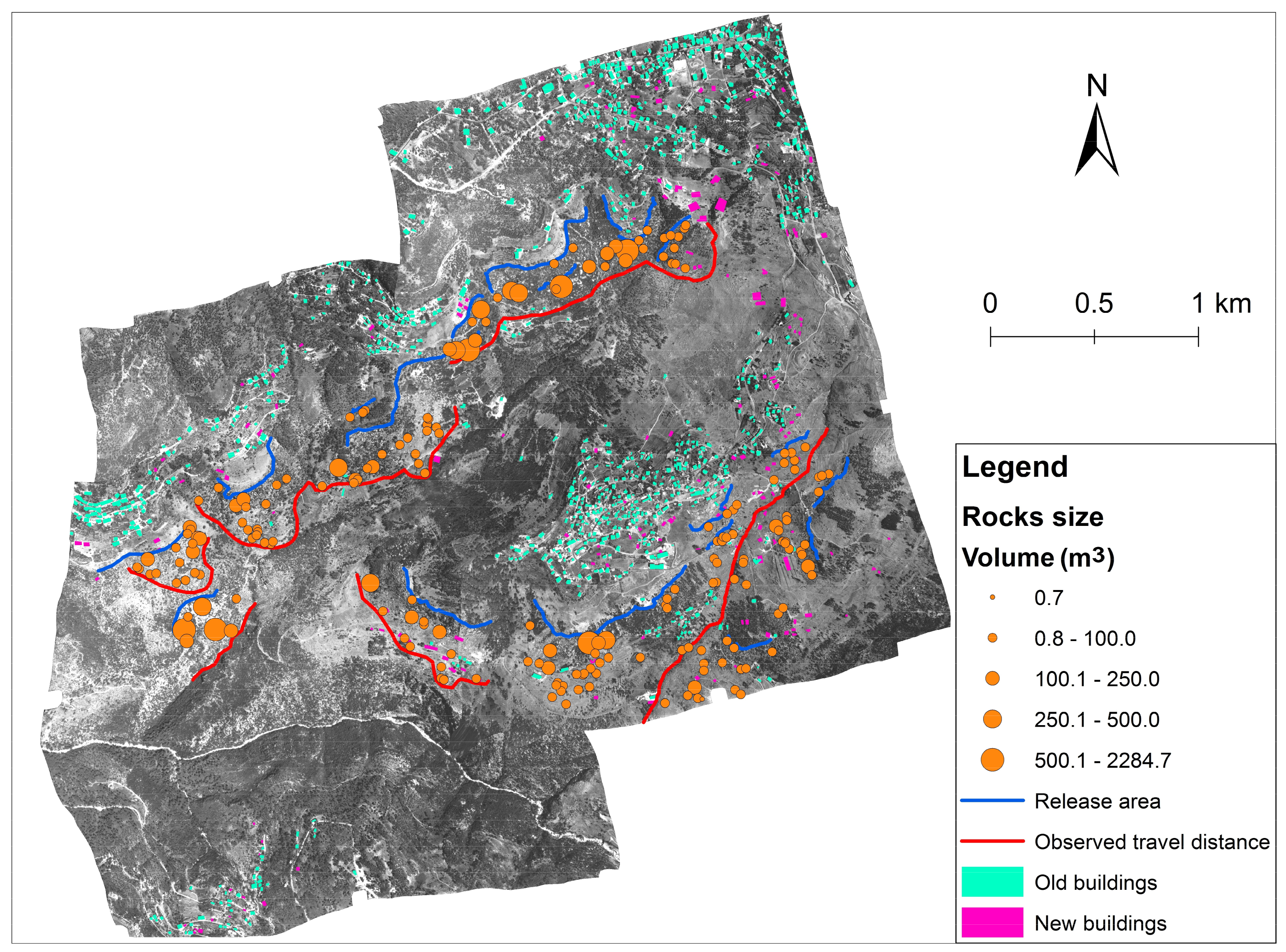
For instance, 209 deposited RFs (from previous RF events), of different rock sizes, were detected and mapped using the findings and information acquired throughout field trips (in June 2021) and aerial imaging [29]. The rock, already deposited from previous rockfall events, of sizes varying from 0.7 to 2284 cubic meters, were dispersed throughout the study area. The majority of the RFs had a volume of 25 cubic meters. Observations also revealed that certain built structures were in the trajectory of the potential falling rocks. These structures were built between the location of the RF source and their accumulation places.
The map (Figure 2) shows the locations of previous RFs, their rock volumes, and their maximal reaching distance (observed travel distance) as well as their release areas.
The maximum reaching points of RFs, represented by the lines in red in the map, varied in different areas because of the different characteristics of the landscape, such as the slope steepness, the rock type on the slope, and any obstacles that rocks may have encountered. In addition, all buildings that were observed in the orthophotos (existing before the year 2000) were digitized using the GEOAI Urban tool [30] and presented in the map. New buildings that were built during and after the year 2000 were digitized manually using the satellite basemap in ArcMap software (Version 10.8).

2.2. Runout Simulations

RF runout simulations are based on the shape; material properties; volume and density of the rocks; the slope angle and length (slope profile); the surface roughness of the slope, represented by the tangential coefficient of restitution; and the soil type, represented by normal coefficient of restitution [31,32]. The RF map, digital elevation model (with 5 meters spatial resolution and 10 meters vertical resolution), rock properties (rock density, block dimensions and shape), and the soil types and slope surface roughness, the first of which is directly related to normal (nCOR) and the latter of which is directly linked to the tangential (tCOR) coefficients of restitution, are inserted as inputs to run the RF runout simulations in Rockyfor3D software (Version 5.2.15) [33], a 3D modeling software for probabilistic and process-based simulations of RFs.
The mass of the RF blocks is calculated using the density and the volume of the rock at the source. The aerodynamic drag and rolling ability of the blocks are calculated based on their size and shape. The friction between each block and the slope is calculated using the roughness of the slope surface determined by the soil properties. The tangential coefficient of restitution measures rebound in a direction parallel to the contact surface, whereas the normal coefficient of restitution measures rebound perpendicular to the contact surface. These coefficients describe the ratio of rebound to incidence velocities during the collision.
The surface roughness is also determined by the heights of obstacles encountered, in a scattered pattern, along the slope. The heights are measured from the downward perspective of the slope [33]. The roughness in Rockyfor3D is represented by three classes: rg70, rg20, and rg10, which are used to calculate the tangential coefficient of restitution. These classes represent the probability of encountering different roughness levels, with rg70 being the most common (70% probability) and rg10 being the least common (10% probability). Each class is assigned to a roughness value, which represents the height of the obstacle that a falling rock would encounter. For example, if rg70 is equivalent to 0.05 meters, then 70% of the obstacles on the slope have a height of 5 centimeters. Two sets of simulations were conducted in Rockyfor3D. The first set simulated earthquake-triggered RFs, while the second set simulated RFs that occurred in fully moisture-saturated rocks and wet soils (representing the rainfall triggered RFs case). Among several output files generated by Rockyfor3D, only two outputs will be used in the analysis: (a) mean kinetic energy and (b) probability of reach. Using the said outputs of these simulations, the intersection impact points of the RF runout trajectories and the existing buildings prone to RF risks could be determined.
It is worth noting here that the directions by which rocks would fall from the source area to the accumulation zone were taken into consideration.
The following subsection describes the initial conditions (earthquake) that were used to simulate RFs in the software. The simulation parameters are derived from the collected data, such as the size and distribution of boulders observed in the aerial photos and during field visits, and these parameters are then calibrated to ensure that the simulated RFs match the real-world data as closely as possible.

2.2.1. Case of Earthquake

Three major faults in Lebanon (Yammouneh, Serghaya, and the Mount Lebanon thrust) are the most likely to generate earthquakes with magnitudes greater than 7. Additionally, secondary faults may cause earthquakes with magnitudes up to 6.5. Accordingly, Lebanon is at risk of experiencing moderate to severe earthquakes [34,35]. Harajli et al. 2002 [35] created a peak ground acceleration (PGA) map for Lebanon based on a 0.1 probability of exceedance in 50 years with an ultimate earthquake magnitude of 7. This map was used to calculate the initial velocity of RFs at the time of detachment, which is a parameter that is added to the simulation in the case of an earthquake. According to Harajli et al. (2002) [35] the local PGA is 0.20 m/s2 (g).
Mavrouli et al. (2009) [36] have indicated that the PGA along the slope is obtained by linear interpolation between the acceleration at the base (PGAb) and that at the slope crest (PGAcr). The authors have indicated that the acceleration at the base is 0.20 g and the acceleration at the crust is 1.5 × 0.20 = 0.3 g. Therefore, the value of the PGA for the slope face (PGAsf) is 0.27 g, which was interpolated using the values of the PGA at the base and crest and based on the average altitude of the study area (1100 m).
In other words, the PGA map was used to determine the initial velocity of RFs at the time of detachment in the event of an earthquake. The PGA along the slope (PGAsf) is 0.27 g, which was calculated using linear interpolation.
According to Saroglou et al. (2018) [37], the initial horizontal velocity of the block at the time of detachment could be determined by taking into consideration the equilibrium of the produced work and the kinetic energy, as indicated in the following equation:
V x = 2 × P G A s f × s
To start moving down the slope, the rock must be displaced by a small distance, denoted by Saroglou et al. (2018) [37], who set the value of s to 0.05 m in the calculations. Accordingly, the block’s initial horizontal velocity is 0.519 m/s, and its initial vertical velocity is considered to be negligible [37]. A value of 0.5 m was added to the initial height of the falling rock in the simulations, to account for the effect of the earthquake as Rockyfor3D software does not allow users to input the initial velocity or energy of a falling rock as a parameter. This value (0.5 m) is equivalent to the initial horizontal velocity of 0.519 m/s.

2.2.2. Case of Rainfall

The study area is characterized by a heavy rainfall pattern [38]. Most of the rocks in the area are karstified limestone, dolomitic limestone, and sandstone [39]. These rocks are porous and fractured, which allows water to easily seep into the pores and cracks. This increases the rock weight, the water pressure in the pores, and the width of the cracks during rainfall events. The wider the joints and fractures in a rock, the weaker it is [40]. In addition, water erodes the soil around rocks [41] and reduces the shear strength of soil materials [42]. Thus, rainfall is assumed to significantly increase the mass of a rock block without changing its volume, leading to an increase in the rock’s density. Heavy rainfall affects not only the rocks on a slope but also the materials that make up the slope itself. The high moisture content caused by heavy rainfall slows down rocks as they move down the slope [42]. In the simulations, the density of the rocks and soil was increased to account for the weight of the water they absorbed. The normal restitution coefficient, which represents rebound perpendicular to the contact surface when a rock bounces off the ground, was reduced to account for the damping effect of wet soil during impact [42].
The rainfall-triggered RF simulation was used to study how the moisture content of the soil and rocks affects the rebound velocity of rocks. The normal coefficient of restitution (nCOR) was lowered because the moisture content of the soil is inversely proportional to the coefficient of restitution. This means that the wetter the soil, the slower rocks will bounce off of it [42]. The coefficients of restitution are indicated in the following equations [43]:
nCOR = v r , n v i , n
tCOR = v r , t v i , t
where vi,n is the normal incident velocity, vi,t is the tangential incident velocity, vr,n is the normal rebound velocity and vr,t is the tangential rebound velocity.
Hence, in the simulation software, the original soil type value [39] was lowered to reduce the normal restitution coefficient, since Rockyfor3D software has seven standard soil types, each with a different normal restitution coefficient. The average density of the rocks was chosen based on their nature, with limestone having a density of 2550 Kg/m3 and sandstone having a density of 2350 Kg/m3. Nonetheless, the rocks in the simulation are assumed to be fully moisture saturated. To match the densities of fully moisture-saturated rocks [44], the densities of sandstone and limestone were increased from 2350 kg/m3 and 2550 kg/m3 to 2450 kg/m3 and 2650 kg/m3, respectively. The modeling parameters (rock density, boulder volume, boulder shape, surface roughness, digital elevation model) needed to run the simulations of 3D rockfall (RF) runout models in Rockyfor3D are included in each raster map in ESRI ASCII grid format. When creating the input data, the worst-case scenario was taken into account. This scenario considers the spherical shapes of rocks as well as the absence of forests/trees that could block the rock movement along the slope during RF.

2.2.3. Collection and Calculation Risk Equation Parameters

The annual cost of damage caused by RFs is referred to as RF risk. It is calculated by factoring in the likelihood of an RF (occurrence probability), the vulnerability of a structure to RF damage, and the economic value of the structure. The geology of the area, the slope angle, and the presence of fissures or other discontinuities in the rock all influence the possibility of an RF.
The vulnerability of a structure to RF damage is determined by its strength (to resist the RF impacting the structure), construction, and the materials employed in its construction.
The RF economic risk value, in the present study, is represented by the cost of repairing or replacing the damaged structure [10], without taking into account any human or any additional loss. Thus, the risk value of an RF, in a particular area, could be calculated by multiplying the said three factors using the following equation [22,24]:
R = M i P M i · P X J M i · P T X j · V i j · C
where R is the risk value resulting from rockfalls of magnitude Mi and intensity j on a vulnerable element positioned at a distance X from the RF source (the magnitude Mi is typically quantified by the volume of rock that falls), P(Mi) is the probability of rockfall occurrence of magnitude Mi, P(Xj|Mi) is the reach probability of a rockfall with intensity j reaching a spot at a distance X from the RF source (the intensity j is typically quantified by the kinetic energy created by the RF at a distance X from the RF source), P(T|Xj) is the probability of the element being at spatial point X at moment T of the rockfall, Vij is the element’s vulnerability to a rockfall of magnitude Mi and intensity j, and C is the value of the element at risk.

2.2.4. Probability of Occurrence—P(Mi)

According to Jaiswal and van Westen (2009) [45], the temporal probability is obtained by multiplying the annual exceedance probability (AEP) by the probability of landslide initiation, in the case of threshold exceedance. In this study, it is assumed that, whenever the threshold is exceeded, the RF is initiated, so the probability of landslide initiation is equal to one. It is worth noting that the threshold capable of inducing a rockfall is considered in this study to be equal to 5 according to the Richter scale in the case of earthquake, and to 100 mm cumulative precipitation in the case of rainfall over a period of 3 days.
The annual exceedance probability (AEP) is the chance that a general event of a certain magnitude/intensity/both will happen in any given year [24]. To determine the probability of RF, triggered by a factor whose intensity exceeds a certain threshold, within a certain time period, a Poisson probability model can be used [45,46,47]. The Poisson distribution model that can be used to calculate the probability of having a particular number of RFs in a time period t (N(t)) is given in the following:
P [ N ( t )     1 ] = 1 e t / µ
The mean recurrence interval between successive RFs (μ), can be obtained from the multi-temporal RF inventory data.
Case of earthquake:
Previous research has shown that only earthquakes with a magnitude of 5 or greater can trigger slope failures [48,49], as strong ground motions have been known to trigger RFs in the past [50].
As large magnitude earthquakes (magnitude above 5 according to the Richter scale) have occurred in previous centuries in Lebanon, Brax et al. 2019 [51] assessed the published studies on earthquakes in Lebanon and compiled a list of events with estimated micro-seismic epicenters. This list includes the earthquakes that occurred in the years 551 (with magnitude 7.3), 1170 (magnitude 7.3), 1202 (magnitude 7.6), the two earthquakes in the year 1759 (on 30 October with magnitude 6.6 and on 25 November with magnitude 7.4) and lastly the earthquake of the year 1837 (magnitude 7.0) [52].
The return period of large earthquakes hazards in Lebanon is estimated to be 475 years [52,53]. In the present study, the return period is considered the same (475 years) according to aforementioned references. According to Equation (6), and during the time period (t) of 1 year, the temporal probability (annual probability) is equal to 0.002.
Case of heavy rainfall:
Intense rainfall can alter hydrogeological conditions and water levels, triggering surface movements of soils and altering materials. These movements can initiate RFs, landslides or debris flows. Knowing that there is a direct relationship between the amount of accumulated rainfall and the occurrence of instabilities, one can say that, generally, the greatest probability of these instability events occurs during the periods of heavy precipitations [54].
A recent study conducted by Leyva et al. (2022) [54] has investigated the relationship between rainfall and RFs over the period 2010–2016 in the Anaga Nature Reserve, a mountainous region with steep slopes in Tenerife. The cumulative rainfall over a period of 3 days was the amount of rainfall considered in this study.
The results show that (a) there is a strong correlation between rainfall and RFs, as the probability of an RF occurrence increases significantly after periods of heavy rainfall, and that (b) the amount of rainfall required to trigger an RF varies depending on the slope angle. In the latter context, the authors found that, on slopes with an angle of 45 degrees, the amount of rainfall required to trigger an RF is about 100 mm over a period of 3 days, as well as 200 mm accumulated rainfall for slope angle of 60 degrees.
With respect to the amount rainfall that could initiate slope instability, the present study uses the same method adopted by the aforementioned research [54], which considered the cumulative rainfall amount over a 3-day period.
Further, and to be more conservative while forecasting the slope instability risks, the worst-case scenario, which considers the least amount of rainfall (100 mm) corresponding to the shallowest slope angle (45 degrees), was taken into account in the present study.
In the present article, daily precipitation data recorded from the year 1981 through to the present (2023) was obtained from the Earthdata webpage of NASA [55]. By analyzing the obtained data, the cumulative heavy rainfall (≥100 mm) over three consecutive days was detected in the years 2010 and 2019, in the months of December and January respectively. Thus, in the present research, the return period for rainfall-triggered RFs is assumed to be 9 years, while, according to Equation (6), which considers t = 1, the annual probability of RF occurrence is calculated and is then equal to 0.105.

2.2.5. Reach Probability—P (Xj|Mi)

Reach probability is the percentage of blocks that reach a distance from the RF source cliff. A simple calculation can be conducted by dividing the number of blocks that passed through a given distance by the total number of falling blocks [56]. This is typically used to determine the RF runout zone, which represents the area where blocks are likely to stabilize after they have fallen from the cliff. For this probability, Rockyfor3D calculates the reach probability in each location of the zone of interest.
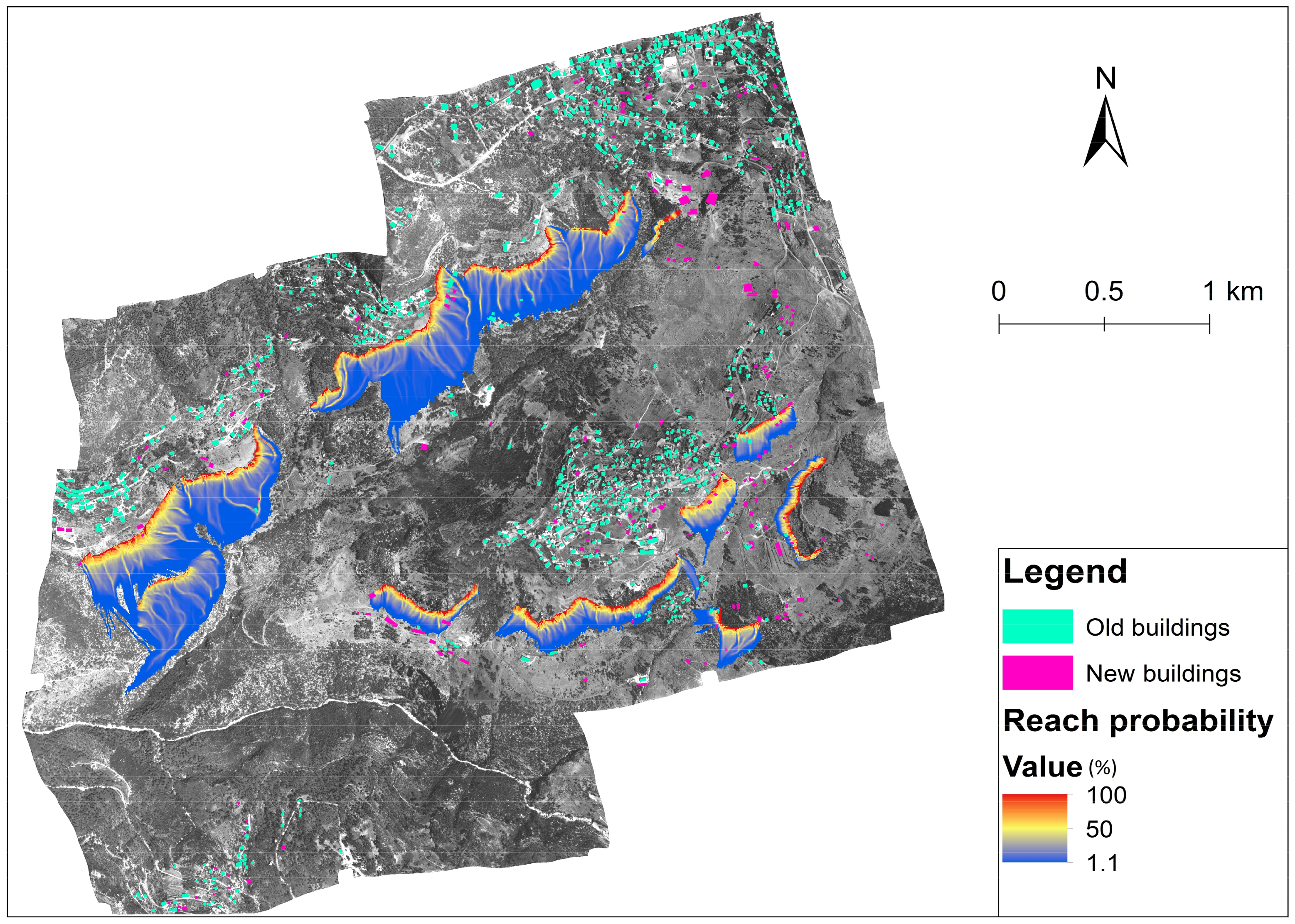
The reach probabilities are then calculated for each scenario, i.e., of earthquake and rainfall cases as presented in Figure 3 and Figure 4, respectively. Finally, intersection points are created between the runout zones of simulated RFs and the existing buildings already rasterized. Accordingly, the reach probabilities are attributed to these points.

2.2.6. Probability of the Element Being at Point X at the Time of the Rockfall Occurrence P (T|Xj)

The spatial probability of the element being at point X at time T of the rockfall occurrence is assumed to be equal to the point of intersection created between simulated RFs and buildings. This is due to the fact that buildings (containing the intersection points) are fixed in position and are located on the trajectory or fallen rocks.

2.2.7. Physical Vulnerability—(Vij)

In the context of RF hazards, many authors have defined two types of corresponding vulnerabilities: societal vulnerability [57] and physical vulnerability [58]. The first of these is related generally to human injuries and deaths that are the result of RF events.
RF physical vulnerability is the degree to which a set of assets can be damaged or lost due to RFs [59]. Both types of vulnerability represent a key factor in RF risk assessment and management, as their estimation is essential for making reliable predictions and mitigation plans for RF impacts. Nonetheless, the present study is limited to an examination of RF risk from a physical vulnerability perspective.
According to UNDP/UNESCO 1982 [60], four main groups of methods exist for assessing the level of vulnerability of a structure: (i) categorization methods, (ii) inspection and empirical (rating) methods, (iii) analytical methods, and (iv) experimental methods.
The categorization methods classify structures into typological classes based on their structural type, construction materials, and construction techniques. They are employed because different structural typologies have different vulnerabilities to natural hazards.
The inspection and empirical (rating) methods assign numerical values to each structure based on its condition. Generally, this is done by inspecting the structure and looking for signs of damage, such as cracks, deterioration, and poor construction practices.
The analytical methods calculate the resistance of a structure against natural hazards damage by using civil engineering equations and computer models.
The experimental methods involve testing the structural components and entire structures to determine their properties. This type of vulnerability assessment for structures is considered the most accurate; however, it is also the most expensive and time-consuming method.
In the present study, a combination of the first three of these four methods is applied. Accordingly, the vulnerability was assessed using the combined methodology developed by Li et al. (2010) [61], and was calculated according to the following:
V = f I , R = 2 ( I R ) 2   if   I R 0.5 1 2 ( 1 I R ) 2   if   0.5 < I R 1.0 1.0   if   I R > 1.0
where V represents the vulnerability, I represents the RF intensity, and R represents the resistance of buildings.
The RF intensity I in this study is scaled from 0 to 1, based on the previous research by Lateltin et al. (2005) [62]. The authors indicated that I is determined mainly by the RF kinetic energy and that, therefore, the intensity of RFs can be estimated according to Table 1.
The resistance of buildings, R, is calculated as the following equation using resistance factors associated with the following four variables: structure typology (ε1), state of maintenance (ε2), construction quality (ε3) and number of floors (ε4) as determined by Li et al. (2010) [61].
R = ( ε 1 × ε 2 × ε 3 × ε 4 ) 1 / 4
With respect the first variable, buildings must be categorized into different structural typologies where each topology has a specific resistance factor ( ε 1). The resistance factors for the three structural typologies are defined as follows: brick masonry ( ε 1 = 0.3), stone masonry ( ε 1 = 0.6), and reinforced concrete ( ε 1 = 1).
Once the buildings have been categorized, they must be inspected and assigned numerical values according to rating (empirical) methods in order to represent the state of maintenance ( ε 2). This involves rating the structure by looking for signs of damage and poor construction practices, as follows: damaged ( ε 2 = 0.2), distressed ( ε 2 = 0.4), good ( ε 2 = 0.8), and excellent ( ε 2 = 1).
Furthermore, the construction quality evaluation is determined by several factors, such as the type of construction, the materials used, and the age of the structure. The higher the quality, the higher the resistance and the lower the vulnerability rating. The resistance values corresponding to the quality are defined as follows: low ( ε 3 = 0.2), moderate ( ε 3 = 0.5), and high ( ε 3 = 1).
The fourth resistance factor corresponds with the number of floors, where the higher the building, the lower the vulnerability rating. This assumption, made by Singh et al. (2021) [8], is based on the fact that taller buildings typically have more depth and solid foundations as well as core walls and shear walls. These resistance factors are defined as follows: 1 floor ( ε 4 = 0.2), 2 floors ( ε 4 = 0.5), 3 and more floors ( ε 4 = 1).
Consequently, the most critical parameters to be determined are I and R. The first parameter, I, was obtained through the simulation results for each scenario. By examining the simulation output, specifically the mean kinetic energy map, the kinetic energy value was extracted from the raster map at the point where the rockfall impacts the side of the building. This point represents the potential impact site on the building structure.
The coefficient R was calculated using Equation (7), wherein distinct values were assigned to each parameter (ε1, ε2, ε3, and ε4) in the equation for every building. These assignments were based on the assessment of the buildings’ characteristics and conditions situated along the trajectory of rockfall propagation.

2.2.8. Value of the Element at Risk

The cost of repairing building damage caused by RFs is difficult to estimate because it depends on many factors, such as the severity of the damage, the type of building, and the cost of materials and labor. Additionally, the cost of repairing damage can vary significantly depending on the location of the building. For example, it may be more expensive to repair building damage in a peripheral area than in a more centrally urbanized area. The area of a building that is exposed to RFs could be employed to accurately measure the value of the element at risk [63]. Considering the area of buildings that are exposed to RF risk leads to a better understanding of the potential damage caused by the RFs. Based on expert opinion and according to experience in assessing building damages [64], the cost of damage is estimated, in this study, to be 400 USD per square meter. This cost is expensive considering that the zone of interest is a peripheral area and requires additional cost to transport materials.

3. Results and Discussion

Recalling the previous section, 1000 simulations for each scenario (earthquake and rainfall scenarios), were performed. An additional value of the horizontal kinetic energy was added to represent the effect of earthquakes on rock blocks in the release area. This is expressed by lifting up each block by 0.5 m, as suggested in Section 2.2.1. However, in the case of the rainfall scenario, two simulation parameters were changed differently. The change of the first is represented by lowering the normal coefficient of restitution (soil type), which leads to a damping effect on the rock block while moving down along the slope. The second parameter is the density of rock block itself, and this is increased due to water absorption during or right after a rainfall period. The change in the second parameter leads to an increase of moisture content and therefore an increase of the density of rock block. The densities of sandstone and limestone were increased from 2350 kg/m3 and 2550 kg/m3 to 2450 kg/m3 and 2650 kg/m3 (see Section 2.2.2).
The results reveal that 48 buildings in the study area could potentially be hit by RFs in both the earthquake and rainfall scenarios. However, in the earthquake scenario, an additional 5 buildings could potentially be hit, for a total 53 damaged buildings. This suggests that earthquakes can dislodge more rocks and cause them to fall over a wider area.
Regarding the damage size, the study also shows that earthquakes will potentially present more damage to buildings in the RF impact area than in the case of rainfall-triggered RF. Findings show that the risk of damage to the majority of buildings was higher in the earthquake scenario compared with the rainfall scenario. This is likely because the earthquake vibrations can tremble buildings and make them more vulnerable to damage from falling rocks. This is also related to the observation that the highest impact energy resulting from the case of earthquake was 10,673.7 KJ, while, for that of rainfall, it was 10,451 KJ.
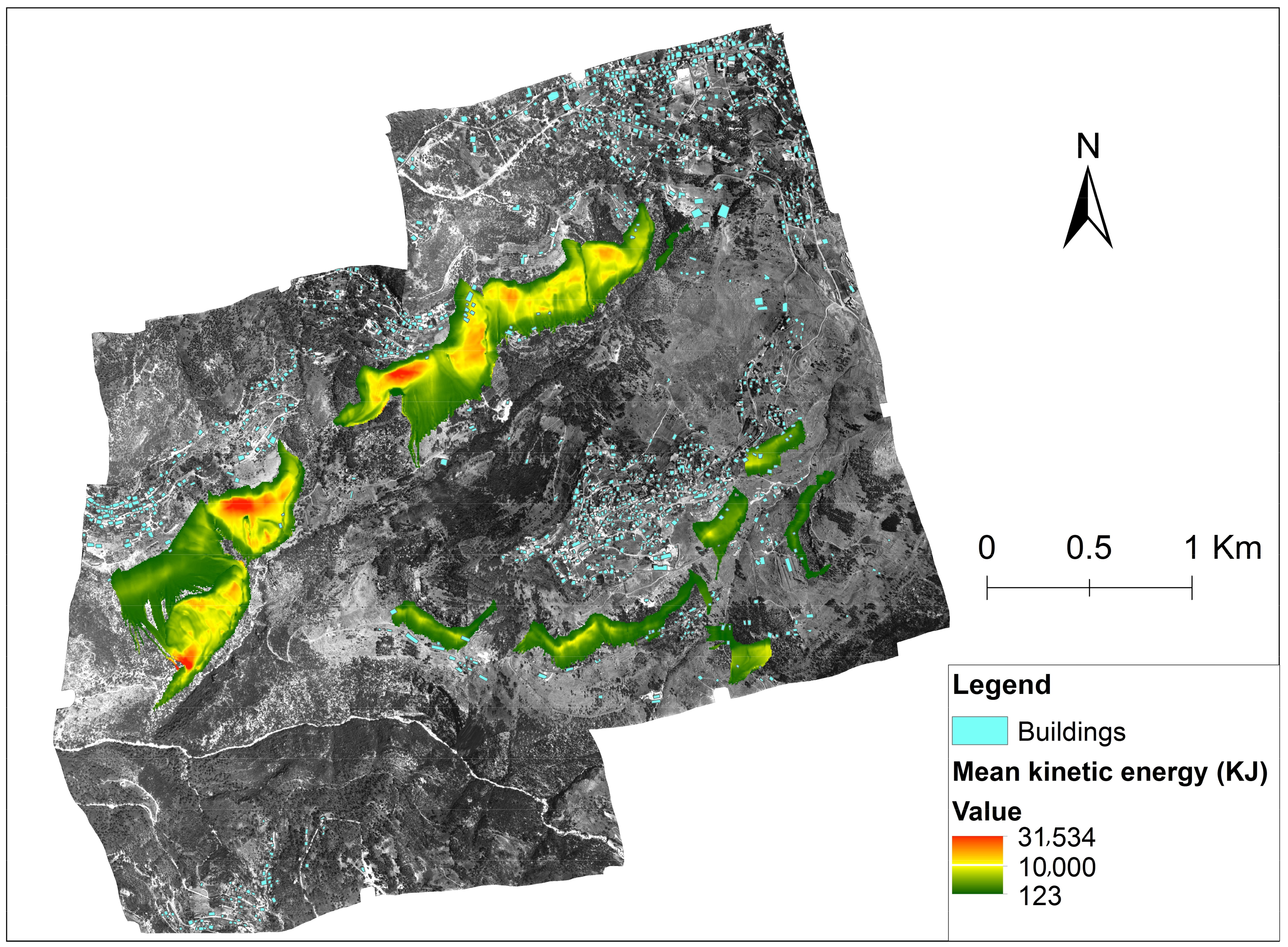
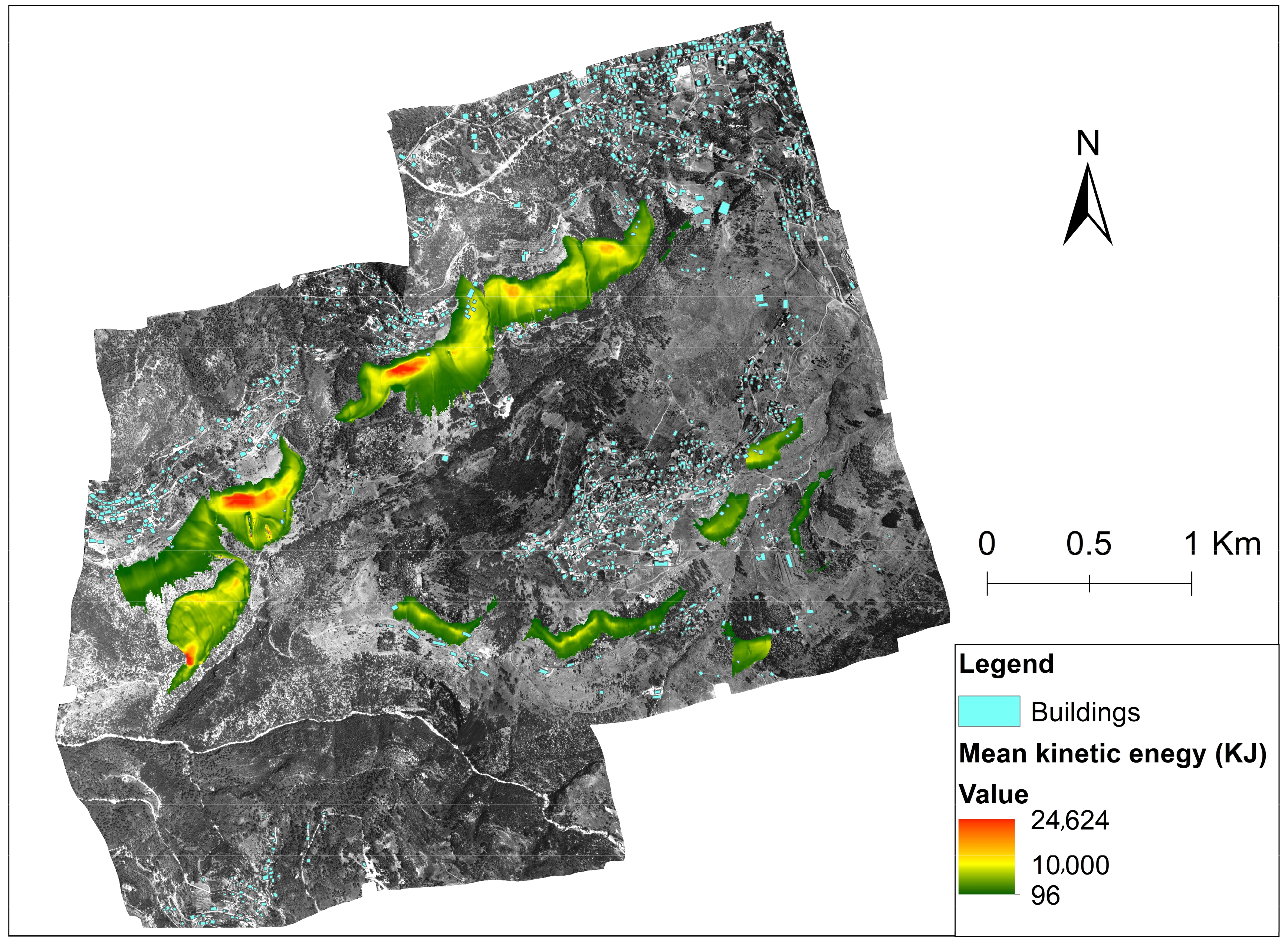
The mean kinetic energies for RFs in both scenarios are presented in Figure 5 and Figure 6. It is worth noting that the potential highest kinetic energies in both scenarios are observed in the same spots, and that this is due to the steepness of slope, which is is around 60 to 65 degrees. Additionally, and with respect to building conditions that affect their vulnerability, the field survey of buildings that could potentially be hit by RFs has revealed that 85% of the buildings are made of concrete, 11% made of stone masonry and 4% made of brick masonry. In addition, 53% of these buildings are well-maintained and in excellent condition, 32% are in good condition and 15% are in damaged/distressed condition. Notably, nearly one-third (28%) of the buildings are poorly constructed.
Regarding vulnerabilities, the calculation results are equal to 1 for all of the buildings except for one of them (0.68 for earthquake and 0.62 in rainfall case), this is explained by (1) the high intensity of RFs, as mean kinetic energy was higher than 300 KJ, and (2) the low resistance of buildings against RF impact.
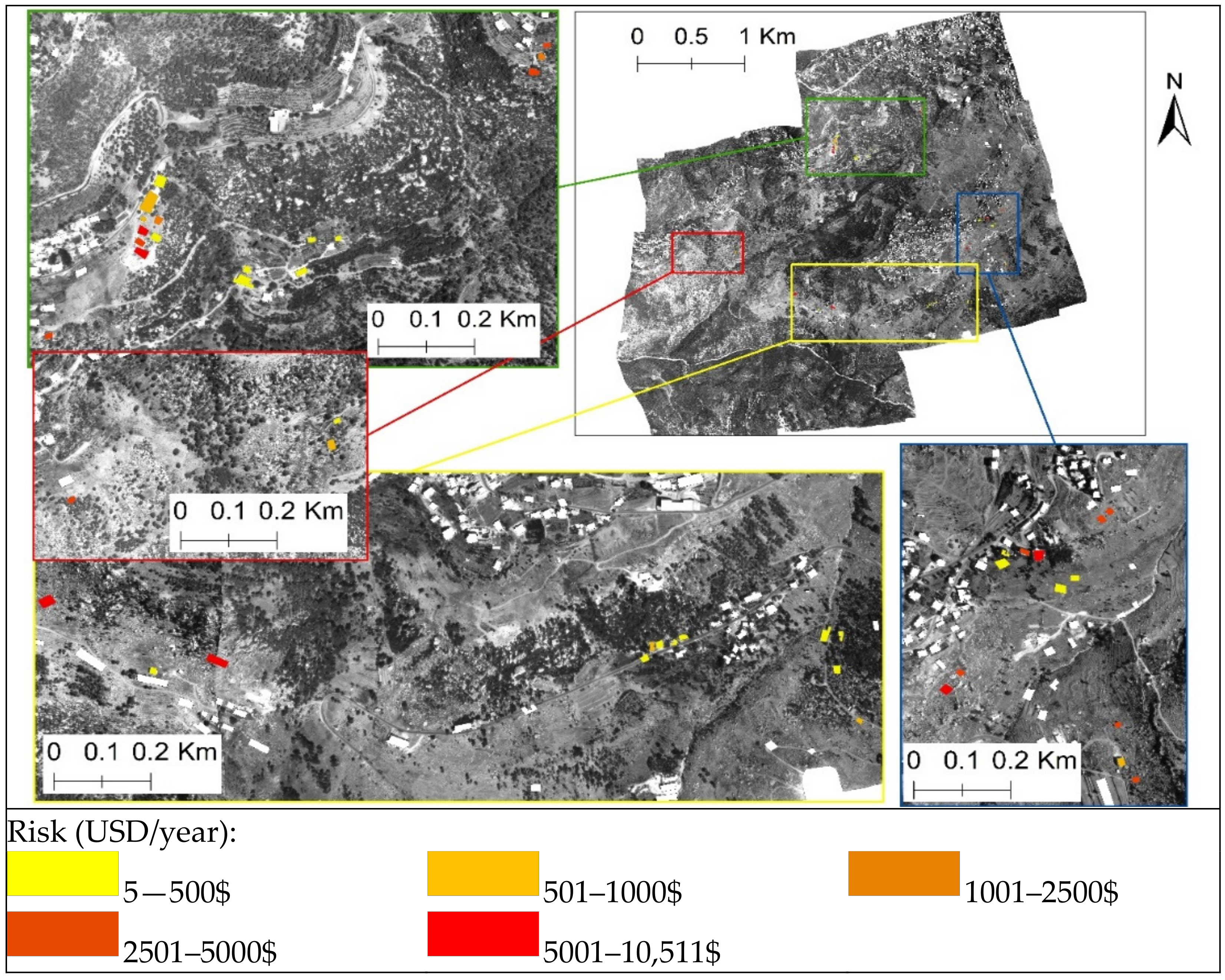
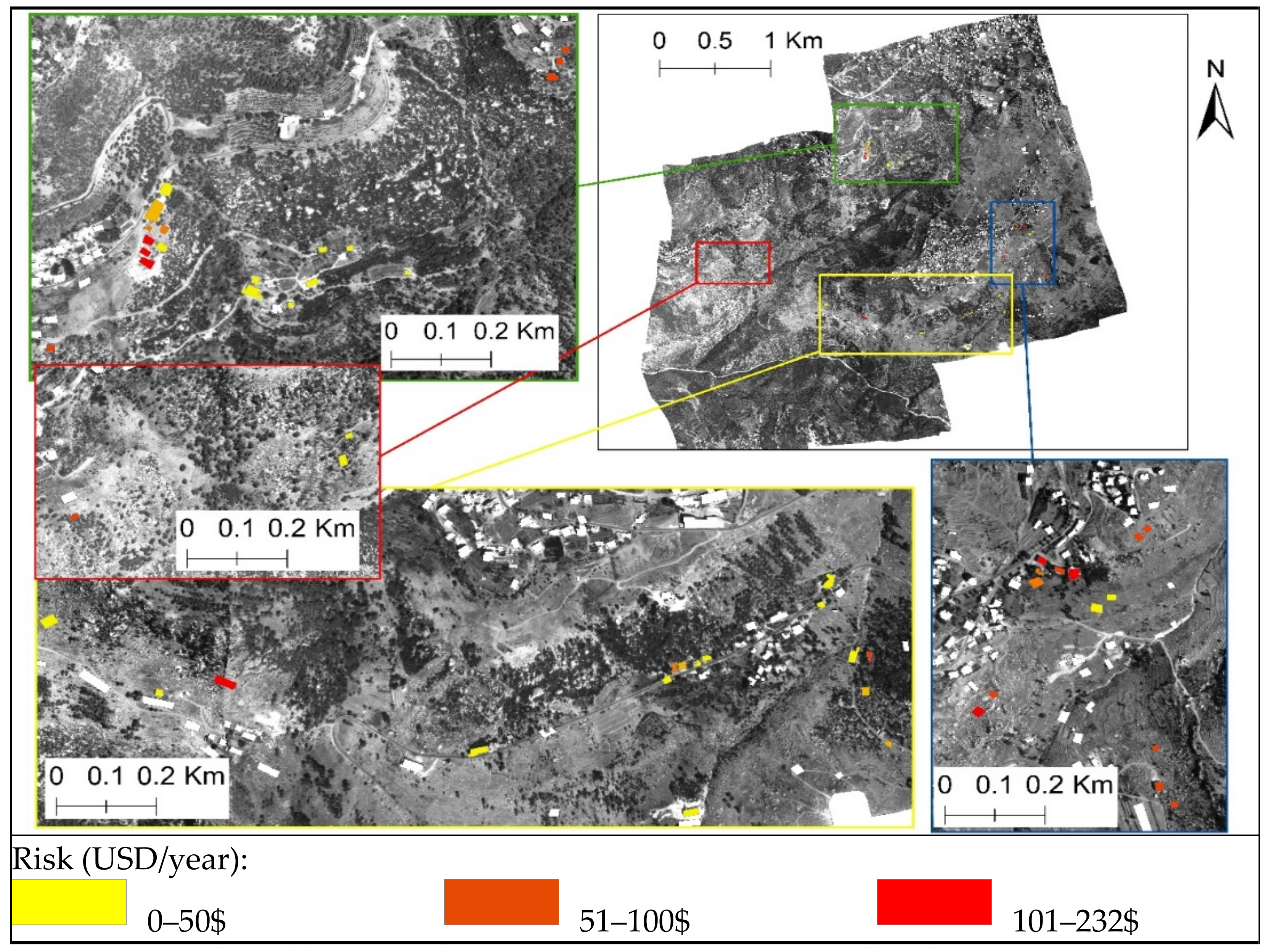
These results are combined with the impact probability and the value of elements at risk according to equation 5, allowing one to compute the annual cost of RF risk on buildings (as shown in Figure 7 and Figure 8). Results show that the highest cost of RF risk is of 232 USD in case of earthquake, and 10,511 USD in the case of rainfall, per annum.
The proposed approach for risk assessment (quantitative method) in this study, is limited by the absence of statistically representative historical catalogues of RF events as well as their impacts and damages in Lebanon. This makes it difficult to accurately characterize the frequency distribution of RF volumes for individual sites, which is essential for using the approach in practice.
The observed size of deposited rockfalls varies significantly, ranging from 0.7 to 2284 cubic meters. However, for the purpose of this study, a volume of 25 cubic meters was selected as the initial estimate for the volume of the rockfalls that originated from the release areas. This choice was based on the high frequency of this size within the study area, without taking into consideration the fragmentation. Given the broad spectrum of sizes observed, it was assumed that this volume could be the better representative of typical rockfalls from release areas. Larger rockfalls are expected to yield increased runout distances and higher kinetic energies on the slope, while smaller rockfalls are anticipated to have shorter runout distances and lower kinetic energies.
Risk assessments are also affected by the quality of the database that is used to calculate the vulnerability functions. Additionally, the data needed to fully quantify the value of elements at risk (e.g., buildings, infrastructure) is not always available. This introduces further uncertainty into the estimated costs.
Despite these limitations with respect to RF events, dating the RFs can improve the estimated return periods, as it can provide information on how many boulders of a given size could potentially fall in a specific time period.
The locations where RFs commence (release areas) are difficult to detect and to correctly map. Nonetheless, with the help of aerial photographs and field investigation, the release zones on the unstable slope were located and mapped.
Additionally, partially detached rock blocks and rock masses overlying joints, which are orientated in a way that makes them more likely to break, are indicators of possible RF release zones. Finally, the simulations were carried out where boundaries of the release areas were chosen, in order to cover the locations of all unstable blocks on hills.

4. Concluding Remarks and Future Research

Although no historical information on RFs is available, the presented case study demonstrates that advanced numerical modelling techniques can be used to establish a valuable RF risk evaluation method that can be implemented to improve the quantitative risk assessment at various levels of complexity based on the available data. The simulation was validated by comparing the results of each simulation to the actual observed rockfall deposits. It was noted that the locations of the deposited rockfalls in the simulation aligned with the actual deposition sites.
This study developed a new methodology with which to calculate the risk of RFs for individual buildings in a rural area. The study first used a computer model to simulate, using a computational approach, the RF runout zone and other characteristics, such as the speed, energy and reach probability of the RFs. Then, the study considered both the intensity of the RFs and the resistance of the buildings to calculate the vulnerability of each building. The resistance of each building encompasses factors such as the construction structure, number of floors, building type, and maintenance state. Moreover, the economic impacts of RF events are estimated. Finally, the study created a risk map for the study area by combining the risk maps for different buildings.
The proposed risk analysis method for RFs has several advantages over existing methods. First, it is particularly well-suited for risk problems that are spread out over a large area. Second, it can combine all stages of risk assessment into one process, which can make the assessment more efficient and precise. Third, it decreases the number of assumptions that need to be made about the physical components of risk, such as the hazard, probability, and energy of impacts on structures.
However, there are still some concerns about the method because there is a lack of statistically reliable data on both RF events, damage, and cost of assets. This lack of data can make it difficult to validate the results of the risk assessment. Nevertheless, the proposed method provides a good estimate of risk, which is essential for evaluating the effectiveness of RF mitigation measures.
Generally, the proposed risk analysis method is a promising new approach for assessing the risk of RFs, as it is more comprehensive and accurate than existing methods. However, that method is still under development, requiring more data to validate the results. Nevertheless, and despite some limitations in the risk assessment, the risk map can still be used to identify areas at high risk of RFs and to develop mitigation measures. Mitigation measures can reduce the hazard or susceptibility of the community to RFs, and they are especially important in high-risk areas. Given the high number of inhabitants in this study area, upcoming studies are needed to carry out an assessment of the RF risk on human lives.
The application of quantitative risk assessment methods is not limited to rockfalls, it can also be applied to other types of landslides. Identifying hazards, assessing the probability of occurrence, and estimating the potential impact are necessary across different types of landslides. However, specific models and techniques may need to be adapted or developed based on the unique characteristics of each landslide type. It is essential to emphasize the modern significance of machine learning algorithms, which have enormous potential in advancing the study of rockfalls and can be fundamental in further research. For instance, the study by Rafiei Sardooi et al. (2021) [65] on landslide risk assessment provides a good example of this potential. Their methodology not only offers a framework for assessing the risk of various landslide types but also delivers remarkably valuable results. Machine learning (ML) and artificial intelligence (AI) can significantly contribute to quantifying risk in several ways, such as automated geological feature mapping and landslide simulations, etc. AI can integrate all of the information and data into a single interface in order to analyze landslide risks and develop risk maps using various models and methods like the finite element method (FEM), limit equilibrium method (LEM), and quantitative risk assessment (QRA).
Moreover, the integration of both physical and social science aspects in comprehending and evaluating landslide mitigation measures by community perception represents a groundbreaking approach. This entire perspective not only raises innovation but also raises public trust in the efficacy of such measures [66].

Author Contributions

Conceptualization, M.A.-S. and J.A.-G.; methodology, M.A.-S., J.A.-G. and W.A.-S.; software, M.A.-S. and G.F.; validation, M.A.-S., W.A.-S., J.A.-G., G.F. and P.-C.G.; formal analysis, M.A.-S. and W.A.-S.; investigation, M.A.-S.; resources, J.A.-G. and P.-C.G.; data curation, M.A.-S.; writing—original draft preparation, M.A.-S.; writing—review and editing, M.A.-S., W.A.-S., J.A.-G., G.F. and P.-C.G.; visualization, M.A.-S. and W.A.-S.; supervision, J.A.-G.; project administration, J.A.-G. and P.-C.G. All authors have read and agreed to the published version of the manuscript.

Funding

This research received no external funding.

Institutional Review Board Statement

Not applicable.

Informed Consent Statement

Not applicable.

Data Availability Statement

The data presented in this study are available on request from the corresponding authors.

Conflicts of Interest

The authors declare no conflict of interest.

References

  1. Mourey, J.; Lacroix, P.; Duvillard, P.-A.; Marsy, G.; Marcer, M.; Ravanel, L.; Malet, E. Rockfall and Vulnerability of Mountaineers on the West Face of the Aiguille du Goûter (Classic Route up Mont Blanc, France), an Interdisciplinary Study. Nat. Hazards Earth Syst. Sci. 2021, 1–29. [Google Scholar] [CrossRef]
  2. Zheng, L.; Wu, Y.; Zhu, Z.; Ren, K.; Wei, Q.; Wu, W.; Zhang, H. Investigating the Role of Earthquakes on the Stability of Dangerous Rock Masses and Rockfall Dynamics. Front. Earth Sci. 2022, 9, 1338. [Google Scholar] [CrossRef]
  3. Guzzetti, F. Rockfall BT—Encyclopedia of Natural Hazards; Bobrowsky, P.T., Ed.; Springer: Dordrecht, The Netherlands, 2013; pp. 875–877. ISBN 978-1-4020-4399-4. [Google Scholar]
  4. Scavia, C.; Barbero, M.; Castelli, M.; Marchelli, M.; Peila, D.; Torsello, G.; Vallero, G. Evaluating rockfall risk: Some critical aspects. Geosciences 2020, 10, 98. [Google Scholar] [CrossRef]
  5. Briones-Bitar, J.; Carrión-Mero, P.; Montalván-Burbano, N.; Morante-Carballo, F. Rockfall research: A bibliometric analysis and future trends. Geosciences 2020, 10, 403. [Google Scholar] [CrossRef]
  6. Hantz, D.; Corominas, J.; Crosta, G.B.; Jaboyedoff, M. Definitions and concepts for quantitative rockfall hazard and risk analysis. Geosciences 2021, 11, 158. [Google Scholar] [CrossRef]
  7. Crosta, G.; Agliardi, F.; Frattini, P.; Lari, S. Key Issues in Rock Fall Modeling, Hazard and Risk Assessment for Rockfall Protection. In Engineering Geology for Society and Territory; Springer: Berlin/Heidelberg, Germany, 2015; pp. 43–58. ISBN 978-3-319-09056-6. [Google Scholar]
  8. Singh, A.; Kanungo, D.; Singh, P. Site-Specific Risk Assessment of Buildings Exposed to Rock Fall in India—A Case Study. In Understanding and Reducing Landslide Disaster Risk; Springer: Berlin/Heidelberg, Germany, 2021; pp. 475–482. ISBN 978-3-030-60226-0. [Google Scholar]
  9. Mavrouli, O.; Corominas, J. Rockfall vulnerability assessment for reinforced concrete buildings. Nat. Hazards Earth Syst. Sci. 2010, 10, 2055–2066. [Google Scholar] [CrossRef]
  10. Lollino, G.; Giordan, D.; Crosta, G.B.; Corominas, J.; Azzam, R.; Wasowski, J.; Sciarra, N. Engineering Geology for Society and Territory—Volume 2: Landslide Processes; Springer: Berlin/Heidelberg, Germany, 2015; Volume 2, ISBN 9783319090573. [Google Scholar]
  11. Žabota, B.; Kobal, M. A new methodology for mapping past rockfall events: From mobile crowdsourcing to rockfall simulation validation. ISPRS Int. J. Geo-Information 2020, 9, 514. [Google Scholar] [CrossRef]
  12. Romeo, S.; Cosentino, A.; Giani, F.; Mastrantoni, G.; Mazzanti, P. Combining ground based remote sensing tools for rockfalls assessment and monitoring: The poggio baldi landslide natural laboratory. Sensors 2021, 21, 2632. [Google Scholar] [CrossRef]
  13. Corominas, J.; Mavrouli, O.; Ruiz-Carulla, R. Rockfall Occurrence and Fragmentation BT—Advancing Culture of Living with Landslides; Sassa, K., Mikoš, M., Yin, Y., Eds.; Springer: Cham, Switzerland, 2017; pp. 75–97. [Google Scholar]
  14. Bertolo, D. A decision support system (DSS) for critical landslides and rockfalls and its application to some cases in the Western Italian Alps. Nat. Hazards Earth Syst. Sci. 2017, 1–31. Available online: https://nhess.copernicus.org/preprints/nhess-2017-396/ (accessed on 3 March 2024).
  15. Farvacque, M.; Lopez-Saez, J.; Corona, C.; Toe, D.; Bourrier, F.; Eckert, N. Quantitative risk assessment in a rockfall-prone area: The case study of the Crolles municipality (Massif de la Chartreuse, French Alps). Geomorphol. Reli. Process. Environ. 2019, 25, 7–19. [Google Scholar] [CrossRef]
  16. Wang, X.; Frattini, P.; Crosta, G.B.; Zhang, L.; Agliardi, F.; Lari, S.; Yang, Z. Uncertainty assessment in quantitative rockfall risk assessment. Landslides 2014, 11, 711–722. [Google Scholar] [CrossRef]
  17. Mavrouli, O.C.; Abbruzzese, J.; Corominas, J.; Labiouse, V. Review and advances in methodologies for rockfall hazard and risk assessment. Adv. Nat. Technol. Hazards Res. 2014, 34, 179–199. [Google Scholar] [CrossRef] [PubMed]
  18. Corominas, J.; Mavrouli, O.C. Quantitative Risk Assessmenent for Buildings due to Rock-Falls: Some Achievements and Challenges. 2011. Available online: https://api.semanticscholar.org/CorpusID:819582 (accessed on 3 March 2024).
  19. Ferrari, F.; Giacomini, A.; Thoeni, K. Qualitative Rockfall Hazard Assessment: A Comprehensive Review of Current Practices. Rock Mech. Rock Eng. 2016, 49, 2865–2922. [Google Scholar] [CrossRef]
  20. Agliardi, F.; Crosta, G.B.; Frattini, P. Integrating rockfall risk assessment and countermeasure design by 3D modelling techniques. Nat. Hazards Earth Syst. Sci. 2009, 9, 1059–1073. [Google Scholar] [CrossRef]
  21. Baecher, G.; Christian, J. Reliability and Statistics in Geotechnical Engineering; John Wiley & Sons: Hoboken, NJ, USA, 2003. [Google Scholar]
  22. Corominas, J.; Westen, C.J.; Frattini, P.; Cascini, L.; Malet, J.-P.; Fotopoulou, S.; Catani, F.; Eeckhaut, M.; Mavrouli, O.; Agliardi, F.; et al. Recommendations for the quantitative analysis of landslide risk. Bull. Eng. Geol. Environ. 2014, 73, 209–263. [Google Scholar] [CrossRef]
  23. Corominas, J.; Copons, R.; Moya, J.; Vilaplana, J.M.; Altimir, J.; Amigó, J. Quantitative assessment of the residual risk in a rockfall protected area. Landslides 2005, 2, 343–357. [Google Scholar] [CrossRef]
  24. Fell, R.; Ho, K.; Lacasse, S.; Leroi, E. A Framework for Landslide Risk Assessment and Management; CRC Press: Boca Raton, FL, USA, 2005. [Google Scholar]
  25. Moos, C.; Fehlmann, M.; Trappmann, D.; Stoffel, M.; Dorren, L. Integrating the mitigating effect of forests into quantitative rockfall risk analysis—Two case studies in Switzerland. Int. J. Disaster Risk Reduct. 2018, 32, 55–74. [Google Scholar] [CrossRef]
  26. Corominas, J.; Mavrouli, O. Rockfall Quantitative Risk Assessment. In Rockfall Engineering; Wiley: Hoboken, NJ, USA, 2013; pp. 255–301. ISBN 9781118601532. [Google Scholar]
  27. Dussauge-Peisser, C.; Helmstetter, A.; Grasso, J.R.; Hantz, D.; Desvarreux, P.; Jeannin, M.; Giraud, A. Probabilistic approach to rock fall hazard assessment: Potential of historical data analysis. Nat. Hazards Earth Syst. Sci. 2002, 2, 15–26. [Google Scholar] [CrossRef]
  28. Dubertert, L. Geological Maps of Syria and Lebanon at 1.50.000; No. 21 Sheets with Explicative Note; Minister of Public Affairs: Beiru, Lebanon, 1953.
  29. Al-Shaar, M.; Gérard, P.-C.; Faour, G.; Al-Shaar, W.; Adjizian-Gérard, J. Comparison of Earthquake and Moisture Effects on Rockfall-Runouts Using 3D Models and Orthorectified Aerial Photos. Geographies 2023, 3, 110–129. [Google Scholar] [CrossRef]
  30. Nasrallah, H.; Shukor, M.; Ghandour, A.J. Sci-Net: Scale-invariant model for buildings segmentation from aerial imagery. Signal Image Video Process 2023, 17, 2999–3007. [Google Scholar] [CrossRef]
  31. Khatiwada, D.; Dahal, R.K. Rockfall hazard in the Imja Glacial Lake, eastern Nepal. Geoenviron. Disasters 2020, 7, 29. [Google Scholar] [CrossRef]
  32. Jones, C.L.; Higgins, J.D.; Andrew, R.D. Colorado Rockfall Simulation Program Version 4.0 Manual. In Colorado Department of Transportation, Denver, CO; Institute of Agricultural Economics: Belgrade, Serbia, 2000; p. 80222. ISBN 3037579749. [Google Scholar]
  33. Luuk Dorren, A.K. Rockyfor3D (v5.2) Revealed—Transparent Description of the Complete 3D Rockfall Model. ecorisQ Pap. 2015, 1–37. Available online: https://www.ecorisq.org/docs/Rockyfor3D_v5_2_EN.pdf (accessed on 25 September 2022).
  34. Elias, A.R. Short Notice on Earthquake Hazard in Lebanon; Geology Department, American University of Beirut: Beirut, Lebanon, 2012; pp. 1–4. [Google Scholar]
  35. Harajli, M.; Sadek, S.; Asbahan, R. Evaluation of the seismic hazard of Lebanon. J. Seismol. 2002, 6, 257–277. [Google Scholar] [CrossRef]
  36. Mavrouli, O.; Corominas, J.; Wartman, J. Methodology to evaluate rock slope stability under seismic conditions at Solá de Santa Coloma, Andorra. Nat. Hazards Earth Syst. Sci. 2009, 9, 1763–1773. [Google Scholar] [CrossRef]
  37. Saroglou, C.; Asteriou, P.; Zekkos, D.; Tsiambaos, G.; Clark, M.; Manousakis, J. UAV-based mapping, back analysis and trajectory modeling of a coseismic rockfall in Lefkada island, Greece. Nat. Hazards Earth Syst. Sci. 2018, 18, 321–333. [Google Scholar] [CrossRef]
  38. Faour, G. Forest Fire Fighting in Lebanon Using Remote Sensing and GIS. 2004. Available online: https://www.researchgate.net/publication/310796768_FOREST_FIRE_FIGHTING_IN_LEBANON_USING_REMOTE_SENSING_AND_GIS (accessed on 17 January 2024).
  39. Darwish, T.; Khawlie, M.; Daher, M.; Jomaa, I.; Awad, M.; Masri, T.; Shaban, A.; Faour, G.; Abdallah, C.; Kheir, R.; et al. Soil Map of Lebanon 1:50000; CNRS, Remote Sensing Center: Beirut, Lebanon, 2006. [Google Scholar]
  40. Rabat, Á.; Tomás, R.; Cano, M.; Pérez-Rey, I.; Siles, J.S.; Alejano, L.R. Influence of water content on the basic friction angle of porous limestones—Experimental study using an automated tilting table. Bull. Eng. Geol. Environ. 2022, 81, 223. [Google Scholar] [CrossRef]
  41. Aboushook, M.; EL-Sohby, M.; Mazen, O. Slope degradation and analysis of Mokattam plateau, Egypt. In Proceedings of the 2nd International Conference on Geotechnical Site Characterization (ISC-2), Porto, Portugal, 30 March 2004; pp. 1081–1887. [Google Scholar]
  42. Mary Vick, L.; Zimmer, V.; White, C.; Massey, C.; Davies, T. Significance of substrate soil moisture content for rockfall hazard assessment. Nat. Hazards Earth Syst. Sci. 2019, 19, 1105–1117. [Google Scholar] [CrossRef]
  43. Asteriou, P.; Saroglou, H.; Tsiambaos, G. Rockfall: Scaling factors for the coefficient of restitution. In ISRM EUROCK; ISRM: Lisbon, Portugal, 2013; pp. 195–200. [Google Scholar] [CrossRef]
  44. Klein, C.; Carmichael, R.S. General Considerations Rock Types. Rock. Encycl. Br. 2021, 1–30. Available online: https://www.britannica.com/science/rock-geology (accessed on 25 September 2022).
  45. Jaiswal, P.; van Westen, C.J. Estimating temporal probability for landslide initiation along transportation routes based on rainfall thresholds. Geomorphology 2009, 112, 96–105. [Google Scholar] [CrossRef]
  46. Coe, J.; Michael, J.; Crovelli, R.; Savage, W.; Laprade, W.; Nashem, W. Probabilistic Assessment of Precipitation-Triggered Landslides Using Historical Records of Landslide Occurrence, Seattle, Washington. Environ. Eng. Geosci. 2004, 10, 103–122. [Google Scholar] [CrossRef]
  47. Guzzetti, F.; Reichenbach, P.; Cardinali, M.; Galli, M.; Ardizzone, F. Probabilistic landslide hazard assessment at the basin scale. Geomorphology 2005, 72, 272–299. [Google Scholar] [CrossRef]
  48. Higgins, J.D.; Andrew, R.D.; By, E.; Keith Turner, A.; Jayaprakash, G.P. Rockfall Types and Causes. In Rockfall: Characterization and Control. Transp. Res. Board. 2013, 284, 21–55. [Google Scholar] [CrossRef]
  49. Wyllie, D.C. Rock Fall Engineering, 1st ed.; Taylor & Francis Group: Abingdon, UK, 2014. [Google Scholar] [CrossRef]
  50. Wieczorek, G.F. Landslides: Investigation and mitigation. Chapter 4-Landslide triggering mechanisms. Transp. Res. Board Spec. Rep. 1996, 247, 76–90. [Google Scholar]
  51. Brax, M.; Albini, P.; Beauval, C.; Jomaa, R.; Sursock, A. An Earthquake Catalog for the Lebanese Region. Seismol. Res. Lett. 2019, 90, 2236–2249. [Google Scholar] [CrossRef]
  52. El Kadri, S.; Beauval, C.; Brax, M.; Bard, P.Y.; Vergnolle, M.; Klinger, Y. A Fault-Based Probabilistic Seismic Hazard Model for Lebanon, Controlling Parameters and Hazard Levels; Springer: Dordrecht, The Netherlands, 2023; Volume 21, ISBN 0123456789. [Google Scholar]
  53. Arango, M.C.; Lubkowski, Z.A. Seismic hazard assessment and design requirements for Beirut, Lebanon. In Proceedings of the 15th World Conference in Earthquake Engineering, Lisbon, Portugal, 24–28 September 2012; Volume 11266, pp. 1–10. [Google Scholar]
  54. Leyva, S.; Cruz-Pérez, N.; Rodríguez-Martín, J.; Miklin, L.; Santamarta, J.C. Rockfall and Rainfall Correlation in the Anaga Nature Reserve in Tenerife (Canary Islands, Spain). Rock Mech. Rock Eng. 2022, 55, 2173–2181. [Google Scholar] [CrossRef]
  55. NASA. Earthdata; NASA: Washington, DC, USA, 2023. Available online: https://search.earthdata.nasa.gov/ (accessed on 29 June 2023).
  56. Dorren, L.; Berger, F.; Bourrier, F.; Eckert, N.; Saroglou, C.; Schwarz, M.; Stoffel, M.; Trappmann, D.; Utelli, H.-H.; Moos, C. Delimiting rockfall runout zones using reach probability values simulated with a Monte-Carlo based 3D trajectory model. Nat. Hazards Earth Syst. Sci. Discuss. 2022, 1–23. [Google Scholar]
  57. Glade, T. Vulnerability assessment in landslide risk analysis. Beitrag zur Erdsystemforsch 2003, 134, 123–146. [Google Scholar]
  58. Uzielli, M.; Nadim, F.; Lacasse, S.; Kaynia, A. A conceptual framework for quantitative estimation of physical vulnerability to landslides. Eng. Geol. 2008, 102, 251–256. [Google Scholar] [CrossRef]
  59. Caleca, F.; Tofani, V.; Segoni, S.; Raspini, F.; Rosi, A.; Natali, M.; Catani, F.; Casagli, N. A methodological approach of QRA for slow-moving landslides at a regional scale. Landslides 2022, 19, 1539–1561. [Google Scholar] [CrossRef]
  60. UNDP/UNESCO. Vulnerability and Seismic Hazard. Vulnerability Analysis in the Balkan Region. Project RER/79/014 WG.B Final Report. 1982. Available online: https://www.iitk.ac.in/nicee/wcee/article/8_vol7_647.pdf (accessed on 2 March 2024).
  61. Li, Z.; Nadim, F.; Huang, H.; Uzielli, M.; Lacasse, S. Quantitative vulnerability estimation for scenario-based landslide hazards. Landslides 2010, 7, 125–134. [Google Scholar] [CrossRef]
  62. Lateltin, O.; Haemmig, C.; Raetzo, H.; Bonnard, C. Landslide risk management in Switzerland. Landslides 2005, 2, 313–320. [Google Scholar] [CrossRef]
  63. Wei, L.; Hu, K.; Hu, X.; Wu, C.; Zhang, X. Quantitative multi-hazard risk assessment to buildings in the Jiuzhaigou valley, a world natural heritage site in Western China. Geomat. Nat. Hazards Risk 2022, 13, 193–221. [Google Scholar] [CrossRef]
  64. Al-Shaar, W. (National Council for Scientific Research (CNRS), Beirut, Lebanon). Interview with Walid Al-Shaar. Personal Interview. 2023. [Google Scholar]
  65. Rafiei Sardooi, E.; Azareh, A.; Mesbahzadeh, T.; Soleimani Sardoo, F.; Parteli, E.J.R.; Pradhan, B. A hybrid model using data mining and multi-criteria decision-making methods for landslide risk mapping at Golestan Province, Iran. Environ. Earth Sci. 2021, 80, 487. [Google Scholar] [CrossRef]
  66. Kamal, A.S.M.M.; Hossain, F.; Ahmed, B.; Rahman, M.Z.; Sammonds, P. Assessing the effectiveness of landslide slope stability by analysing structural mitigation measures and community risk perception. Nat. Hazards 2023, 117, 2393–2418. [Google Scholar] [CrossRef]
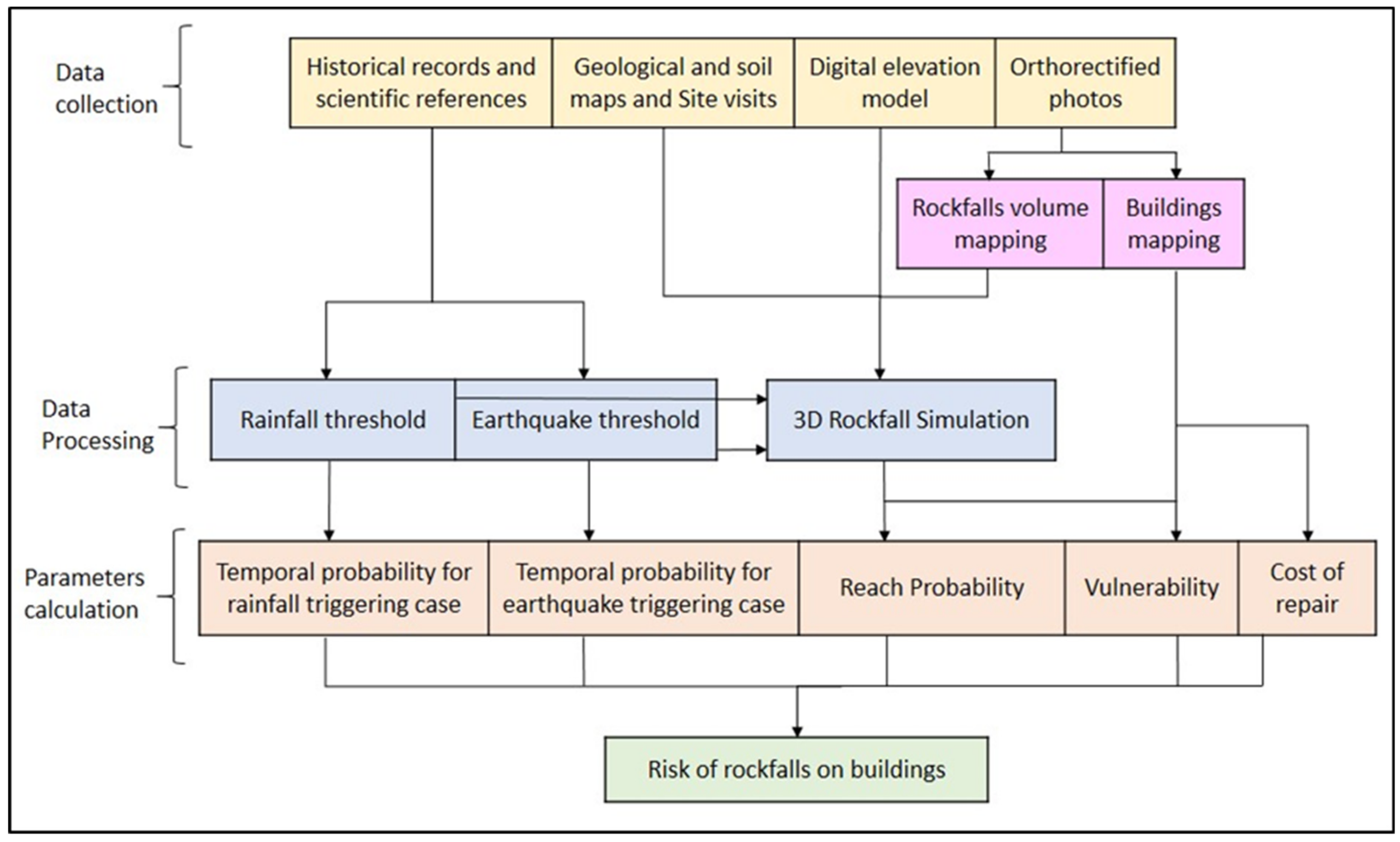
Figure 1. Flowchart representing the methodology.
J 07 00011 g001
Figure 2. Map of the study area showing RF distribution, RF release areas, fallen rock sizes, maximum observed reaching point, and location of buildings (built before and after the year 2000).
J 07 00011 g002
Figure 3. Reach probability in earthquake case.
J 07 00011 g003
Figure 4. Reach probability in rainfall case.
J 07 00011 g004
Figure 5. Mean kinetic energy of rockfalls—the case of earthquake.
J 07 00011 g005
Figure 6. Mean kinetic energy of rockfalls—the case of rainfall.
J 07 00011 g006
Figure 7. Risk of rockfalls on buildings, in USD per annum—case of earthquake.
J 07 00011 g007
Figure 8. Risk of rockfalls on buildings, in USD per annum—case of rainfall.
J 07 00011 g008
Table 1. The estimation of RF intensity (Source: Singh et al. (2021) [8]).
Rockfall IntensityKinetic Energy:
E (KJ)
Proposed I Value
LowLess than 300.2
Moderate30–3000.6
HighMore than 3001
Disclaimer/Publisher’s Note: The statements, opinions and data contained in all publications are solely those of the individual author(s) and contributor(s) and not of MDPI and/or the editor(s). MDPI and/or the editor(s) disclaim responsibility for any injury to people or property resulting from any ideas, methods, instructions or products referred to in the content.