Abstract
Small-signal models of DC-DC converters are often based on a state-space averaging approach, from which both control-oriented and other frequency-domain characteristics, such as input or output impedance, can be derived. Updating these models when extending the converter by filters or non-trivial loads, or adding control loops, can become a tedious task, however. To simplify this potentially error-prone process, a modular modeling approach is being proposed in this article. It consists of small state-space models for certain building blocks of a converter system on the one hand, and standardized operations for connecting these subsystem models to an overall converter system model on the other hand. The resulting state-space system model builds upon a two-port converter description and allows the extraction of control-oriented and impedance characteristics at any modeling stage, be it open loop or closed loop, single converter or series connections of converters. The ease of creating more complex models enabled by the proposed approach is also demonstrated with examples comprising multiple control loops or cascaded converters.
1. Introduction
Small-signal modeling of DC-DC converters has been a subject of research for several decades now, resulting in two main families of modeling techniques: state-space averaging [1] and switch or circuit averaging [2,3]. State-space averaging has become a broadly used modeling approach for DC-DC converters [4], and is considered the most effective method for building small-signal models [5]. It continuously received extensions, for example, for converters in discontinuous conduction mode (DCM) [6,7] or variable-frequency operation [8], and new theoretical results to this day [9].
The typical workflow using state-space averaging (SSA) includes applying Laplace transform and deriving frequency-domain transfer functions characterizing input/output impedance or control-oriented behavior [10], which must then be maintained individually. Thus, whenever the converter is being extended, for example, by control loops, this leads to the tedious and potentially error-prone work of having to adapt all frequency-domain models separately [11]. Even worse, the underlying state-space model might have to be derived again if circuit elements (such as an input filter) are added to the converter. Basso [12] calls this the “pain of the SSA technique”.
For easier modeling, the idea of modular approaches has emerged in the last two decades, be it for single converters [13], or even working towards automatic modeling solutions for microgrids [14,15]. Building and analyzing models for multi-converter configurations has of course been of increasing interest since the advent of DC microgrids [4,16], but has been the subject of research long before, especially when studying converter interactions in a cascaded source-load setup [17,18,19]. Matters of particular interest are impedance analysis [11,20,21], implications for controller design [17,22,23] and, of course, stability [18,19,24]. It has been pointed out [25,26] that studying detailed dynamic interactions between source and load converters is important for stability analysis, going beyond constant power load assumptions.
Many existing studies adopt an inverse-hybrid two-port description of converters (also known as g-parameters) [27], which lends itself well to the behavioral modeling of converters and converter systems [28,29], especially in the case of unterminated converter models [30,31,32].
Departing from the prevalent approach of deriving individual frequency-domain transfer functions for the different aspects of converter (system) modeling, this article proposes creating and maintaining a single state-space model in the time domain. It encompasses both control-oriented and electrical characteristics in a two-port description with inverse-hybrid parameters (g-parameters), following existing good practice and enhanced by additional control inputs as necessary. Whenever needed, of course, all relevant frequency-domain transfer functions can easily be extracted at any modeling stage from this model, superseding the necessity of updating individual frequency-domain transfer functions.
In order to relieve the “SSA pain” when building larger models, standardized (and therefore less error-prone) operations are being proposed for attaching controllers, closing control loops and creating series-connections of converter subsystems. These subsystems can be passive circuits such as input filters, open-loop or controlled converters, or even series-connections of converters themselves. In that manner, the actual modeling effort is reduced to modeling smaller building blocks which can later on be reused and combined to create larger converter system models.
The remainder of this article is organized as follows: The general modeling approach is presented in Section 2. Modeling examples for building blocks such as passive components, converters and controllers are given in the Appendix A, Appendix B and Appendix C, respectively. From these ingredients, a complete model of a converter system can be built up incrementally. For this purpose, new model connection operations are introduced in Section 3 (adding control loops to converters) and Section 4 (series-connecting converter subsystems), which form the main contribution of this article. Finally, examples for modeling a multiloop-controlled converter and a two-stage converter system are presented in Section 6.
2. Modular Modeling Approach
2.1. Model for Passive Components
For passive components of a converter system, such as an input filter or an electrical load, the two-port state-space model is given in general form in (1). The number of state variables, and therefore the size of the matrices , , depends on the order of the respective system, that is, the number of storage elements.
Figure 1 illustrates the definition of input and output voltages and currents for a generic two-port system. Examples for modeling passive subsystems of a converter system are given in Appendix A.
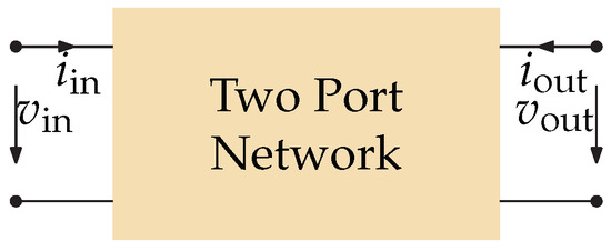
Figure 1.
Generic two-port network. Currents are defined as flowing into the input and output ports.
2.2. Model for Controlled Converters and Converter Systems
Based on Section 2.1, the model for a converter (system) gains at least one additional input: the control signal . For a single DC-DC converter, this will be the duty cycle in most cases. Equation (1) is therefore enhanced to (2). Examples are given or referenced in Appendix B.
Equation (2) is a very general model. Depending on both the approach for controlling the converter (such as voltage mode or current mode) as well as the modeling stage during the elaboration of the model, there are different possible meanings or functions the control signal can possess: duty ratio, peak or average current reference (in current mode control, if the model only describes the current loop so far), voltage reference (in voltage mode or if the outer voltage control loop around a current-controlled converter has been closed), or even the respective open-loop inputs if the control loop has not yet been closed in the model.
Additionally, (2) is very general in the regard that the model may contain a (series) connection of several controlled converters. In this case, is a vector containing the individual control loop inputs for the converters in this model.
When connecting input filters or loads to the model according to (2), its structure remains the same, therefore (2) is being used both for modeling “bare” converters as well as the final result, that is, a converter system with one or more controlled converters as well as possible filter and load subsystems.
2.3. Model for Controllers
While controllers—such as a controller for the output voltage or an underlying average current mode controller—will be modeled in this article in a state-space representation as well, they require a different treatment and do not fit into the two-port model category. This is due to the fact that even though the controllers may be realized in analog form by means of electric circuits, they represent an information flow rather than a power flow. The controller model employed here will be a continuous-time state-space model given in (3), with a single input (the control error value e) and a single output (the control signal u of the respective controller). Examples of controllers typically used for converters are given in Appendix C.
2.4. Making Connections
The most simple form of a practical converter system consists of the actual “bare” converter (such as a buck or boost converter), an (optional) input filter and a load, cf. Figure 2. A more complicated case arises when a second converter is attached as the load system of a first converter.

Figure 2.
Two-port network description consisting of three subsystems: input filter, converter (with a control input ), and the actual load.
In this article, a solution is presented to create a complete system model for arbitrary series connections of converter subsystems. The generic model ingredients have already been presented in Section 2.1 (passive components), Section 2.2 (converters), and Section 2.3 (controllers). Two different methods of connecting these model ingredients to a complete system mode are necessary: (1) connecting a converter with one or more controllers, which will be presented in Section 3, and (2) connecting (controlled) converter subsystems or passive subsystems in a series connection, which will be presented in Section 4.
A typical workflow of using the models and methods presented in this article is as follows: (1) create a converter model (examples in Appendix B), (2) create a controller model (examples in Appendix C) and connect the controller (Section 3) for every control loop of the converter, (3) make series connections to further controlled converters (if present, Section 4), (4) create models for input filter and load (examples in Appendix A) and connect them (Section 4). The latter may, of course, also be connected before connecting the controller in order to tune the controller according to possible interactions of the converter with source and load impedances, especially if the system consists only of a single converter.
3. Adding Control Loops to Converter Models
In the following, a general procedure is being described that combines a two-port converter model featuring one (scalar) control input as given in (2) with a model of the controller according to (3). Firstly, an open-loop model is being constructed, followed by the closed-loop model, both of which maintaining the same interface of the general two-port state-space model (2).
The control input of the given converter could be the duty cycle or the set-point of an inner control loop, such as an inner current control loop. Through the stages of connecting the converter model with the controller model, the meaning of the model’s control input changes from its original meaning to the control error value (open-loop case) and finally the set-point (reference signal) of the closed control loop. The interfaces of the respective two-port models are shown in Figure 3.
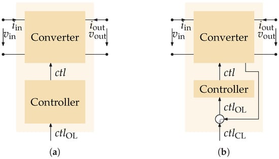
Figure 3.
Interfaces of the two-port network models with control inputs when adding a controller to a converter. (a) Open-loop case. (b) Closed-loop case.
In order to obtain the open-loop model, the state variable vector of the converter model must be enhanced by the state variables of the controller model. In general, a common model structure of the open-loop and closed-loop models can be given as follows in (4), with subscripts OL and CL distinguishing the open-loop and closed-loop case.
The main step required to obtain the , , , matrices of the open-loop model is to account for the changed meaning of the control input of the model. The (now internal) control input of the converter must be connected to the output of the controller, cf. (5).
In (5), n refers to the number of state variables in the converter model, and m to the number of state variables in the controller model.
When deriving the closed-loop model in the following, it will be assumed that there is no (or only a negligible) direct feedthrough from the original control input to the desired control variable. If, for example, the output voltage is the desired control variable, should hold, which is the case for all converter types mentioned in this article.
The , , matrices of the open-loop and closed-loop case are identical, that is, , , . The matrix of the closed-loop model is computed via (6), which is an equation known from classical state feedback control.
A suitable feedback gain matrix must be chosen depending on which control loop is being closed, such as an inner average current loop or an output voltage loop. It is important to note that is not being used to design the controller (as in state feedback control), but only to select and feed back the desired control variable when constructing the closed-loop state-space model. The controller parameters are contained in the controller model (3). To demonstrate that the choice of is almost trivial in most applications, the (probably) most important two cases will be shown in Section 3.1 and Section 3.2.
As a final side note, a sensor or filter with non-negligible dynamics in the feedback path can rather easily be accounted for by extending the converter model with the respective dynamics and choosing the output of the sensor or filter as the control variable.
3.1. Average Current Mode
For closing a current loop, must be chosen in order to extract the desired current variable from the vector of converter system states and feed it back to the third input of the open-loop converter model, that is, . If we, for example, assume for the converter model that the average current is the first state variable (as in the boost converter example in Appendix B.2), simply has to be chosen as (7).
3.2. Voltage Mode or Outer Voltage Loops
If output voltage is the desired control variable, which is the case for voltage mode as well as for an outer voltage loop around a current-controlled converter, has to be chosen as (8).
This assumes that holds for the uncontrolled converter model, which means that can approximately be extracted from the state variable vector by .
4. Connecting Converter Models
In order to create a combined state-space model for a series connection of two subsystems (denoted “source” and “load” here), the respective models for source (superscript S) and load (superscript L) must be given in the following form:
Note that the connection operation introduced in this section works regardless of the number of control inputs in the source and load models, that is, even without control inputs, as is the case for passive subsystems such as filters or loads. In these cases, the respective columns of the and matrices must simply be left out in all of the following equations.
The input and output ports of the combined system are the input port of the source subsystem and the output port of the load subsystem, that is, the following equations hold: , , , and , cf. Figure 4. The result is the following combined model (10).

Figure 4.
Series connection of two two-port networks (source and load). The control inputs are optional and only present if source or load contain at least one converter, respectively.
The equations of the resulting model can be found by replacing the inner terminal variables of the two-port series connection, which are not present in (10) anymore, cf. Figure 4. For the inner voltage and the inner current the following equations hold:
Putting (11) and (12) in the source/load state equations of (9) will now lead to the combined state equations in (10). Similarly, the output equation of the connected system in (10) is obtained by putting (11) and (12) in the output equations from (9) for and . The resulting detailed formulation of the matrix contents for , , , in (10) is given in (13).
It has to be noted that (13) will often be reduced to a simpler form in practical cases since not all matrix elements of the subsystem matrices are non-zero. Furthermore, (10) and (13) are primarily meant to be implemented in a computer algebra system or a numerical software package only once and then be used to conveniently build up a complete model of a DC-DC converter system from simple subsystems in a fully or semi-automated manner. Compact matrix formulations for (13) can be found by inspection, the corresponding set of equations is presented in (14).
5. Summary of the Building-Block Modeling Approach
For convenience, all building block types and connection operations of the modular modeling approach presented in this article are summarized in this section. Furthermore, the relation of the developed state-space model to well-known frequency-domain models of converter systems is given.
5.1. Building Block Types
To start with modeling a DC-DC converter or converter system, the first step is to collect all building blocks, such as models for the bare converter, controllers, filters, loads and so forth. In the modeling approach presented in this article, there are three different categories of building blocks in terms of their state-space model representation. For convenience, they are listed again in Table 1. Concrete examples for these three building block types are given in the Appendix A, Appendix B and Appendix C.

Table 1.
Summary of building block types in terms of their state space equation structure.
5.2. Connecting Building Blocks
There are two different kinds of connections that can be made in order to create a converter system model from smaller building blocks:
- Connecting converters with passive components or other converters. Since both building blocks for passive elements as given by (1) and building blocks for converters as given by (2) are two-port models, the same connection operation can be used for all these cases. The resulting model (10) is obtained by applying (13).
- Creating control loops. Connecting a controller, that is, a building block type as given by (3), to a converter is done by creating an open-loop model (4) using (5). For closing the control loop, the model’s matrix must be adapted using (6), with a feedback gain matrix chosen depending on the controlled variable, for example, one of (7) or (8) for current or voltage mode control.
All resulting models (connected subsystems, open- or closed-loop models) are of the same structure as the generic model (2), which means that frequency-domain characteristics as listed in the following section can be extracted at any modeling stage.
Since the structure and linearity of the resulting state-space models are preserved by the connection operations, there is no impact on the small-signal modeling accuracy of the building blocks.
5.3. Frequency-Domain Analysis
As mentioned before, one major benefit of the modular state-space modeling approach presented in this article is that, when needed, frequency-domain transfer functions can easily be obtained at any modeling stage. Table 2 lists all frequency-domain models that can be extracted from the generic converter or converter system model (2), regardless of the current modeling state (e.g., with or without closed-loop control, with or without filters and loads etc.).

Table 2.
Transfer functions than can be obtained from the converter (system) model (2), cf. Section 2.2, at any modeling stage (e.g., with or without controller).
6. Examples
In the following, three modular modeling examples are presented with special emphasis on demonstrating the systematic methods to extend two-port oriented state-space models of converters with control loops (method from Section 3, example in Section 6.1) and to create an overall model from series-connections of subsystems (method from Section 4, examples in Section 6.2 and Section 6.3).
It should be noted that the parameterization of converters and controllers in this section was chosen rather arbitrarily and solely to serve as numerical examples for the modeling methods developed here. For simplicity, all inductors and capacitors in the following examples are being modeled with a uniform equivalent series resistance (ESR) value of mΩ, unless otherwise noted.
As will be demonstrated, all models developed in these examples can be constructed from already available modules, thus no manual effort is required regarding the derivation of state-space equations. In order to illustrate the validity of the models in an intuitive manner, comparisons will be provided with time-domain results from circuit simulations.
6.1. Buck Converter with Multiloop (I2) Control
The systematic approach to extend a converter model by attaching a control loop (presented in Section 3) opens up the possibility of studying characteristics of converters with multiple control loops in an easy manner. Therefore, as a first example, a buck converter in peak current mode control will be examined, which will be extended by a second control loop for the average current (also known as I2 control [33]) and a third outer voltage control loop. Only three steps are necessary to create the complete model from already available building blocks:
- As the starting point to build up the complete model, the two-port state-space model for the PCM buck converter from Reference [34] is being used. The example is parameterized as given in the following. Operating point: , , . Power stage: , , . Peak current mode controller: external ramp of per switching cycle.
- For the I2 current loop, an additional controller for the average inductor current is being added. A Type 1 controller with ,000 is employed, cf. Appendix C, which is connected to the state-space model as described in Section 3.1.
- For the outer voltage control loop, a Type 2 controller with zero at , pole at and is being used, cf. Appendix C. It is connected to the model as described in Section 3.2.
To validate the model in the time domain, it is being compared against a circuit simulation of this converter/controller configuration with three test cases. Firstly, a reference step of the I2 current control loop (i.e., using the model after step 2 as given above) is simulated using both the detailed circuit simulation and the transfer function for the control loop of the average inductor current, which can easily be obtained from the state-space model (transfer function from the control input to the state variable of the inductor current). The results are given in Figure 5 and confirm that the dynamics of the average inductor current under a combined average and peak current mode (I2) control are very well captured by the state-space model.
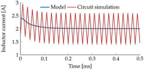
Figure 5.
Impact of a reference step at on the inductor current of the buck converter from example Section 6.1 with closed I2-current loop.
As a second test, a reference voltage step is performed using the outer voltage control loop (i.e., with the complete model after step 3). The results are given in Figure 6 and, again, the circuit simulation and state-space model agree very well.
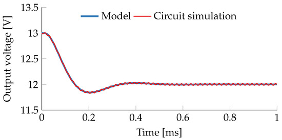
Figure 6.
Reference step at of the buck converter from example Section 6.1 with closed voltage loop and underlying I2 current control.
Finally, +25% load step is being applied. The results in Figure 7 once more confirm that the state-space model captures the dynamics of the converter under this multiloop control configuration very well.
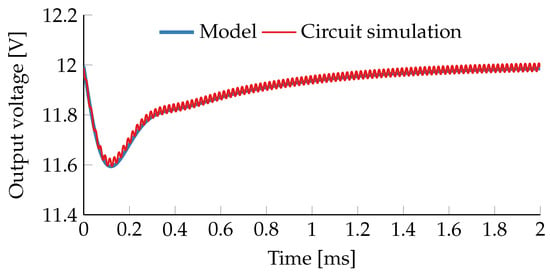
Figure 7.
Impact of a 25% load step at on the output voltage of the buck converter from example Section 6.1 with closed voltage loop.
Again, it should be noted that frequency-domain characteristics such as impedance plots or control-to-output transfer functions are all readily available at any stage of the state-space modeling procedure, cf. Table 2 but omitted here for brevity. There is no necessity anymore to derive custom models or transfer functions for the I2 current loop configuration, in contrast to existing work [33,35,36].
6.2. Boost Converter with Input Filter
With the model connection approach presented in Section 4, building up higher-order state-space models has become an easy task. As an example, the impact of additional input circuitry on a voltage mode controlled boost converter will be studied here. Four steps are necessary in order to obtain the final model from already available modules:
- A linearized state-space model for a boost converter in CCM as given in Appendix B.2. The example is parameterized as given in the following. Operating point: , , . Power stage: , , .
- A load resistance (model from Appendix A.1) corresponding to the operating point is connected at the converter output using Section 4.
- A Type 3 controller (cf. Appendix C) is being employed for the voltage control loop, with zeros placed at , poles at and , and . It is connected to the model as described in Section 3.2.
- Finally, an LC filter model (cf. Appendix A.2) accounting for both an input filter and wiring is connected at the input of the converter model using Section 4, with , , and .
As a first step, the influence of the input filter on the frequency-domain characteristics will be examined. The input and output impedance transfer functions can easily be obtained from our two-port oriented state-space model, cf. Table 2. Figure 8 shows the impedance magnitude and phase plots for the voltage mode controlled boost converter both with and without input filter. In the input impedance plots one can clearly notice the negative resistance behavior of the controlled converter at low frequencies. Furthermore one can, for instance, observe a dampening effect of the input filter around in the output impedance, which has an impact on load step dynamics.
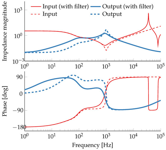
Figure 8.
Input and output impedance of the boost converter from example Section 6.2, with closed voltage loop, both with input filter (solid lines) and without input filter (dashed lines).
Therefore, a time-domain simulation of a +100% load step at the output will be performed with and without input filter and compared against the results of detailed time-domain circuit simulations. The results in Figure 9 not only confirm the good accuracy of the state-space model, but also clearly demonstrate the dampening effect of this particular input circuitry on the load step dynamics, as predicted in the frequency-domain analysis.
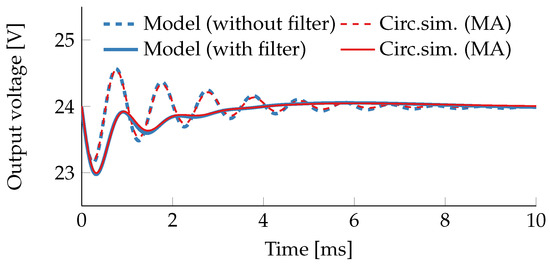
Figure 9.
Impact of a 100% load step at on the output voltage of the boost converter from example Section 6.2 with closed voltage loop, both with input filter (solid lines) and without input filter (dashed lines). For better comparability, the circuit simulation results were filtered (moving average) to remove the switching ripple voltage.
6.3. Series-Connected Boost and Buck Converter Stages
Since the model connection approach developed in Section 4 is not restricted to attaching subsystems with passive components, one can just as easily connect models of controlled converters in a source/load configuration. Therefore, as a final example, we will create a series-connected configuration of the boost and buck stages examined in Section 6.1 and Section 6.2, respectively, cf. Figure 10. The following (almost trivial) steps are required to obtain the complete model:

Figure 10.
Two-port view of a series connection of boost and buck converter stages. In both stages, the filter elements L and C are being modeled with equivalent series resistances (ESR).
- Reuse the final model from Section 6.2 (voltage-controlled boost converter including input filter) but without the load resistance, since the buck converter will constitute the new load to the boost stage.
- Reuse the final model from Section 6.1 (voltage-controlled buck converter with underlying I2 current control).
- Connect the buck converter model at the output of the boost converter, as described in Section 4.
As a small example of the possibilities offered by the all-encompassing state-space model, the interactions between the two power stages will be examined in the following test case. Again, a +25% load step is applied at the output of the buck stage and the impact on the intermediate output voltage of the boost stage is observed. From the state-space model, a transfer function from the output current (i.e., the load) to the state variable representing the output capacitor voltage of the boost stage can easily be extracted. It is, once more, being compared against a time-domain circuit simulation containing the series-connected converter configuration.
From the results in Figure 11 one can conclude that the overall state-space model is very well able to predict the essential dynamics. Since the buck stage has much faster dynamics than the boost stage, the load step dynamics in Figure 11 closely resemble Figure 9 in this case but it has to be emphasized again that the results in Figure 11 fully incorporate small-signal interactions of the two connected power stages with all their respective controllers.
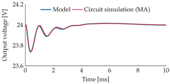
Figure 11.
Impact of a 25% output load step at of the series-connected buck stage from example Section 6.3 on the intermediate output voltage of the boost stage. For better comparability the circuit simulation result was filtered (moving average) to remove the switching ripple voltage.
7. Conclusions
The rederivation of state-space models of converter systems when adding input filters or non-trivial loads such as other converters was, up to now, considered a painful process [12]—and rightfully so. With the systematic approach of extending such state-space models presented in this article, adding control loops and building up system models from series-connected modules such as filters, loads, or converters have become straightforward tasks.
This modular approach leverages already existing models for common converter or filter topologies by incorporating them as building blocks, such that users do not have to manually derive larger sets of state-space equations anymore in many application cases. If not yet available, the modeling efforts required are only limited to the respective subsystem.
The small-signal modeling accuracy of the building blocks is not compromised by the proposed connection operations, the resulting models in all modeling stages preserve their structure and always remain linear.
The validity of the resulting small-signal models has been illustrated and compared in the time-domain against circuit simulations.
At all stages of the modeling procedure proposed in this article, the benefits of a two-port oriented state-space description become obvious, since input/output impedance and control-to-output or control-to-state transfer functions are easily obtainable from one single model. This also allows for the design of controllers starting from the innermost loop in a systematic fashion, while incorporating interactions with non-trivial source or load elements.
Funding
This research received no external funding.
Conflicts of Interest
The author declares no conflict of interest.
Appendix A. Building Blocks: Passive Component Models
The generic two-port modeling approach for passive subsystems of a converter system has already been introduced in Section 2.1. In this section, two typical examples often found in a converter system will be given: an (ideal) resistive load, and an LC input filter. These are also used in the examples presented in Section 6.
Appendix A.1. Resistive Load
Appendix A.2. LC Filter
In (A2), the two-port state-space model of an LC filter as depicted in Figure A1b is being given. In addition to the circuit in Figure A1b, the effects of equivalent series resistances (ESR) in both inductor (ESR ) and capacitor (ESR ) have been accounted for in (A2).

Figure A1.
Two-port network subsystems for passive elements. (a) Resistive load. (b) LC filter.
As a side note it can be stated that manually creating a model for a two-stage LC filter is not necessary. A benefit of the connection method presented in Section 4 will be that one can create a series connection of two LC filter models from (A2) if that is necessary.
More generally speaking: it is beneficial to create very simple building blocks as demonstrated in this section, and bypass the error-prone process of manually modeling a larger system by creating a complete system model from the combination of these small subsystems instead. The necessary tools are presented in Section 4.
Appendix B. Building Blocks: Converter Models
Appendix B.1. Available Converter Models
The two-port state-space approach to converter modeling goes beyond most state-space models found in the literature, which mostly do not account for the output current as an additional input variable of the model. This is probably due to the fact that state-space models have so far mostly been used only as an intermediate step in order to derive transfer functions in frequency domain.
Nevertheless, a variety of two-port oriented state-space models can already be found in more recent work, and these can be used here almost in a plug-and-play fashion. For example, models for buck, boost, and flyback converter in peak current mode (PCM) control, all in continuous conduction mode (CCM), are presented in [34]; and PCM-controlled buck and boost converters in DCM in [37,38], respectively. Furthermore, ready-to-use state-space models for buck, boost, and buck-boost converters can be found in [39,40], which have to be seen as the most comprehensive references devoted to systematic two-port modeling of converters.
In this article, the recommended strategy is to model the load subsystem of the converter separately (cf. Appendix A), and connect it to the converter models afterwards (cf. Section 4). This implies that, ideally, the converter modeled with (2) should be unterminated at first. However, most state-space converter models found in the literature do feature a resistive load, but these can be used here by letting , as done e.g., in [41]. The models presented in [39] do already describe unterminated converters.
Appendix B.2. Example: Boost Converter
For an unterminated boost converter operating in CCM (cf. Figure A2), the , , , matrices for a linearized state-space model (2) with small simplifications (e.g., ideal switches) are given in (A3). The power stage inductor L and capacitor C are being modeled with ESR values and . D, , and define the operating point for the duty cycle, the average inductor current, and the output voltage, respectively. The two state variables are the inductor current and the output capacitor voltage , i.e., .
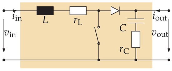
Figure A2.
Two-port view of an unterminated boost converter stage.
This model is also used and compared against time-domain circuit simulations in the examples presented in Section 6.2 (boost converter with input filter) and Section 6.3 (series-connected boost and buck stages).
Appendix C. Building Blocks: Controller Models
For the control of voltage and current in power converters, some of the most prominent examples of controllers used in practice besides proportional-integral controllers are the so-called Type 1, Type 2, and Type 3 controllers described in [42,43]. These are integral controllers with zero, one, or two lead-lag elements, respectively, and are also being used in the examples in Section 6.
In Table A1, transfer functions and state-space models according to (3) are given for these controller types. For all of them, the state-space models do not possess direct feedthrough terms in (3), i.e., .

Table A1.
Transfer function and state-space model matrices , , according to (3) for controllers known as Type 1, 2, and 3.
Table A1.
Transfer function and state-space model matrices , , according to (3) for controllers known as Type 1, 2, and 3.
| Type 1 | Type 2 | Type 3 |
|---|---|---|
References
- Middlebrook, R.D.; Ćuk, S. A General Unified Approach to Modelling Switching-Converter Power Stages. In Proceedings of the 1976 IEEE Power Electronics Specialists Conference, Cleveland, OH, USA, 8–10 June 1976; pp. 18–34. [Google Scholar] [CrossRef]
- Vorpérian, V. Simplified Analysis of PWM Converters Using Model of PWM Switch. Part I: Continuous Conduction Mode. IEEE Trans. Aerosp. Electron. Syst. 1990, 26, 490–496. [Google Scholar] [CrossRef]
- Czarkowski, D.; Kazimierczuk, M.K. Energy-Conservation Approach to Modeling PWM DC-DC Converters. IEEE Trans. Aerosp. Electron. Syst. 1993, 29, 1059–1063. [Google Scholar] [CrossRef]
- Francés, A.; Asensi, R.; García, O.; Prieto, R.; Uceda, J. Modeling Electronic Power Converters in Smart DC Microgrids—An Overview. IEEE Trans. Smart Grid 2018, 9, 6274–6287. [Google Scholar] [CrossRef]
- Zhan, D.; Wei, L.; Zhang, Y.; Yao, Y. A Generalized Model of Nonisolated Multiphase DC-DC Converter Based on Novel Switching Period Averaging Method. IEEE Trans. Power Electron. 2015, 30, 5181–5191. [Google Scholar] [CrossRef]
- Davoudi, A.; Jatskevich, J.; De Rybel, T. Numerical State-Space Average-Value Modeling of PWM DC-DC Converters Operating in DCM and CCM. IEEE Trans. Power Electron. 2006, 21, 1003–1012. [Google Scholar] [CrossRef]
- Sun, J.; Mitchell, D.M.; Greuel, M.F.; Krein, P.T. Averaged Modeling of PWM Converters Operating in Discontinuous Conduction Mode. IEEE Trans. Power Electron. 2001, 16, 482–492. [Google Scholar] [CrossRef]
- Priewasser, R.; Agostinelli, M.; Unterrieder, C.; Marsili, S.; Huemer, M. Modeling, Control, and Implementation of DC-DC Converters for Variable Frequency Operation. IEEE Trans. Power Electron. 2014, 29, 287–301. [Google Scholar] [CrossRef]
- Meo, S.; Toscano, L. Some New Results on the Averaging Theory Approach for the Analysis of Power Electronic Converters. IEEE Trans. Ind. Electron. 2018, 65, 9367–9377. [Google Scholar] [CrossRef]
- Petrović, T.B.; Rakić, A.Ž. Linear Robust Approach to DC/DC Converter Modeling—I: Deterministic Switching. Electr. Eng. 2004, 86, 267–273. [Google Scholar] [CrossRef]
- Vesti, S.K.; Suntio, T.; Oliver, J.Á.; Prieto, R.; Cobos, J.A. Effect of Control Method on Impedance-Based Interactions in a Buck Converter. IEEE Trans. Power Electron. 2013, 28, 5311–5322. [Google Scholar] [CrossRef]
- Basso, C. Switch-Mode Power Supplies: SPICE Simulations and Practical Designs, 2nd ed.; McGraw-Hill: New York, NY, USA, 2014. [Google Scholar]
- Wu, T.F.; Chen, Y.K. Modeling PWM DC/DC Converters out of Basic Converter Units. IEEE Trans. Power Electron. 1998, 13, 870–881. [Google Scholar] [CrossRef]
- Francés, A.; Asensi, R.; García, O.; Prieto, R.; Uceda, J. A Black-box Modeling Approach for DC Nanogrids. In Proceedings of the 2016 IEEE Applied Power Electronics Conference and Exposition (APEC), Long Beach, CA, USA, 20–24 March 2016; pp. 1624–1631. [Google Scholar] [CrossRef]
- Francés, A.; Asensi, R.; García, O.; Prieto, R.; Uceda, J. How to Model a DC Microgrid: Towards an Automated Solution. In Proceedings of the 2017 IEEE Second International Conference on DC Microgrids (ICDCM), Nuremburg, Germany, 27–29 June 2017; pp. 609–616. [Google Scholar] [CrossRef]
- Haghmaram, R.; Sedaghati, F.; Ghafarpour, R. Power Exchange Among Microgrids using Modular-Isolated Bidirectional DC-DC Converter. Electr. Eng. 2017, 99, 441–454. [Google Scholar] [CrossRef]
- Haroun, R.; Cid-Pastor, A.; Aroudi, A.E.; Martíinez-Salamero, L. Synthesis of Canonical Elements for Power Processing in DC Distribution Systems Using Cascaded Converters and Sliding-Mode Control. IEEE Trans. Power Electron. 2014, 29, 1366–1381. [Google Scholar] [CrossRef]
- Li, H.; Shang, J.; You, X.; Zheng, T.; Zhang, B.; Lü, J. A Novel Stability Analysis Method Based on Floquet Theory for Cascaded DC-DC Converters System. In Proceedings of the 2015 IEEE Energy Conversion Congress and Exposition (ECCE), Montreal, QC, Canada, 20–24 September 2015; pp. 2679–2683. [Google Scholar] [CrossRef]
- Mummadi, V.; Singamaneni, B.S. Stability Analysis of Cascaded DC-DC Power Electronic System. IEEJ Trans. Electr. Electron. Eng. 2009, 4, 763–770. [Google Scholar] [CrossRef]
- Ahmadi, R.; Ferdowsi, M. Modeling Closed-Loop Input and Output Impedances of DC-DC Power Converters Operating Inside DC Distribution Systems. In Proceedings of the 2014 IEEE Applied Power Electronics Conference and Exposition (APEC), Fort Worth, TX, USA, 16–20 March 2014; pp. 1131–1138. [Google Scholar] [CrossRef]
- Ali, H.; Zheng, X.; Zaman, H.; Liu, H.; Wu, X. Behavioral Modeling for Parallel- and Cascade-Connected DC-DC Converters. J. Circuits Syst. Comput. 2018. [Google Scholar] [CrossRef]
- Ahmadi, R.; Ferdowsi, M. Controller Design Method for a Cascaded Converter System Comprised of Two DC-DC Converters Considering the Effects of Mutual Interactions. In Proceedings of the 2012 Twenty-Seventh Annual IEEE Applied Power Electronics Conference and Exposition (APEC), Orlando, FL, USA, 5–9 February 2012; pp. 1838–1844. [Google Scholar] [CrossRef]
- Pidaparthy, S.K.; Choi, B. Control Design and Loop Gain Analysis of DC-to-DC Converters Intended for General Load Subsystems. Math. Probl. Eng. 2015. [Google Scholar] [CrossRef]
- Ahmadi, R.; Paschedag, D.; Ferdowsi, M. Analyzing Stability Issues in a Cascaded Converter System Comprised of Two Voltage-Mode Controlled DC-DC Converters. In Proceedings of the 2011 Twenty-Sixth Annual IEEE Applied Power Electronics Conference and Exposition (APEC), Fort Worth, TX, USA, 6–11 March 2011; pp. 1769–1775. [Google Scholar] [CrossRef]
- Cupelli, M.; Zhu, L.; Monti, A. Why Ideal Constant Power Loads Are Not the Worst Case Condition From a Control Standpoint. IEEE Trans. Smart Grid 2015, 6, 2596–2606. [Google Scholar] [CrossRef]
- Tehrani, H.M.; Francés, A.; Asensi, R.; Uceda, J. A Comparison of Stability Analysis of Constant Power Load with Detailed Model in DC Microgrids. In Proceedings of the 2018 7th International Conference on Renewable Energy Research and Applications (ICRERA), Paris, France, 14–17 October 2018; pp. 487–493. [Google Scholar] [CrossRef]
- Maranesi, P.G.; Tavazzi, V.; Varoli, V. Two-port Characterization of PWM Voltage Regulators at Low Frequencies. IEEE Trans. Ind. Electron. 1988, 35, 444–450. [Google Scholar] [CrossRef]
- Suntio, T.; Viinamäki, J.; Jokipii, J.; Messo, T.; Kuperman, A. Dynamic Characterization of Power Electronic Interfaces. IEEE J. Emerg. Sel. Top. Power Electron. 2014, 2, 949–961. [Google Scholar] [CrossRef]
- Zenger, K.; Altowati, A.; Suntio, T. Dynamic Properties of Interconnected Power Systems—A System Theoretic Approach. In Proceedings of the 2006 1st IEEE Conference on Industrial Electronics and Applications, Singapore, 24–26 May 2006; pp. 1–6. [Google Scholar] [CrossRef]
- Arnedo, L.; Burgos, R.; Boroyevich, D.; Wang, F. System-Level Black-Box DC-to-DC Converter Models. In Proceedings of the 2009 Twenty-Fourth Annual IEEE Applied Power Electronics Conference and Exposition (APEC), Washington, DC, USA, 15–19 February 2009; pp. 1476–1481. [Google Scholar] [CrossRef]
- Cvetkovic, I.; Boroyevich, D.; Mattavelli, P.; Lee, F.C.; Dong, D. Unterminated Small-Signal Behavioral Model of DC-DC Converters. IEEE Trans. Power Electron. 2013, 28, 1870–1879. [Google Scholar] [CrossRef]
- Suntio, T. On Dynamic Modeling of PCM-Controlled Converters—Buck Converter as an Example. IEEE Trans. Power Electron. 2018, 33, 5502–5518. [Google Scholar] [CrossRef]
- Yan, Y.; Lee, F.C.; Mattavelli, P.; Liu, P.H. I2 Average Current Mode Control for Switching Converters. IEEE Trans. Power Electron. 2014, 29, 2027–2036. [Google Scholar] [CrossRef]
- Smithson, S.C.; Williamson, S.S. A Unified State-Space Model of Constant-Frequency Current-Mode Controlled Power Converters in Continuous Conduction Mode. IEEE Trans. Ind. Electron. 2015, 62, 4514–4524. [Google Scholar] [CrossRef]
- He, S.; Hung, J.Y.; Nelms, R.M. Small-Signal Modeling of I2 Average Current Mode Control. IEEE Trans. Power Electron. 2016, 31, 3849–3858. [Google Scholar] [CrossRef]
- Li, R.; Seto, K.; Kiefer, J.; Li, S. Analysis, Simulation and Experimental Evaluation of Constant-Frequency Trailing-Edge-Modulated I2 Average Current-Mode Control. In Proceedings of the 2016 IEEE 8th International Power Electronics and Motion Control Conference (IPEMC-ECCE Asia), Hefei, China, 22–26 May 2016; pp. 2077–2084. [Google Scholar] [CrossRef]
- Suntio, T. Dynamic Modeling and Analysis of PCM-Controlled DCM-Operating Buck Converters—A Reexamination. Energies 2018, 11, 1267. [Google Scholar] [CrossRef]
- Suntio, T. Modeling and Analysis of a PCM-Controlled Boost Converter Designed to Operate in DCM. Energies 2019, 12, 4. [Google Scholar] [CrossRef]
- Suntio, T. Dynamic Profile of Switched-Mode Converter: Modeling, Analysis and Control; Wiley-VCH: Weinheim, Germany, 2009. [Google Scholar]
- Suntio, T.; Messo, T.; Puukko, J. Power Electronic Converters: Dynamics and Control in Conventional and Renewable Energy Applications; Wiley-VCH: Weinheim, Germany, 2017. [Google Scholar]
- Suntio, T. Unified Average and Small-Signal Modeling of Direct-On-Time Control. IEEE Trans. Ind. Electron. 2006, 53, 287–295. [Google Scholar] [CrossRef]
- Venable, H.D. Optimum Feedback Amplifier Design for Control Systems; Venable Technical Paper #3; Venable Industries: Austin, TX, USA, 1986. [Google Scholar]
- Basso, C. Designing Control Loops for Linear and Switching Power Supplies: A Tutorial Guide; Artech House: Boston, MA, USA, 2012. [Google Scholar]
© 2019 by the author. Licensee MDPI, Basel, Switzerland. This article is an open access article distributed under the terms and conditions of the Creative Commons Attribution (CC BY) license (http://creativecommons.org/licenses/by/4.0/).