Research on K-Value Selection Method of K-Means Clustering Algorithm

Abstract

Among many clustering algorithms, the K-means clustering algorithm is widely used because of its simple algorithm and fast convergence. However, the K-value of clustering needs to be given in advance and the choice of K-value directly affect the convergence result. To solve this problem, we mainly analyze four K-value selection algorithms, namely Elbow Method, Gap Statistic, Silhouette Coefficient, and Canopy; give the pseudo code of the algorithm; and use the standard data set Iris for experimental verification. Finally, the verification results are evaluated, the advantages and disadvantages of the above four algorithms in a K-value selection are given, and the clustering range of the data set is pointed out.

1. Introduction

Cluster analysis is one of the most important research directions in the field of data mining. “Things are clustered and people are grouped”; compared with other data mining methods, clustering can complete the classification of data without prior knowledge. Clustering algorithms can be divided into multiple types based on partitioning, density, and model [1]. A clustering algorithm is a process of dividing a physical or abstract object into a collection of similar objects. A cluster is a collection of data objects; objects in the same cluster are like each other and different from objects in other clusters [2]. For a clustering task, we want to get the objects as close as possible within the clusters: first cluster tends to sample or data point. However, the randomness of sample center point selection tends to make cluster aggregation not converge. Cluster analysis is based on the similarity in clustering data sets, which is unsupervised learning.

In the partition-based clustering algorithm, K-means algorithm has many advantages such as simple mathematical ideas, fast convergence, and easy implementation [3]. Therefore, the application fields are very broad, including different types of document classification, music, movies, classification based on user purchase behavior, the construction of recommendation systems based on user interests, and so on. With the increase of the amount of data, the traditional K-means algorithm has been difficult to meet the actual needs when analyzing massive data sets. In view of the shortcomings of the traditional K-means algorithm, many scholars have proposed improvement measures based on K-means. For instance, in Reference [4], a simple and efficient implementation of the K-means clustering algorithm is presented to solve the problem of the cluster center point not being well-determined; it built a kd-tree data structure for the data points. The algorithm is easy to implement and can effectively avoid entering the local optimal solution to some extent. For the problems of the traditional clustering algorithms having no way to take advantage of some background knowledge (about the domain or the data set), an Improved K-means Algorithm Based on Multiple Information Domains is presented in Reference [5]; they apply this method to six data sets and the real-world problem of automatically detecting road lanes from global positioning system (GPS) data. Experiments show that the improved algorithm is more correct when selecting K values when solving practical problems. Two algorithms which extend the k-means algorithm to categorical domains and domains are reported in Reference [6], through the pattern mixing algorithm, the combination of the effectiveness measure, in order to solve the problem of complex data and more noise in the real world. A principal Component Analysis (PCA) method is implemented in Reference [7]; they use the artificial neural network (ANN) algorithm and K-nearest neighbor (KNN) and support vector machine (SVM) classification algorithms to extract and analyze the features, which effectively realize the classification of malware. The clustering algorithm is also applied to the early detection of pulmonary nodules [8]; they propose a novel optimized method of feature selection for both cluster and classifier components. In the field of medical imaging, clustering and classification based on selection features effectively improve the classification performance of Computer-aided detection (CAD) systems. With the advent of deep learning methods in pattern recognition applications, some scholars have applied them to cluster analysis. For example, in Reference [9], by studying the performance of a CAD system for lung nodules in Computed tomography (CT) as a function of slice thickness, a method of comparing the performance of CAD systems using a training method using nonuniform data was proposed.

In summary, based on the traditional K-means clustering algorithm, this paper discusses how to quickly determine the K-value algorithm. The remainder of this paper is organized as follows: Section 2 provides a brief description of the K-means clustering algorithm. Section 3 presents the four K-value selection algorithms—Elbow Method, Gap Statistic, Silhouette Coefficient and Canopy—and elucidates the various methods with sample data along with their experimental results. Finally, a discussion and conclusions are given in Section 4.

2. The K-means Algorithm

The K-means algorithm is a simple iterative clustering algorithm. Using the distance as the metric and given the K classes in the data set, calculate the distance mean, giving the initial centroid, with each class described by the centroid. For a given data set X containing n multidimensional data points and the category K to be divided, the Euclidean distance is selected as the similarity index and the clustering targets minimize the sum of the squares of the various types; that is, it minimizes [10]

$$\mathrm{d}={\displaystyle \sum }_{k=1}^k{\displaystyle \sum }_{i=1}^n||(x_i-u_k)||{}^2$$

(1)

where k represents K cluster centers, $u_k$ represents the kth center, and $x_i$ represents the ith point in the data set. The solution to the centroid $u_k$is as follows:

$$\begin{array}{ll}\frac{\partial }{\partial u_k}& =\frac{\partial }{\partial u_k}{\displaystyle {\displaystyle \sum }_{k=1}^k}{\displaystyle {\displaystyle \sum }_{i=1}^n}{\left(x_i-u_k\right)}^2\\ & ={\displaystyle {\displaystyle \sum }_{k=1}^k}{\displaystyle {\displaystyle \sum }_{i=1}^n}\frac{\partial }{\partial u_k}{\left(x_i-u_k\right)}^2\\ & ={\displaystyle {\displaystyle \sum }_{i=1}^n}2(x_i-u_k)\end{array}$$

(2)

Let Equation (2) be zero; then$u_k=\frac{1}{n}{\displaystyle \sum }_{i=1}^n{x}_i$.

The central idea of algorithm implementation is to randomly extract K sample points from the sample set as the center of the initial cluster: Divide each sample point into the cluster represented by the nearest center point; then the center point of all sample points in each cluster is the center point of the cluster. Repeat the above steps until the center point of the cluster is unchanged or reaches the set number of iterations. The algorithm results change with the choice of the center point, resulting in an instability of the results. The determination of the central point depends on the choice of the K value, which is the focus of the algorithm; it directly affects the clustering results, such as the local optimality or global optimality [11].

3. Research on K-Value Selection Algorithm

For the K-means algorithm, the number of clusters depends on the K-value setting [12]. In practice, the K value is generally difficult to define. The choice of K value directly determines the data cluster that needs to be clustered into multiple clusters. At the beginning of the algorithm, people use the “shooting the head” method to determine the K value, which is estimated to later give many improvements proposed for optimization algorithms. This paper mainly summarizes the methods of K-value selection with certain representativeness and gives further analysis and experimental verification. The experimental simulation environment is Intel Core i5 dual-core [email protected], 4G memory, 500G hard disk space.

The experiment used the UCI Machine Learning Repository machine to learn the Iris data set in the data set [13]. The Iris data set consists of three classes, each with 50 elements, a total of 150 samples, and four attributes per sample, with each representing a type of iris.

In order to have a more obvious clustering effect to test the pros and cons of the K-value algorithm, the latter two dimensions of the Iris data set sample are selected during the experiment.

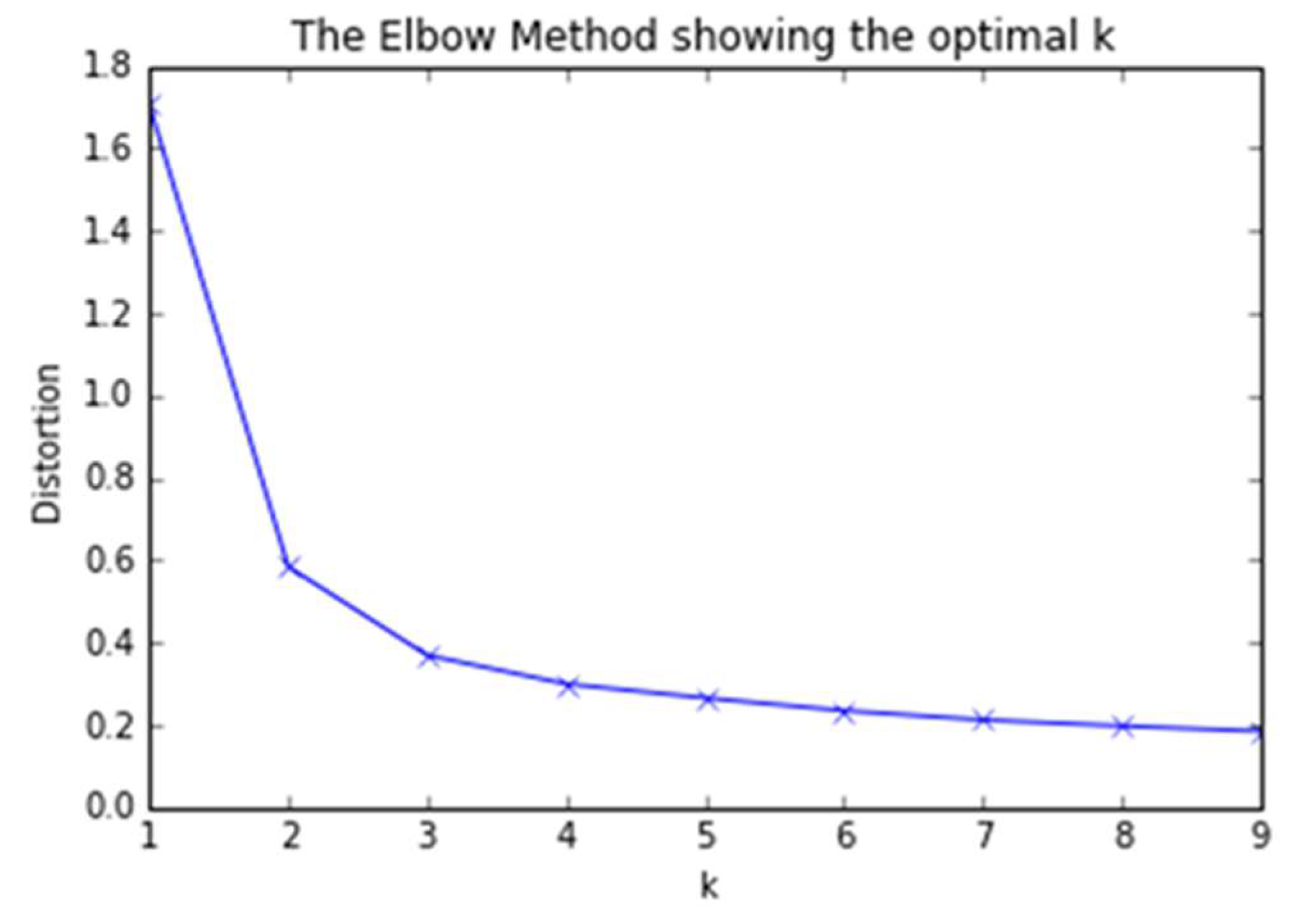
3.1. An Elbow Method Algorithm

The basic idea of the elbow rule is to use a square of the distance between the sample points in each cluster and the centroid of the cluster to give a series of K values. The sum of squared errors (SSE) is used as a performance indicator. Iterate over the K-value and calculate the SSE. Smaller values indicate that each cluster is more convergent.

When the number of clusters is set to approach the number of real clusters, SSE shows a rapid decline. When the number of clusters exceeds the number of real clusters, SSE will continue to decline but it will quickly become slower. The pseudo code of the algorithm is as follows:

Algorithm 1: Silhouette Coefficient

Input: iris = datasets.load_iris(), X = iris.data [:, 2 :]

Output: d, k

1: d = [];

2: for k = 1, k in rang (1, 9) do

$3:d={\displaystyle \sum }_{i=1}^k\sum dist{\left(x,c_i\right)}^2$;

4: return d, k;

The K value can be better determined by plotting the K-SSE curve and by finding the inflection point down. As shown in Figure 1, there is a very obvious inflection point when K = 2, so when the K value is 2, the data set clustering effect is the best, as shown in Figure 2.

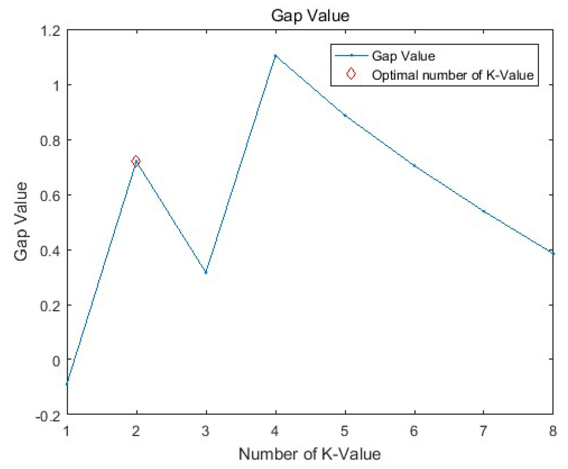
3.2. The Gap Statistic Algorithm

Gap Statistic is an algorithm proposed by Tibshirani [14] to determine the number of clusters of data sets with unknown classification numbers. The basic idea of Gap Statistic is to introduce reference measurements, which can be obtained by the Monte Carlo sampling method [15] and to calculate the sum of the squares of the Euclidean distance between two measurements in each class. The clustering results of the constructed reference zero-mean distribution are compared to determine the optimal number of clusters in the data set. It is calculated as follows:

$$\begin{array}{ll}Ga{p}_n\left(k\right)& =E_n^{*}\left(\log \left(W_k\right)\right)-log{W}_k{E}_n^{*}(\log \left(W_k\right))\\ & =\left(\raisebox{1ex}{$1$}\!\left/ \!\raisebox{-1ex}{$P$}\right.\right){\displaystyle {\displaystyle \sum }_{b=1}^P}\log (W_{kb}^{*})\approx \left(\raisebox{1ex}{$1$}\!\left/ \!\raisebox{-1ex}{$P$}\right.\right){\displaystyle {\displaystyle \sum }_{b=1}^P}\log (W_{kb}^{*})s\left(k\right)\\ & =\sqrt{\frac{1+P}{P}}s\left(k\right)\end{array}$$

(3)

where $E_n^{*}\left(\log \left(W_k\right)\right)$refers to$\log \left(W_k\right)$expectations. This value is usually generated randomly by Monte Carlo. We randomly generate as many random samples as the original sample number in a rectangular region where the sample is located many times for$W_k$. We can get multiple$\log \left(W_k\right)$. In order to get the average, first you will get an approximate$E_n^{*}\left(\log \left(W_k\right)\right)$value. P is the number of samplings, $s\left(k\right)$is the standard of joining, and finally$Ga{p}_k$can be calculated. The K value corresponding to the maximum value of $Ga{p}_k$ is the best k; that is, it satisfies the minimum k of$Ga{p}_k\ge Ga{p}_{k+1}-S_{k+1}$as the optimal number of clusters. The pseudo code of the algorithm is as follows:

Algorithm 2: Gap Statistic

Input: iris = datasets.load_iris(), X = iris.data [:, 2 :]

Output: k

1: def SampleNum, P, MaxK, u, sigma;

2: SampleSet = [];

3: size (u) = [uM, ];

4: for i = 1 : uM do 5:  SampleSet =   [SampleSet; mvnrnd(u(i, :), sigma, fix(SampleNum/uM))];

6: Wk = log(CompuWk(SampleSet, MaxK));

7: for b = 1 : P do 8: Wkb = log(CompuWk(RefSet(:, :, b), MaxK));

9: for k = 1 : MaxK, OptimusK = 1 do 10:  Gapk = ($\frac{1}{P}$)${\displaystyle \sum }_{b=1}^P\log \left(W_{kb}^{*}\right)$;

11:  Gapk <= Gapk−1 + s(k), OptimusK == 1;

12:  OptimusK = k – 1;

13: retuern k;

It can be seen from Figure 3 that, when K = 2, the optimal number of clusters is obtained.

3.3. The Silhouette Coefficient Algorithm

The Silhouette method was first proposed by Peter J. Rousseeuw [16]. It combines the two factors of cohesion and resolution. Cohesion is the similarity between the object and the cluster. When compared to other clusters, it is called separation. This comparison is achieved by the value of the Silhouette, which is in the range −1–1. The Silhouette value is close to 1, indicating that there is a close relationship between the object and the cluster. If a data cluster in a model is generated with a relatively high Silhouette value, the model is suitable and acceptable. It is calculated as follows:

$$\begin{array}{ll}s\left(i\right)& =\frac{b\left(i\right)-a\left(i\right)}{\max \{a\left(i\right),b\left(i\right)}\\ & =\{\begin{array}{ll}1-\frac{a\left(i\right)}{b\left(i\right)},& a\left(i\right)<b\left(i\right)\\ 0,& a\left(i\right)=b\left(i\right)\\ \frac{b\left(i\right)}{a\left(i\right)}-1,& a\left(i\right)>b\left(i\right)\end{array}\end{array}$$

(4)

Calculation method:

(1) Calculate the average distance a(i) of sample i to other samples in the same cluster. The smaller a(i) is, the more the sample i should be clustered into the cluster. a(i) is referred to as the intra-cluster dissimilarity of sample i. The a(i) mean of all samples in cluster c is called the cluster dissimilarity of cluster c.

(2) Calculate the average distance b(i) of all samples of sample i to the other cluster, cluster c(i), which is called the dissimilarity between sample i and cluster c(i). Defined as the inter-cluster dissimilarity of sample i: b(i) = min{bi1, bi2, ..., bik}; the larger b(i) is, the less sample i belongs to other clusters.

(3) The contour coefficients of sample i are defined according to the intra-cluster dissimilarity a(i) of sample i and to the inter-cluster dissimilarity b(i).

The pseudo code of the algorithm is as follows:

Algorithm 3: Silhouette Coefficient

Input: iris = datasets.load_iris(), X = iris.data [:, 2 :]

Output: S(i), k

1: def i in X, C, D;

$2:a(i)=\frac{{{\displaystyle \sum }}_n{C}_n-i}{n}$$;b(i)=\frac{{{\displaystyle \sum }}_n{D}_n-i}{n}$;

$3:\mathbf{for}a\left(i\right)\to$$\mathit{min},i\in$C$;b\left(i\right)\to$$\mathit{max},i\notin$Ddo

$4:S(i)=\frac{b\left(i\right)-a\left(i\right) }{maxa\left(i\right),b\left(i\right)}$;

$5:\mathit{if}a(i)<b(i),S(i)=1-\frac{a\left(i\right)}{b\left(i\right)}$; 6:   if a(i) = b(i), S(i) = 0; $7:\mathit{if}a(i)>b(i),S(i)=\frac{b\left(i\right)}{a\left(i\right)-1}$;

8: for k = 2, 3, 4, 5, 6 do 9:   lables = KMeans(n_clusters = k).fix(x).lables_;

10: retuern S(i), k;

s(i) is the contour coefficient of the clustering result, which is a reasonable and effective measure of the cluster. The closer S(i) is to 1, the more reasonable the sample i clustering is. From Figure 4, we can get s(i) = 0.765, where s(i) is the largest, and then K = 2 is the optimal cluster number.

3.4. The Canopy Algorithm

The Canopy algorithm can roughly divide the data into several overlapping subsets [17], recorded as Canopy. Each subset acts as a cluster, often using low-cost similarity metrics to accelerate clustering [18]. Therefore, Canopy clustering is generally used for the initialization operations of other clustering algorithms. The formation of Canopy needs to specify two distance thresholds—T1, T2, and T1 > T2 (the settings of T1 and T2 can be obtained according to the needs of the user or using cross-validation)—and the original data set X is sorted according to certain rules.

A data vector A is randomly selected in X, and a distance d between other sample data vectors in A and X is calculated using a rough distance calculation method. The sample data vector with d less than T1 is mapped to a Canopy, and the sample data vector with d less than T2 is removed from the list of candidate center vectors. Repeat the above steps until the list of candidate center vectors is empty; that is, X is empty and the algorithm ends [19]. The pseudo code of the algorithm is as follows:

Algorithm 4: Canopy

Input: iris = datasets.load_iris(), X = iris.data [:, 2 :]

Output: k

1: def T1, T2, T1 > T2; delete_X = []; Canopy_X = [];

$2:\mathbf{for}P\in$Xdo

$3:d=||P-X_i||$;

4:   if d < T2 then 5:   delete_X = [d]; 6:   else Canopy_X = [d];

7: until X = Φ; 8: end;

The algorithm mainly traverses the data continuously. T2 < d < T1 can be used as the center list. d < T2 is considered too close to Canopy and will not be deleted as a center point in the future. It can be seen from Figure 5 that the Canopy algorithm is used to cluster the Iris data set, and after convergence, it is two center points; that is, K is 2.

4. Discussion

In this paper, four kinds of K-value selection algorithms, such as Elbow Method, Gap Statistic, Silhouette Coefficient, and Canopy, are used to cluster the Iris data set to obtain the K value and the clustering result of the data set. For the four algorithms implemented in this paper, the verification results are shown in

Table 1. The following table shows the experimental results of the four algorithms, including the obtained K value and the algorithm execution time, where the Gap Statistic algorithm execution time is the result when the reference sample P = 100.

No.	Name	K value	Execution Time
1	Elbow Method	2	1.830 s
2	Gap Statistic	2	9.763 s
3	Silhouette Coefficient	2	8.648 s
4	Canopy	2	2.120 s

.

It can be seen from the above table that each of the four algorithms has its own characteristics. The Elbow Method algorithm uses SSE as a performance metric, traverses the K value, finds the inflection point, and has a simple complexity. The inadequacy is that the inflection point depends on the relationship between the K value and the distance value. If the inflection point is not obvious, the K value cannot be determined. The Gap Statistic algorithm compares the expected value of the averaged reference data set with that of the observed data set so that the fastest k value of decreases. However, for many practical large-scale data sets, this method is not desirable for both time complexity and space complexity. Take this article as an example: In the experiment, when P = 100, the algorithm execution time is 9.763 s, and when P = 1000, the total time spent is 56.970 s. The Silhouette Coefficient algorithm uses cluster cohesion and separation to perform a cluster analysis. Minimizing cohesion is equivalent to maximizing separation, combining it with Si, and traversing the K value. When Si is maximum, the K value is the optimal number of clusters. Because the distance matrix needs to be calculated, the defect is that the computational complexity is O(n2); then, the amount of data reaches one million or even ten million. The computational overhead can be very large, so this method is also not used for large-scale data sets. The Canopy algorithm divides the data set into several overlapping subsets by a predetermined distance threshold and repeats aggregation and deletion through distance comparisons until the original data set is empty. The advantage is that the addition of overlapping subsets increases the fault tolerance and noise immunity of the algorithm, and clustering in Canopy effectively avoids the problems caused by large computations.

In summary, we can see that, for the clustering of small data sets, the four methods mentioned in the paper can meet the requirements and that, for large and complex data sets, it is obvious that the Canopy algorithm is the best choice. Next, we will use the real-world multidimensional data containing complex information fields for experimental verification to deeply explore the advantages and disadvantages of each algorithm or to improve the performance of the algorithm.

References

1. Zhai, D.; Yu, J.; Gao, F.; Lei, Y.; Feng, D. K-means text clustering algorithm based on centers selection according to maximum distance. Appl. Res. Comput. 2014, 31, 713–719. [Google Scholar]
2. Sun, J.; Liu, J.; Zhao, L. Clustering algorithm research. J. Softw. 2008, 19, 48–61. [Google Scholar] [CrossRef]
3. Li, X.; Yu, L.; Hang, L.; Tang, X. The parallel implementation and application of an improved k-means algorithm. J. Univ. Electron. Sci. Technol. China 2017, 46, 61–68. [Google Scholar]
4. Kanungo, T.; Mount, D.M.; Netanyahu, N.S.; Piatko, C.D.; Silverman, R.; Wu, A.Y. An efficient k-means clustering algorithm: analysis and implementation. IEEE Trans. Pattern Anal. Mach. Intell. 2002, 24, 0–892. [Google Scholar] [CrossRef]
5. Wagstaff, K.; Cardie, C.; Rogers, S.; Schrödl, S. Constrained k-means clustering with background knowledge. In Proceedings of the Eighteenth International Conference on Machine Learning, Williamstown, MA, USA, 28 June–1 July 2001; pp. 577–584. [Google Scholar]
6. Huang, Z. Extensions to the k-means algorithm for clustering large data sets with categorical values. Data Min. Knowl. Discov. 1998, 24, 283–304. [Google Scholar] [CrossRef]
7. Narayanan, B.N.; Djaneye-Boundjou, O.; Kebede, T.M. Performance analysis of machine learning and pattern recognition algorithms for Malware classification. In Proceedings of the 2016 IEEE National Aerospace and Electronics Conference (NAECON) and Ohio Innovation Summit (OIS), Dayton, OH, USA, 25–29 July 2016; pp. 338–342. [Google Scholar]
8. Narayanan, B.N.; Hardie, R.C.; Kebede, T.M.; Sprague, M.J. Optimized feature selection-based clustering approach for computer-aided detection of lung nodules in different modalities. Pattern Anal. Appl. 2019, 22, 559–571. [Google Scholar] [CrossRef]
9. Narayanan, B.N.; Hardie, R.C.; Kebede, T.M. Performance analysis of a computer-aided detection system for lung nodules in CT at different slice thicknesses. J. Med. Imag. 2018, 5, 014504. [Google Scholar] [CrossRef] [PubMed] [Green Version]
10. Wang, Q.; Wang, C.; Feng, Z.; Ye, J. Review of K-means clustering algorithm. Electron. Des. Eng. 2012, 20, 21–24. [Google Scholar]
11. Ravindra, R.; Rathod, R.D.G. Design of electricity tariff plans using gap statistic for K-means clustering based on consumers monthly electricity consumption data. Int. J. Energ. Sect. Manag. 2017, 2, 295–310. [Google Scholar]
12. Han, L.; Wang, Q.; Jiang, Z.; Hao, Z. Improved K-means initial clustering center selection algorithm. Comput. Eng. Appl. 2010, 46, 150–152. [Google Scholar]
13. UCI. UCI Machine learning repository. Available online: http://archive.ics.uci.edu/ml/ (accessed on 30 March 2019).
14. Tibshirani, R.; Walther, G.; Hastie, T. Estimating the number of clusters in a data set via the gap statistic. J. R. Statist. Soc. Ser. B (Statist. Methodol.) 2001, 63, 411–423. [Google Scholar] [CrossRef]
15. Xiao, Y.; Yu, J. Gap statistic and K-means algorithm. J. Comput. Res. Dev. 2007, 44, 176–180. [Google Scholar]
16. Kaufmn, I.; Rousseeuw, P.J. Finding Groups in Data an Introduction to Cluster Analysis; New York John Wiley&Sons: Hoboken, NY, USA, 1990. [Google Scholar]
17. Esteves, K.M.; Rong, C. Using Mahout for clustering Wikipedia’s latest articles: A comparison between K-means and fuzzy c-means in the cloud. In Proceedings of the 2011 Third IEEE International Conference on Science, Cloud Computing technology and IEEE Computer Society, Washington, DC, USA, 29 November–1 December 2011; pp. 565–569. [Google Scholar]
18. Yu, C.; Zhang, R. Research of FCM algorithm based on canopy clustering algorithm under cloud environment. Comput. Sci. 2014, 41, 316–319. [Google Scholar]
19. Mccallum, A.; Nigam, K.; Ungar, I.H. Efficient clustering of high-dimensional data sets with application to reference matching. In Proceedings of the Sixth ACM SIUKDD International Conference on Knowledge Discovery and Data Mining, Boston, MA, USA, 20–23 August 2000; pp. 169–178. [Google Scholar]
Figure 1. Choosing the value of K: When the selected K value is less than the real value, the cost value will be greatly reduced for every 1 increase of k; when the selected k value is greater than the true K, the change of the cost value will not be so obvious for every 1 increase of k. Thus, the correct K value will be at this turning point, similar to elbow. As shown, there is a very obvious inflection point when K = 2.
J 02 00016 g001
Figure 2. Iris data set clustering renderings: When the K value is 2, the data set clustering effect is the best.
J 02 00016 g002
Figure 3. Observations of the change of the Gap value with the K value: As shown, when K = 2, the optimal number of clusters is obtained.
J 02 00016 g003
Figure 4. s(i) changes with the K value and clustering effect diagram: s(i) is the contour coefficient of the clustering result, which is a reasonable and effective measure of the cluster. The closer s(i) is to 1, the more reasonable the sample i clustering is. As shown, we can get s(i) = 0.765, where s(i) is the largest, and then K = 2 is the optimal cluster number.
J 02 00016 g004
Figure 5. A generated clustering effect map by the Canopy method: The algorithm mainly traverses the data continuously. T2 < d < T1 can be used as the center list. d < T2 is considered too close to Canopy and will not be deleted as a center point in the future. As shown, the Canopy algorithm is used to cluster the Iris data set, and after convergence, it is two center points; that is, k is 2.
J 02 00016 g005