Abstract
According to the roadmap toward clean energy, natural gas has been pronounced as the perfect transition fuel. Unlike usual dry gas reservoirs, gas condensates yield liquid which remains trapped in reservoir pores due to high capillarity, leading to the loss of an economically valuable product. To compensate, the gas produced on the surface is stripped from its heavy components and reinjected back to the reservoir as dry gas thus causing revaporization of the trapped condensate. To optimize this gas recycling process compositional reservoir simulation is utilized, which, however, takes very long to complete due to the complexity of the governing differential equations implicated. The calculations determining the prevailing k-values at every grid block and at each time step account for a great part of total CPU time. In this work machine learning (ML) is employed to accelerate thermodynamic calculations by providing the prevailing k-values in a tiny fraction of the time required by conventional methods. Regression tools such as artificial neural networks (ANNs) are trained against k-values that have been obtained beforehand by running sample simulations on small domains. Subsequently, the trained regression tools are embedded in the simulators acting thus as proxy models. The prediction error achieved is shown to be negligible for the needs of a real-world gas condensate reservoir simulation. The CPU time gain is at least one order of magnitude, thus rendering the proposed approach as yet another successful step toward the implementation of ML in the clean energy field.
1. Introduction
Despite the surprisingly fast development of renewable energy sources to fully replace traditional fossil fuels, as of today renewables account for a significant but still limited percentage of global energy demands [1]. Renewable sources’ high cost, poor storage capability and inability to form a base load, have forced people to rely on traditional technologies to securely provide energy, while in the meantime, more environmentally friendly solutions are sought [2]. Natural gas, being considered the cleanest burning fossil fuel, can be used as a temporary substitute for the highly polluting oil and coal as it reduces CO2 emissions by at least half and can be transported and stored as liquefied natural gas (LNG) or compressed natural gas (CNG). Hence, it can successfully deal with both seasonal and short-term demand fluctuations [3]. Increasing demand has led to efforts to optimize production by utilizing more complex gas condensate methods [4,5,6].
Gas condensate reservoirs are quite exceptional in that it is the thermodynamic behavior of the fluid rather than the petrophysical state of the reservoir that regulates the optimum development plan [7]. When gas condenses to liquid in the reservoir pores, it stays trapped there due to surface tension forces. As a result, the richer and more valuable hydrocarbon components are trapped, and liquid accumulation blocks the gas flow and weakens the well’s productivity [8,9] by forming condensate banks [10,11,12,13]. More than 50% of well productivity was lost in the Arun field in Indonesia [14,15,16,17,18] due to condensate banking.
Gas recycling is the most utilized method to maintain pressure and minimize liquid condensation [10]. The produced gas’s liquefiable components are separated on the surface, and the lean, “dry” gas is reinjected into the reservoir, achieving revaporization of the condensed liquids, partial pressure maintenance and prevention of further condensation.
The complexity of gas condensate systems undergoing gas recycling imposes the need to employ compositional reservoir simulators, run various hypothetic production scenarios and optimize the production scheme [6]. This process is remarkably time-consuming due to the need to solve numerically intricate systems of nonlinear differential equations, accounting for the conservation principles by densely discretizing space and time [19,20,21]. Additionally, the ratio of the equilibrium vapor and liquid phase compositions must get specific values known as k-values. It is the numerous iterative calculations required that lead to massively long computational times.
Various noniterative k-value estimation methods are available offering a variety of tradeoffs between simplicity and accuracy. Wilson’s correlation [22] is probably the most pronounced one, while correlations by Standing [23], Hoffman et al., [24], Whitson and Torp [25] and the convergence pressure method [26] are also available. Correlations by Katz and Hachmuth [27], Winn [28] and Campbell [29] have been developed for the plus-fraction whereas Lohrenze et al. [30] handles nonhydrocarbons. As the accuracy of such estimates is not sufficient when dealing with challenging phase behavior calculations such as in gas recycling projects, suitable equation of state (EoS) models are preferred. These, however, operate at the cost of vastly increased simulation times. Therefore, any faster k-values estimation method for accelerating the simulation process is welcome.
ML emerged a few decades ago as a set of techniques allowing the development of numerical models to describe physical tasks, solely using data collected through the observation of a system. Face, voice and medical images recognition, expert diagnostic systems and decision making are just a few of the numerous ML applications. ML has been applied extensively in the upstream oil and gas industries, including exploration, reservoir, drilling and production engineering, predictive maintenance, etc. Adegbite et al. investigated the relationship among porosity, permeability and pore throat radii using multiple regression analysis (MRA), ANNs and adaptive neuro-fuzzy inference systems (ANFIS) for modeling permeability in the transition zone [31]. Martyushev et al. proposed using random forest (RF) for predicting reservoir pressure based on a nonparametric multidimensional model that links well performance over time [32]. Hung et al. introduced the utilization of Gaussian process regression (GPR), support vector machines (SVM) and RF to predict CO2 trapping efficiency in saline formations [33]. Ali et al. used similarity patterns of various wells to predict accurately missing shear sonic log responses. Deep neural network (DNN) has been used to examine relationships between wells [34]. Umar Ashraf et al. introduced a workflow through ANNs and ant colony optimization (ACO) for the recognition of fracture networks [35]. Finally, Ashraf et al. utilized petrophysical, mineral composition, well-log facies and horizon attribute analyses in conjunction with VQ and sequential indicator simulation (SIS) modeling [1] to define subsurface geobodies. ML based fluids properties models have also been proposed [36,37,38].
The k-value estimation problem has already been cast to ML terms by various authors. The idea lies in that k-values are implicit functions of the prevailing pressure and temperature conditions as well as of the composition , i.e., . Therefore, an explicit model can be setup by training an ML model to predict k-values as a function of , and , i.e., . Gaganis et al. [39] were first to propose ML to develop a proxy model for the phase equilibrium problem, namely support vector classifiers (SVC) to perform phase stability test and single layer ANNs to run flash calculations. Later, he presented two simplified discriminating functions to achieve rapid stability determination [40]. Kashinath et al. [41] extended the application by applying a relevance vector machine (RVM) to classify phases together with an ANN to determine phase composition. Zhang et al. [42] developed a self-adaptive deep learning model to predict the number of phases and the phase properties. Li et al. [43] proposed a deep ANN model to address the iterative flash problem for phase equilibrium calculations in the moles, volume, and temperature (NVT) framework. In a similar approach, Poort et al. [44] handled both phase stability and phase property predictions by using classification and regression neural networks, respectively. Wang et al. [45] introduced an ANN model for stability testing that predicts the saturation pressure. Similar works have been presented by various authors [46,47,48,49]. Recently Gaganis et al. [50] presented a method, based on simple cubic splines, that produces k-values for depletion and water flooding production schemes where k-values depend mostly on pressure and temperature rather than on composition.
Despite the remarkable acceleration of the reservoir simulation process shown by the above methods, there has been no work at all on the gas recycling aspect. Although the extension may sound easy, generating the training database is not straightforward at all as, unlike already treated depletion, water flooding or CO2 injection scenarios, the grid block composition now exhibits great variability, thus imposing the need to fully cover the expected compositional space. In this paper, we propose the use of ML to build regression tools directly providing the prevailing k-values, thus achieving the solution of the flash problem at a fraction of the time needed by conventional iterative methods, and greatly accelerating the simulation process. A simple, novel, method is proposed to generate representative training data, and the method is evaluated by a series of crash tests. We further demonstrate that the approximation error introduced is negligible as it provides practically the same phase molar composition and mass to the conventional, iterative approach. The CPU time gain of the proposed ML approach is shown to be of at least one order of magnitude compared to the traditional iterative method.
The rest of the paper is organized as follows: first, the method and the techniques involved to generate k-values and to develop the machine learning tools are presented in Section 2. Section 3 demonstrates the results obtained by applying the proposed methodology to a real rich-gas condensate. We close with the conclusions of the present work.
2. Machine Learning Models Development
2.1. Casting the Flash Problem to Machine Learning
When solving the digitized differential equations over the reservoir domain, the prevailing pressure , temperature and composition at each grid block are the parameters that determine the prevailing k-values , provided the fluid is found to be thermodynamically unstable. In such case, the feed composition will split to a liquid and a vapor phase of composition and respectively which will satisfy . Additionally, the vapor phase will occupy a molar fraction of whereas the liquid phase will occupy the complementary . Note that the vapor phase molar fraction is uniquely determined from the prevailing k-values by satisfying the mass balance with the Rachford–Rice equation:
where
when is determined by Equation (1), the equilibrating phases composition is given by
The equilibrium coefficients , hence the equilibrium phase compositions and the molar fraction need to minimize the total system’s Gibbs energy. Therefore, they are obtained by solving the following optimization problem:
where the system’s Gibbs energy is given as the sum of the partial Gibbs energy of the two equilibrating phases:
Clearly, the optimization problem is a highly nonlinear one that needs to be solved iteratively by means of any suitable numerical algorithm. The k-values, , are iterated and at each iteration the feed is split into and according to Equation (3). Subsequently, the total Gibbs energy is computed by Equation (5), and the procedure is repeated until reaches its minimum.
Based on the above discussion, the flash problem can be described by the following implicit problem:
where the unknowns are obtained as functions of the parameters . As the parameters values vary at each grid block and at each timestep, Equation (6) needs to be solved a huge number of times.
If a closed-form solution would be available, the unknowns could be obtained as a direct function of the parameters values, i.e.,
As regular algebra does not allow for the development of an analytic form of the unknown solution , machine learning is proposed as the appropriate means to derive a proxy model, i.e., an approximation of the exact function. and will constitute the machine learning model input and output, respectively. Once has been predicted, can be obtained simply by solving Equation (1).
To build such a machine, an arbitrarily large set of possible parameters values needs to be generated which will fully cover the range of the parameters values expected during the reservoir simulation run. Full space compositional space coverage is a prerequisite to avoid extrapolation of the trained models to ensure performance. Subsequently, the iterative solution of Equation (4) needs to be obtained for each parameter value to obtain the prevailing which will constitute the model’s output. The combined input/output pairs information is then introduced to the machine learning tool to allow for its training. Finally, the trained model, i.e., the explicit function form, needs to be incorporated to the reservoir simulator and to fully replace the iterative routine that solves Equation (4). During any future reservoir simulation that aims at evaluating a production scheme considering dry gas recycling, the proxy model will provide the prevailing thermodynamic results by utilizing the direct function form in a tiny fraction of the time required by the conventional iterative approach.
2.2. Setting Up the k-Values Generation Procedure
It has been shown that the k-values space during depletion and water flooding can be captured simply by the constant mass expansion experiment as functions of the pressure solely [50], whereas those of a typical CO2 flooding can be modeled by considering the CO2 as a single extra parameter on top of pressure [45]. However, composition becomes a strong parameter when it comes to dry gas recycling. To account for the complexity of the compositional space, a simple approach is proposed based on the fact that the k-values in miscible displacement processes only depend on the fluids involved, rather than in the porous medium itself and its petrophysical properties [51]. Therefore, the combinations collected in a simple simulation that is run on a small size grid and shares a production scheme similar to the one of the original simulation problem, are expected to be good representatives of those encountered in the latter. In the following sections, such small grid size simulations will be called “sample simulations”.
The amount of dry gas produced at surface and reinjected back into the reservoir has a severe effect on compositional space. The more the amount of the reinjected gas, the more the alteration of the reservoir gas composition needs to be accounted for. Moreover, the separation the produced gas undergoes at the surface that is a direct flash or a separator train of one to three separators also affects the surface-produced dry gas that is reinjected. Therefore, to capture the reservoir gas-mixing effect to its full extent, a comprehensive set of sample simulations need to be setup covering a range of recycling amounts and separation schemes.
2.3. The Machine Learning Method
In the present context, ML regression tools are used to perform phase split calculations in a fast, noniterative and robust way by directly predicting the prevailing k-values as a function of pressure, temperature, and composition. The ML method considered here needs to exhibit an optimal tradeoff between training simplicity, speed, and autonomy vs its speed to provide answers, i.e., k-values predictions, in real time. As a result, tree-based methods, or ensembles [52], are not applicable, whereas traditional feed forward ANNs exhibit a balanced behavior as the finally obtained product is a straightforward formula [53]. Training time is not an issue as the model preparation can be run in parallel to any other preparatory step of the simulation. Additionally, the continuity, compactness, and density of the training data, as well as the lack of noise (the data is obtained by repeatedly running the rigorous, iterative EoS approach) render this task an easy one for which no “big weapons” such as deep systems are of any use.
In their simplest form, feed forward ANNs comprise three layers with the first level being the one that contains all input values , that is (Figure 1). The last layer is called the output one, and it contains all desired output values , i.e., the k-values. The hidden layer lies between the two and acts as the mapping level where the input is nonlinearly mapped to a feature space by means of the well-known sigmoid function. The hidden layer output is further forwarded to the output layer by a simple linear transformation. The input-to-hidden and hidden-to-output layer relationships are controlled by the model parameters known as weights and biases .
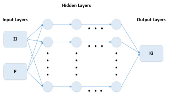
Figure 1.
A Typical feed forward ANN structure.
The output of an ANN of the structure described above is expressed in compact matrix form by
where represents the activating sigmoid function given by
The vectors size in Equation (8) is , , , , , for a system of inputs and outputs and units in the hidden layer. The training procedure needs to provide optimal values for model weights in total.
2.4. Data Compression
Although gas recycling enhances the effect of composition to the prevailing k-values, this effect is still expected to be weak compared to that of pressure and temperature thus implying that the extended fluid composition exhibits high cross correlation over the datasets generated by the sample simulations. Such correlation needs to be removed prior to introducing the composition to the model input to exclude ANN input redundancy, reduce the input vector size and achieve easier and faster training. Similarly, it has been shown that the prevailing k-values live in a space the dimensionality of which depends on the binary interaction coefficients (BICs), and it can be reduced down to only three regardless of the number of components when all BICs are set to zero [54].
Clearly, the application of some dimensionality reduction method is a necessity to simplify the training procedure and it will only slightly affect the trained ANN speed performance as it will be used only to preprocess any future input during the real reservoir simulation. In this work, it was decided to utilize only the simplest, linear compression method, that is principal components analysis [52]. Although this method only accounts for linear relationships between individual inputs, it was shown that in this specific application, the input and output dimensionality can still be greatly reduced. PCA aims at identifying directions in the original data space, known as principal components, on which the data points projections exhibit maximum variance. Every next direction is selected to be orthogonal to the previous ones to ensure a new uncorrelated coordinates system. The fact that the variance percentage captured by each component is maximized leads to their ordering from the most to the less important ones. Therefore, the original data space can be reproduced fairly and accurately by fewer components, thus leading to the formation of a coordinate system of fewer coordinates, hence to dimensionality reduction.
More specifically, let data points , each of size , be treated with the PCA method. The principal components are obtained by considering the mean-centered data points and they are collected in the columns of matrix . The projection of any original datapoint to a subset of components is obtained by
Matrix is and the projection of datapoint of size in the reduced space is of size . The fewer are the components to be retained, i.e., the smaller is , the more is the dimensionality reduction. The optimal number is determined by considering the error between the original and the reconstructed data points , i.e.,
3. Results and Discussion
To demonstrate the value of the proposed method, the EoS model of a real, high yield gas condensate was utilized. The EoS model was used to setup the sample simulations that generate the training dataset. Subsequently, the trained models were evaluated for their accuracy against the training, validation, and testing datasets. To cross-check the trained models performance, each one of the sample simulation models was forced to reproduce the datasets used by the other models which were alien to it. The results are analyzed in a concise, visual manner that proves the value of the proposed ML application.
3.1. Generation of the Training Data
To generate the training dataset, sample simulations were set up to capture the effects of dry gas recycling on k-values in liquid condensation and revaporization. A 10 × 10 × 1 grid block model was selected as a simplistic representation of a gas condensate reservoir with a uniformly distributed porosity in [0.15–0.25] and normally varying permeability around 20 mD, across both the x and y directions [55]. An isothermal reservoir was assumed at 220 °F, and the initial pressure was set at 3000 psia.
The reservoir fluid EoS model consisted of 20 components, and it was deliberately chosen to be rich in heavy components as this is typical of a retrograde gas condensate system. Two components were permanent gases (N2 and CO2), and the ten heaviest components were pseudos. The component properties and composition of the utilized fluid are shown in Table 1. The phase envelope of the reservoir fluid is given in Figure 2, and the liquid dropout curve, showing a maximum condensation level of more than 6%, is illustrated in Figure 3. The fluid’s saturation pressure at reservoir conditions equaled 2950 psia, that is slightly below the initial one (3000 psi).

Table 1.
Component properties and composition of the reservoir gas.
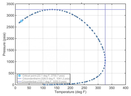
Figure 2.
Phase envelope of the retrograde gas condensate used in the study.
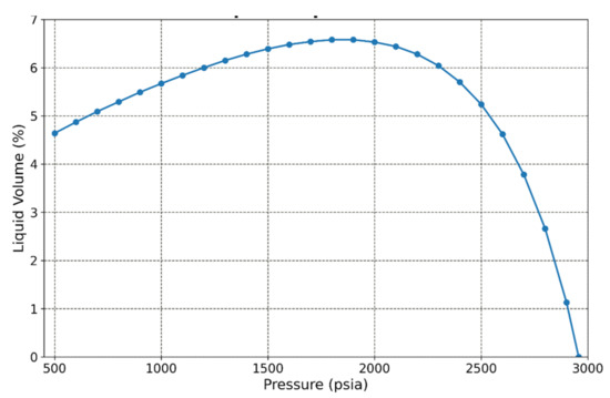
Figure 3.
Liquid dropout curve of the retrograde gas condensate used in the study.
To simulate the gas recycling process, the produced gas during the simulation runs was either flashed directly at standard conditions, where it was separated into reinjection dry gas and liquid condensate, or it was driven at the surface through a more complex series of separators before being flashed at standard conditions. The surface utilization system directly affects the maximum condensate amount produced thus leading to a leaner reinjection gas (stronger gas stripping from its heavier components) when the separator train is used. Five scenarios were setup by utilizing three amounts of gas reinjection and two alternative surface treatment procedures. The first three scenarios considered surface gas to be produced at the surface by direct flash and 80%, 60% and 20% of that gas be reinjected back to the reservoir. Two more scenarios utilized 40% and 80% of the dry gas produced after being treated through a separator train. All scenarios are listed in Table 2.
Table 2.
Sample simulation runs.
As the reservoir gas feed that arrives at the producers keeps changing slowly over time, so does the composition of the reinjected dry gas. To study that effect, the feed composition was monitored throughout the sample simulations, and it was verified that the composition change rate was quite slow. As commercial simulators cannot continuously update the injection gas composition, a five-year reoccurring gas composition update was forced. The produced gas composition of a specific cell in the reservoir model was regarded as representative of the reservoir’s production stream at that time. The cell selected was (3,2) in the 10 × 10 × 1 block reservoir, as shown in Figure 4, as it was located close to a production well (producer 1) and therefore exhibited a composition equivalent to that of the produced fluid without being affected by the pressure drop that the near wellbore region experienced. At the same time, it was close to an injection well (gas injector 1) to allow for the injected gas effect to be pronounced by making its composition leaner.
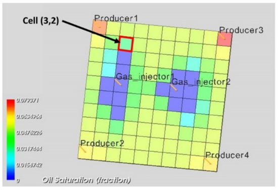
Figure 4.
The 10 × 10 block simplistic gas condensate reservoir. The composition in cell (3,2) was regarded as representative of the average overall reservoir composition.
The dry gas composition collected at the surface was obtained by running regular flash calculations using the reservoir fluid’s EoS model. For the direct flash, the surface conditions were set to the regular values of 14.7 psi and 60 °F. For the separator selected, two separators were set at pressures equal to 500 and 150 psi and at temperatures of 120 °F and 80 °F, respectively. The second separator liquid stream was eventually driven to a tank at standard conditions. Note that for the case of a separator train, the dry gas reinjected is usually the average gas stream from the separators or even by all separators and the tank. Although the averaging needs to be done on a molar basis, a gas-to-oil ratio, GOR, basis can also be used thanks to the ideal gas law that governs the dry gas behavior at the surface and renders volumetric ratios as equal to molar ones. In this work, the gas averaging was performed by considering the gas streams obtained by all separation stages, that is, the two separators and the tank. The separation process is shown in Figure 5. The calculated reinjected dry gas composition at various time instances during the sample simulations is shown in Table 3.
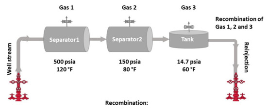
Figure 5.
The produced gas passes through a train of separators before its recombination and reinjection in the reservoir.
Table 3.
Sample simulation reinjected gas composition.
According to scenario 1, only 20% of the produced surface dry gas was reinjected to the reservoir. Four production wells were set to produce at a fixed rate of 7 MMscf/day and two gas injectors to inject dry gas at 2.8 MMscf/day for a 10-year production period. The composition of the initial injection gas and the updated one five years later are given in Table 3, based on the composition of cell (3,2). As expected, the limited amount of reinjected gas could not reverse the condensation; therefore, the produced gas composition and its dry gas version were changing over time (for example, the methane content drops from 70.78% to 69.85%). Due to the limited amount of reinjection gas the reservoir pressure at the end of the production period was 260 psia that, clearly, corresponds to a research rather than a realistic production scenario. The liquid saturation reached a maximum value of 5% before starting to decrease again as a response to the reduction in reservoir pressure and the leaning of the reservoir gas.
In scenario 2, four production wells were producing at a fixed rate of 7 MMscf/day each, and two wells were injecting dry gas at a fixed rate of 8.4 MMscf/day each for a production period of 10 years. Based on the composition of cell (3,2), the injected gas composition was updated after five years of production, as shown in Table 3. The reservoir pressure was constantly declining since the amount of the reinjection gas did not provide sufficient pressure maintenance, and it reached 1500 psia at the end of the production period. The liquid saturation reached a maximum average value of 3.6% followed by a reduction due to revaporization.
Scenario 3 also considered a direct flash of the production to a tank followed by an 80% reinjection of the produced gas. Four production wells and two injectors operated at fixed rates of 7 MMscf/day and 11.2 MMscf/day, respectively. The injection rate was further increased to 12 MMscf/day after five years of production. The reservoir pressure exhibited a constant decline and reached 2300 psia by the end of the production period with the partial pressure maintenance being more pronounced during the second period when the injected gas amount was increased. The liquid saturation reached a maximum average value of 3.8%.
Scenarios 4 and 5 utilized the separator train described above to strip the produced gas from its heavy components. More specifically, scenario 4 considered four production wells operating at a fixed rate of 7 MMscf/day each for a 10-year period and two gas injectors injecting surface dry gas at a fixed rate of 5.6 MMscf/day. The initial reinjection composition was updated once in 5 years, as shown in Table 3. The reservoir pressure exhibited a constant decline and reached almost 700 psia at the end of the production period due to the limited reinjection. The liquid saturation reached a maximum value of about 4.2% before declining to about 3% at the end of production.
Finally, scenario 5 utilized four production wells producing at a fixed rate of 7 MMscf/day each for a period of twenty years. This time, two injector wells were injecting during the first 10 years at a fixed rate of 11.2 MMscf/day, each followed by an increased rate of 12 MMscf/day for the next 10 years. The recycling process provided partial pressure maintenance, thus allowing for the extension of the production period to 20 years. The injection gas composition was revised three times during the production period on a five-year basis by separating each time the composition of cell (3,2). At each update the reinjected gas remained constantly lean thanks to the strong stripping by the surface separators leading to a leaner overall reservoir composition through the recycling process. The liquid saturation exhibited a maximum of about 3.8% which was reduced after five years of production, reaching a value as low as 1.8% in the reservoir, while the reservoir pressure at this stage at the end of production was about 1200 psia.
3.2. Machine Learning Models Development
All five scenarios described above were simulated to generate training datapoints. A single input/output combination was collected at each timestep and at each grid block, thus leading to several thousands of data points per scenario. As each scenario ended up at different average pressure, different number of datapoints were collected in each case. To align the datasets and to allow for a cross-checking (as will be described in Section 3.4), 10,000 datapoints were randomly subsampled from the total population of each sample simulation.
Subsequently, principal component analysis was applied to the compositions in the inputs data set as well as to the k-values in the outputs data sets. As expected, the dimensionality reduction achieved came at the expense of accuracy. To identify the number of principal components (PCs) that need to be retained, the original data was reconstructed by applying the inverse transformation, and the maximum reconstruction error was evaluated according to Equation (11). By reducing the number of composition PCs from 20 to 7 and the number of the k-values PCs from 20 to 5 for the directed dataset, the mean absolute relative reconstruction error fell below 0.1% for the composition and less than 0.0003% for the k-values. Similarly, for the datasets utilizing a separator train, the required number of PCs increased to nine and six, respectively. The mean relative error achieved for all scenarios is shown in Table 4. Clearly, despite its simplicity through its linear treatment of the data, the application of the PCA method led to a major reduction of the input/output pairs size. Note that the input vector consists of the reduced composition and of the prevailing pressure, while temperature is not included as the reservoir is isothermal.
Table 4.
Reconstruction error of the PCA method.
With the length of the input and output vectors fixed, the number of ANN neurons in the hidden layer needs to be investigated to ensure enough flexibility and an accurate training of the model. To minimize the risk of overfitting, each dataset was randomly split into three subsets, namely the training, the validation and the testing ones, corresponding to 75%, 10% and 15% respectively. The error over the training dataset is minimized by varying the model parameters, i.e., , , and , using an unconstrained optimization algorithm (in this case it was the Levenberg-Marquardt one [56]), and the training is terminated by the time the training error reaches a local minimum or when the error of the validation dataset begins to increase significantly, whichever comes first. The testing dataset is used to provide an unbiased evaluation of the model fit after the conventional training is completed. It should be noted that overfitting and poor generalization are almost inapplicable in the present context as the training data is abundant and noiseless.
After exhaustively trying various numbers of hidden neurons for each network, it was found that 20 hidden neurons provided sufficiently accurate training for all networks except for scenario 5 (80S) which required slightly more neurons (23) to capture the more complex phase behavior phenomena. Each training took approximately one minute on a regular computing PC, and each combination was attempted 10 times to investigate the possibility of the ANN getting stuck in a local minimum. In all training attempts, the training was discontinued due to the algorithm trapping to a local error minimum rather than an increase of the validation error.
3.3. Trained Models Performance Evaluation
The ANN-based k-values estimators that were built can be utilized in a two-fold manner. They can be used either to provide direct predictions of the k-values or to introduce them as initial guesses to the conventional flash calculations, replacing Wilson’s equation, to determine the phase molar fraction, phase compositions, component masses and fugacities. In the latter case, the conventional algorithm could converge in no more than one iteration as the ANN output consists a very accurate estimate of the exact k-values.
To evaluate the trained models performance and, therefore, to identify which of the two implementation options needs to be utilized, a loss function was defined. In the present case, the relative error was adopted to describe the deviations of the model prediction from the exact solution of the iterative flash calculation and is described by the following equation:
where and correspond to the estimated and the exact k-value, respectively, of the component of the pair. A similar loss function has been defined for the vapor molar fraction relative error where the value estimate is obtained from Equation (1).
By examining the differential equations governing the flow problem in the porous medium [19,20,21], it can be seen that the k-values are combined to the vapor phase molar fraction to come up with the mass of each component in each phase. In fact, mass appears in the equations through the density of each phase. Therefore, it is reasonable to evaluate the accuracy of the final product of interest, that is, the components mass error rather than other measures commonly used such as the error in the components mole fractions or fugacities. For that purpose, the loss function over the components mass predictions accounts for the components mass error in the liquid phase relative to the total mass in the grid block and it is defined by
Note that thanks to mass conservation, the errors of the gas phase are complementary, and they provide no additional information. The basic statistics of each loss function include the average error (), the standard deviation () and the average absolute error as shown in Table 5. As mentioned above, the performance of the ANNs, which were trained against abundant and noiseless data, was similar to all three data clusters, i.e., training, validation and prediction. For that purpose and to simplify the results, the statistics are shown over the full population utilized per model.
Table 5.
Statistics on the training of the ANN models.
To further investigate the performance of the trained models, the histogram of the relative errors together with their superimposed Gaussian distribution curves are shown in Figure 6, Figure 7 and Figure 8. The vertical axis shows the relative error % of each variable considered (k-values, and liquid phase mass). The dashed green lines correspond to the confidence interval whereas the dashed blue line corresponds to the average absolute relative error . Each figure consists of five plots, one for each trained ANN model. All five plots per figure have been normalized to the same scale to allow for their direct comparison. Finally, the red columns at the top and at the bottom of some plots correspond to the sum of cases which exhibit error beyond the limits of the vertical axis.
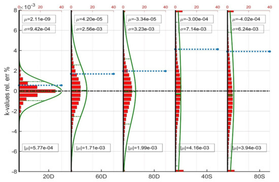
Figure 6.
Average statistics of the prediction of the k-values.
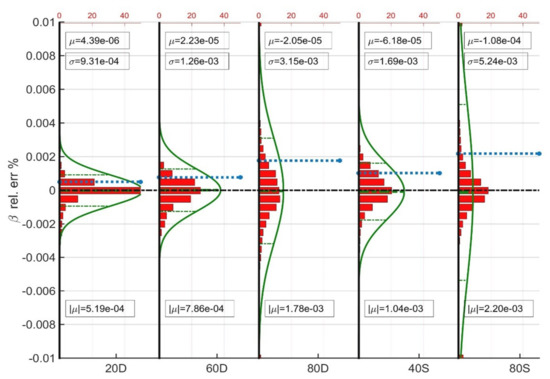
Figure 7.
Average statistics of the prediction of the vapor phase molar fraction ().
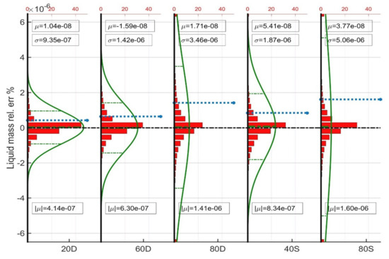
Figure 8.
Average statistics of the prediction of the liquid phase components mass.
From the plots it can be directly seen that all ANNs provide fully balanced predictions as the mean error is almost zero not only for the direct predictions, i.e., the k-values, but also for the vapor phase molar fraction and condensate mass deviations, which all depend on the former. Despite the complexity of the sample scenarios, all ANNs were trained in excellent accuracy as shown by the standard deviation values which indicate perfect predictions for the finally obtained component masses.
Interestingly, all plots verify that the more complex is the gas recycling scenario the wider is the error distribution. Indeed, when switching from the 20D to the 60D and eventually to the 80D, the standard deviation and the average absolute relative error both increase. The error grows even more when considering the separator train-based models as the more stripped recycling gas enhances the variance of the reservoir fluid composition, therefore that of the training data and eventually the complexity of the input-output relationship to be learned by the models. Nevertheless, the liquid mass errors remain negligible, thus guaranteeing accurate calculations during the large-scale reservoir simulation.
The figures in Table 5 and the performance plots clearly indicate that despite their small size, the learning capacity of the ML models suffices to handle the complexity of the relationship between composition, pressure, and temperature on one hand and the prevailing k-values on the other hand. Therefore, the trained models can be safely used during a real reservoir simulation run at practically no cost with the accuracy of the thermodynamic calculations. Even if the ANN predictions would have been used as initial estimates for a conventional, iterative flash algorithm, the latter would not proceed to any iterations as the terminating accuracy would have been achieved by the initial estimates. Note that the number format utilized (A e+XX) corresponds to the exponential form A × 10XX.
3.4. Trained Models Cross-Check
As discussed above, the purpose of the ANNs training is to generate models that can adapt properly to new, previously unseen data. To evaluate that ability, five cross-check sets were setup where a trained ANN was asked to provide predictions against the data utilized to train another model, which is alien to the former. The selected combinations were divided into three galleries according to the ANNs combination, and they are demonstrated in Table 6. The first gallery (D2D) considers pairs of ANNs trained against scenarios that both utilized direct flash of the produced gas at the surface. Gallery 2 (S2S) combines ANNs, both trained against separator train-based data, and gallery 3 (D2S) is the most demanding one as a direct flash ANN is asked to predict the output against which a separator train-based model has been trained. To ensure a fair comparison, each ANNs combination was utilized to predict data that were sharing the same pressure range to avoid extrapolation.
Table 6.
Galleries and ANN combinations in the cross-check exercise.
Similar to the ANN training section, the results of the cross-check are illustrated in Table 7 where the average error (), the standard deviation () and the average absolute error are shown for the vapor phase molar ratio and the liquid phase components mass. Note that this time all results correspond to predictions on brand new data which have never been seen before by the evaluated ANN models.
Table 7.
Statistics on the performance of the ANN models in the cross-check exercise.
When downgrading from the 60D to the 20D, the model is forced to predict the prevailing k-values at compositions lying rather close to the original one due to the limited amount of gas recycling (20% of the surface produced gas rather than 60%). As a result, all predictions are perfectly balanced with the relative error exhibiting a standard deviation of less than 0.003% and the liquid mass relative errors exhibiting an average absolute relative error value of less than 0.000003%. When it comes to the opposite combination, the 60D model is forced to extrapolate toward the compositional space of the 80D sample simulation. In that case, the errors grow bigger, and the standard deviation in the vapor phase molar fraction and liquid phase mass relative errors are found to be equal to 0.01% and 0.00003% (Figure 9). The offset introduced, although very small, does push all relative errors of to negative values (i.e., more gas is produced), thus forcing the liquid phase components mass to positive errors for the vast majority of the data points. Note that both the departing and the arriving model share the same way to bring production to the surface, that is the direct flash to a surface tank.
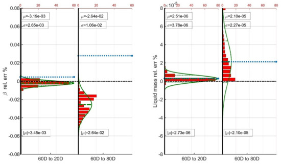
Figure 9.
Average statistics of the D2D gallery ANN combinations.
Sharing the same surface system greatly enhances the prediction capability of the developed models, even when a complex separator train is involved. Indeed, the same stripping process implies similar composition of the recycled gas, hence of the reservoir gas. When switching from the 80S to the 40S model and vice versa, the error distributions are found to be well balanced. Despite the great difference in the amount of recycled gas (80% vs. 40%), the standard deviation of the vapor phase molar fraction error is less than 0.03% while that of the liquid phase components mass is less than 0.00003%, thus rendering the predictions as highly accurate (Figure 10). When the 40S model is extrapolated to predict the performance of the 80D dataset, the errors grow slightly larger with the average absolute relative error increasing from 0.024% to 0.029% and from 0.000018% to 0.000023% for the vapor phase molar fraction and for the liquid mass errors respectively.
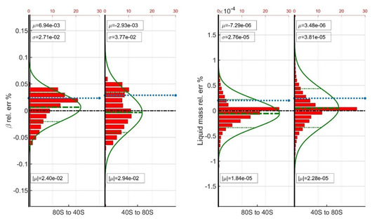
Figure 10.
Average statistics of the S2S gallery ANN combinations.
Forcing a D model to provide predictions on the training dataset of an S model is a complex task as it causes severe extrapolation of the former. The problem becomes even more challenging when the recycling gas amount increases as in the D2S gallery case where a 60D model is forced to provide answers against the training dataset of an 80S one. Results indicate that even in that case the predictions are quite accurate as the vapor phase molar fraction deviation may occasionally be as high as 5% but the average absolute relative deviation equals only 0.6% (Figure 11). The deviation of the liquid phase components mass exhibits significantly low values compared to the previous cross-checks but still exhibits an average absolute relative error value of only 0.0006% which implies that it can be safely used is a regular simulation. Of course, the whole prediction procedure can be safeguarded by a single iteration of the conventional algorithm, in the rare case that this might be needed.
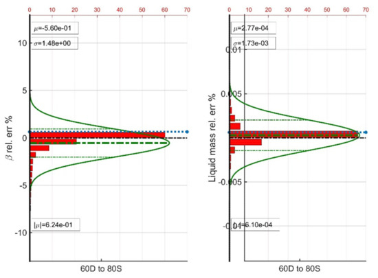
Figure 11.
Average statistics of the D2S gallery ANN combinations.
3.5. Proposed Method Features and Performance
Clearly, the selection of the proper sample simulations plays an important, though not critical, role to the development and the performance of the ML tools to be used in the large-scale reservoir simulation. Bearing in mind that the CPU time required to setup a sample simulation scenario, run it in a regular simulator and train a single ANN against that data is only a few minutes, dozens of sample simulations can be run to build an ANN against a data superset. This way the ANN will have been trained against each possible combination of pressure and reservoir fluid composition and provide very high-quality predictions throughout the simulation of any realistic reservoir simulation. Therefore, unlike other training data generation methods, which might require complex coding, it has been shown that the sample simulations approach can fully serve that task in a simple and elegant manner.
For the CPU time requirements, it was shown that traditional feed forward ANN models of size 8-20-5 can provide all required k-values throughout a regular simulation. Such a network requires two matrix-vector multiplications ( and of size 20 × 8 and 5 × 20 respectively) and 20 exponential function evaluations when implementing the sigmoid function. Additionally, a 7 × 20 matrix needs to be multiplied with the input for the PCA transformation of the data as well as another 20 × 5 one for the back transformation of the predicted output to the k-values space. In fact, the transformation matrices, being just linear transformations, can be embedded to and respectively as a right-hand side and a left-hand side matrix multiplication respectively, thus relieving the need to spend CPU time on them. In addition, the matrix size is expected to become by far smaller when it comes to more realistic EoS models, which usually consist of only 5–10 components.
The calculations described above only account for a very tiny fraction of the time required by a regular flash calculation. It has been shown [39] that such calculations are comparable to the CPU cost to obtain the fugacity of a single-phase trial composition which appears twice in every iteration of the rigorous algorithm, not to mention the cost to set up a Jacobian or a Hessian matrix when a Newton–Raphson or a Newton optimization method are used respectively. Based on the above considerations, it is safe to say that phase behavior calculations, even in their hardest implementation, i.e., in a gas condensate simulation, can be greatly accelerated to stop constituting the bottle neck of compositional reservoir simulation.
4. Conclusions
The need to produce condensate gas fields for meeting the ever-increasing need for the cleanest possible fossil fuel resources has become immense. Gas recycling is necessary to mobilize the trapped liquid condensate and time consuming reservoir simulation is a must in order to optimize the production, but current simulation frameworks are far too time-intensive. To greatly accelerate the simulation CPU time, thus allowing for a more detailed analysis and scheduling of production, ML is proposed. Regression tools are employed to provide direct answers to the k-values prediction issue which, when treated with conventional methods, account for the lion’s share of the total simulation CPU time.
It has been shown that by setting up suitable sample simulations, representative sets of noiseless k-values training data can be obtained which, in turn, are used for the preparation of the ANN-based proxy models. Although the test fluid utilized in this study consisted of 20 components, i.e., it was unusually large, the developed models were shown to exhibit great accuracy, comparable to that of the conventional, rigorous approach, thus rendering machine learning as the appropriate technology to apply to this field.
Author Contributions
Conceptualization, A.S. and V.G.; methodology, A.S. and V.A.; software, V.A.; validation, V.A. and V.G.; resources, V.A.; writing—original draft preparation, V.A. and A.S.; visualization, A.S. All authors have read and agreed to the published version of the manuscript.
Funding
This research received no external funding.
Institutional Review Board Statement
Not applicable.
Informed Consent Statement
Not applicable.
Conflicts of Interest
The authors declare no conflict of interest.
References
- Ashraf, U.; Zhang, H.; Anees, A.; Mangi, H.N.; Ali, M.; Zhang, X.; Imraz, M.; Abbasi, S.S.; Abbas, A.; Ullah, Z.; et al. A core logging, machine learning and geostatistical modeling interactive approach for subsurface imaging of lenticular geobodies in a Clastic Depositional System, SE Pakistan. Nat. Resour. Res. 2021, 30, 2807–2830. [Google Scholar] [CrossRef]
- Townsend, A.F. Natural Gas and the Clean Energy Transition. In EM Compass; International Finance Corporation: Washington, DC, USA, 2019. [Google Scholar]
- Gürsan, C.; Vincent, D.G. The systemic impact of a transition fuel: Does natural gas help or hinder the energy transition? Renew. Sustain. Energy Rev. 2021, 138, 110552. [Google Scholar] [CrossRef]
- Ahmed, T. Equations of State and PVT Analysis Applications for Improved Reservoir Modelling; Gulf Publishing Company: Houston, TX, USA, 2010; ISBN 1-933762-03-9. [Google Scholar]
- Ezekwe, N. Petroleum Reservoir Engineering Practice; Pearson Education: Westford, MA, USA, 2010; ISBN 9780132485210. [Google Scholar]
- Ahmed, T. Reservoir Engineering Handbook, 4th ed.; Elsevier: Amsterdam, The Netherlands, 2010; ISBN 9780080966670. [Google Scholar]
- Craft, B.C.; Terry, R.E.; Rogers, J.B. Applied Petroleum Reservoir Engineering, 3rd ed.; Pearson Education: Westford, MA, USA, 2014; ISBN 978-0133155587. [Google Scholar]
- Jianyi, L.; Ping, G.; Shilun, L. Experimental Evaluation of Condensate Blockage on Condensate Gas Well. Nat. Gas Ind. 2001, 20, 67–69. [Google Scholar]
- Sheng, J.J.; Mody, F.; Griffith, P.J.; Barnes, W.N. Potential to increase condensate oil production by huff-n-puff gas injection in a shale condensate reservoir. J. Nat. Gas Sci. Eng. 2013, 2, 46–51. [Google Scholar] [CrossRef] [Green Version]
- Wang, Z.; Zhu, S.; Zhou, W.; Liu, H.; Hu, Y.; Guo, P.; Du, J.; Ren, J. Experimental research of condensate blockage and mitigating effect of gas injection. Petroleum 2018, 4, 292–299. [Google Scholar] [CrossRef]
- Yong, T.; Zhimin, D.; Lei, S. Research status and progress of removing condensate blockage around well in low-permeability gas condensate reservoir. Nat. Gas Ind. 2007, 27, 88–89. [Google Scholar]
- Muskat, M. Some theoretical aspects of cycling, Part 2. Retrograde condensate about wellbores. Oil Gas J. 1945, 45, 53–60. [Google Scholar]
- Hinchman, S.B.; Barree, R.D. Productivity loss in gas condensate reservoirs. In Proceedings of the SPE Annual Technical Conference and Exhibition, Las Vegas, NV, USA, 22–26 September 1985. [Google Scholar]
- Hameed, M.M. Studying the Effect of Condensate Saturation Bank Development around a Production Well in Siba Field/Yamama Formation. Master’s Thesis, University of Baghdad, Baghdad, Iraq, 2015. [Google Scholar]
- Afidick, D.; Kaczorowski, N.; Bette, S. Production performance of a retrograde gas reservoir: A case study of the Arun Field. In Proceedings of the SPE Asia Pacific Oil and Gas Conference, Melbourne, Australia, 7–10 November 1994. SPE-28749-MS. [Google Scholar]
- Barnum, R.; Brinkman, F.; Richardson, T.W.; Spillette, A.G. Gas condensate reservoir behaviour: Productivity and recovery reduction due to condensation. In Proceedings of the SPE Annual Technical Conference and Exhibition, Dallas, TX, USA, 22–25 October 1995. SPE-30767-MS. [Google Scholar]
- Rahimzadeh, A.; Bazargan, M.; Darvishi, R.; Mohammadi, A.H. Condensate blockage study in gas condensate reservoir. J. Nat. Gas Sci. Eng. 2016, 33, 634–643. [Google Scholar] [CrossRef]
- Silpngarmlers, N.; Ayyalasomayajula, P.S.; Kamath, J. Gas condensate well deliverability: Integrated laboratory-simulation-field study. In Proceedings of the International Petroleum Technology Conference, Doha, Qatar, 21–23 November 2005; ISBN 978-1-55563-991-4. [Google Scholar]
- Cao, H. Development of Techniques for General-Purpose Simulators. Ph.D. Thesis, Stanford University, Stanford, CA, USA, June 2002. [Google Scholar]
- Coats, K.H. An equation of state compositional model. Soc. Petrol. Eng. J. 1980, 20, 363–376. [Google Scholar] [CrossRef]
- Young, L.C.; Stephenson, R.E. A generalized compositional approach for reservoir simulation. Soc. Petrol. Eng. J. 1983, 23, 727–742. [Google Scholar] [CrossRef]
- Wilson, G. A modified Redlich-Kwong EOS, application to general physical data calculations. In Proceedings of the Annual AIChE National Meeting, Cleveland, OH, USA, 4–7 May 1968. [Google Scholar]
- Standing, M.B. A set of equations for computing equilibrium ratios of a crude oil/natural gas system at pressures below 1000 psia. J. Petrol. Technol. 1979, 31, 1193–1195. [Google Scholar] [CrossRef]
- Hoffmann, A.E.; Crump, J.S.; Hocott, R.C. Equilibrium constants for a gas condensate system. Trans. AIME 1953, 198, 1–10. [Google Scholar] [CrossRef]
- Whitson, C.H.; Torp, S.B. Evaluating Constant Volume Depletion Data, SPE Paper 10067. In Proceedings of the SPE 56th Annual Fall Technical Conference, San Antonio, TX, USA, 5–7 October 1981. [Google Scholar]
- Whitson, C.; Brule, M. Phase Behavior, SPE Monograph; Henry, L., Ed.; Doherty Memorial Fund of AIME, Society of Petroleum Engineers: Richardson, TX, USA, 2000. [Google Scholar]
- Katz, D.L.; Hachmuth, K.H. Vaporization equilibrium constants in a crude oil/natural gas system. Ind. Eng. Chem. 1937, 29, 1072. [Google Scholar] [CrossRef]
- Winn, F.W. Hydrocarbon Vapor–Liquid Equilibria, In Simplified Nomographic Presentation. Chem. Eng. Prog. Symp. Ser. 1954, 33, 131–135. [Google Scholar]
- Campbell, J.M. Gas Conditioning and Processing, 4th ed.; Campbell Petroleum Series: New York, NY, USA, 1976; Volume 1. [Google Scholar]
- Lohrenze, J.; Clark, G.; Francis, R. A compositional material balance for combination drive reservoirs. J. Petrol. Technol. 1963, 15, 1233–1238. [Google Scholar] [CrossRef]
- Adegbite, J.O.; Belhaj, H.; Bera, A. Investigations on the relationship among the porosity, permeability and pore throat size of transition zone samples in carbonate reservoirs using multiple regression analysis, artificial neural network and adaptive neuro-fuzzy interface system. Pet. Res. 2021, 6, 321–332. [Google Scholar] [CrossRef]
- Martyushev, D.A.; Ponomareva, I.N.; Zakharov, L.A.; Shadrov, T.A. Application of machine learning for forecasting formation pressure in oil field development. Izv. Tomsk. Politekh. Univ. Inz. Georesursov. 2021, 332, 140–149. [Google Scholar] [CrossRef]
- Hung, V.T.; Kang, K.L. Application of machine learning to predict CO2trapping performance in deep saline aquifers. Energy 2022, 239, 122457. [Google Scholar]
- Ali, M.; Jiang, R.; Ma, H.; Pan, H.; Abbas, K.; Ashraf, U.; Ullah, J. Machine learning—A novel approach of well logs similarity based on synchronization measures to predict shear sonic logs. J. Petrol. Sci. Eng. 2021, 203, 108602. [Google Scholar] [CrossRef]
- Ashraf, U.; Zhang, H.; Anees, A.; Mangi, H.N.; Ali, M.; Ullah, Z.; Zhang, X. Application of unconventional seismic attributes and unsupervised machine learning for the identification of fault and fracture network. Appl. Sci. 2020, 10, 3864. [Google Scholar] [CrossRef]
- Hegeman, P.; Dong, C.; Varotsis, N.; Gaganis, V. Application of artificial neural networks to downhole fluid analysis. SPE Reserv. Eval. Eng. 2009, 12, 8–13. [Google Scholar] [CrossRef]
- Varotsis, N.; Gaganis, V.; Nighswander, J.; Guieze, P. A novel non-iterative method for the prediction of the PVT behavior of reservoir fluids. In Proceedings of the SPE Annual Conference, Houston, TX, USA, 3–6 October 1999; ISBN 978-1-55563-155-0. [Google Scholar]
- Gaganis, V.; Homouz, D.; Maalouf, M.; Khoury, N.; Polycrhonopoulou, K. An Efficient Method to Predict Compressibility Factor of Natural Gas Streams. Energies 2019, 12, 2577. [Google Scholar] [CrossRef] [Green Version]
- Gaganis, V.; Varotsis, N. An integrated approach for rapid phase behavior calculations in compositional modeling. J. Petrol. Sci. Eng. 2014, 118, 74–87. [Google Scholar] [CrossRef]
- Gaganis, V. Rapid phase stability calculations in fluid flow simulation using simple discriminating functions. Comput. Chem. Eng. 2018, 108, 112–127. [Google Scholar] [CrossRef]
- Kashinath, A.; Szulczewski, L.M.; Dogru, H.A. A fast algorithm for calculating isothermal phase behavior using machine learning. Fluid Phase Equilibria 2018, 465, 73–82. [Google Scholar] [CrossRef]
- Zhang, T.; Li, Y.; Li, Y.; Sun, S.; Gao, X. A self-adaptive deep learning algorithm for accelerating multi-component flash calculation. Comput. Method. Appl. M. Eng. 2020, 369, 113207. [Google Scholar] [CrossRef]
- Li, Y.; Zhang, T.; Sun, S. Acceleration of the NVT-flash calculation for multicomponent mixtures using deep neural network models. Ind. Eng. Chem. Res. 2019, 58, 12312–12322. [Google Scholar] [CrossRef] [Green Version]
- Poort, J.; Ramdin, M.; Kranendonk, J.; Vlugt, T. Solving vapor-liquid flash problems using artificial neural networks. Fluid Phase Equilibria 2019, 490, 39–47. [Google Scholar] [CrossRef] [Green Version]
- Wang, K.; Luo, J.; Yizheng, W.; Wu, K.; Li, J.; Chen, Z. Artificial neural network assisted two-phase flash calculations in isothermal and thermal compositional simulations. Fluid Phase Equilibria 2019, 486, 59–79. [Google Scholar] [CrossRef]
- Sheth, S.; Heidari, R.M.; Neylon, K.; Bennett, J.; McKee, F. Acceleration of thermodynamic Computations in fluid flow applications. In Proceedings of the 21st European Symposium on Improved Oil Recovery, Vienna, Austria, 19–22 April 2021; pp. 1–13. [Google Scholar]
- Zhang, T.; Yiteng, L.; Shuyu, S.; Hua, B. Accelerating flash calculations in unconventional reservoirs considering capillary pressure using an optimized deep learning algorithm. J. Petrol. Sci. Eng. 2020, 195, 107886. [Google Scholar] [CrossRef]
- Hernandez Mejia, J.L. Application of Artificial Neural Networks for Rapid Flash Calculations. Master’s Thesis, University of Texas, Austin, TX, USA, August 2019. [Google Scholar]
- Wang, S.; Sobecki, N.; Ding, D.; Zhu, L.; Wu, Y.S. Accelerating and stabilizing the vapor-liquid equilibrium (VLE) calculation in compositional simulation of unconventional reservoirs using deep learning based flash calculation. Fuel 2019, 253, 209–219. [Google Scholar] [CrossRef]
- Gaganis, V.; Marinakis, D.; Samnioti, A. A soft computing method for rapid phase behavior calculations in fluid flow simulations. J. Petrol. Sci. Eng. 2021, 205, 108796. [Google Scholar] [CrossRef]
- Orr, F.M. Theory of Gas Injection Processes, 1st ed.; Holte Tie-Line Publications: Copenhagen, Denmark, 2007. [Google Scholar]
- Bishop, C.M. Pattern Recognition and Machine Learning, 1st ed.; Springer: New York, NY, USA, 2006; ISBN 978-0-387-31073-2. [Google Scholar]
- Bishop, C.M. Neural Networks for Pattern Recognition; Oxford University Press: New York, NY, USA, 1995; ISBN 978-0-19-853864-6. [Google Scholar]
- Michelsen, M.L. Simplified flash calculations for cubic equations of state. Ind. Eng. Chem. Process Des. Dev. 1986, 25, 184–188. [Google Scholar] [CrossRef]
- Fanchi, J.R. Principles of Applied Reservoir Simulation, 3rd ed.; Elsevier: Amsterdam, The Netherlands, 2005; ISBN 9780080460451. [Google Scholar]
- Nocedal, J.; Wright, S. Numerical Optimization, 2nd ed.; Mikosch, T.V., Robinson, S.M., Resnick, S.I., Eds.; Springer: New York, NY, USA, 2006; ISBN 0-387-30303-0. [Google Scholar]
Publisher’s Note: MDPI stays neutral with regard to jurisdictional claims in published maps and institutional affiliations. |
© 2022 by the authors. Licensee MDPI, Basel, Switzerland. This article is an open access article distributed under the terms and conditions of the Creative Commons Attribution (CC BY) license (https://creativecommons.org/licenses/by/4.0/).