Using Self-Organizing Maps to Elucidate Patterns among Variables in Simulated Syngas Combustion

 ,
, 
Abstract
:1. Introduction
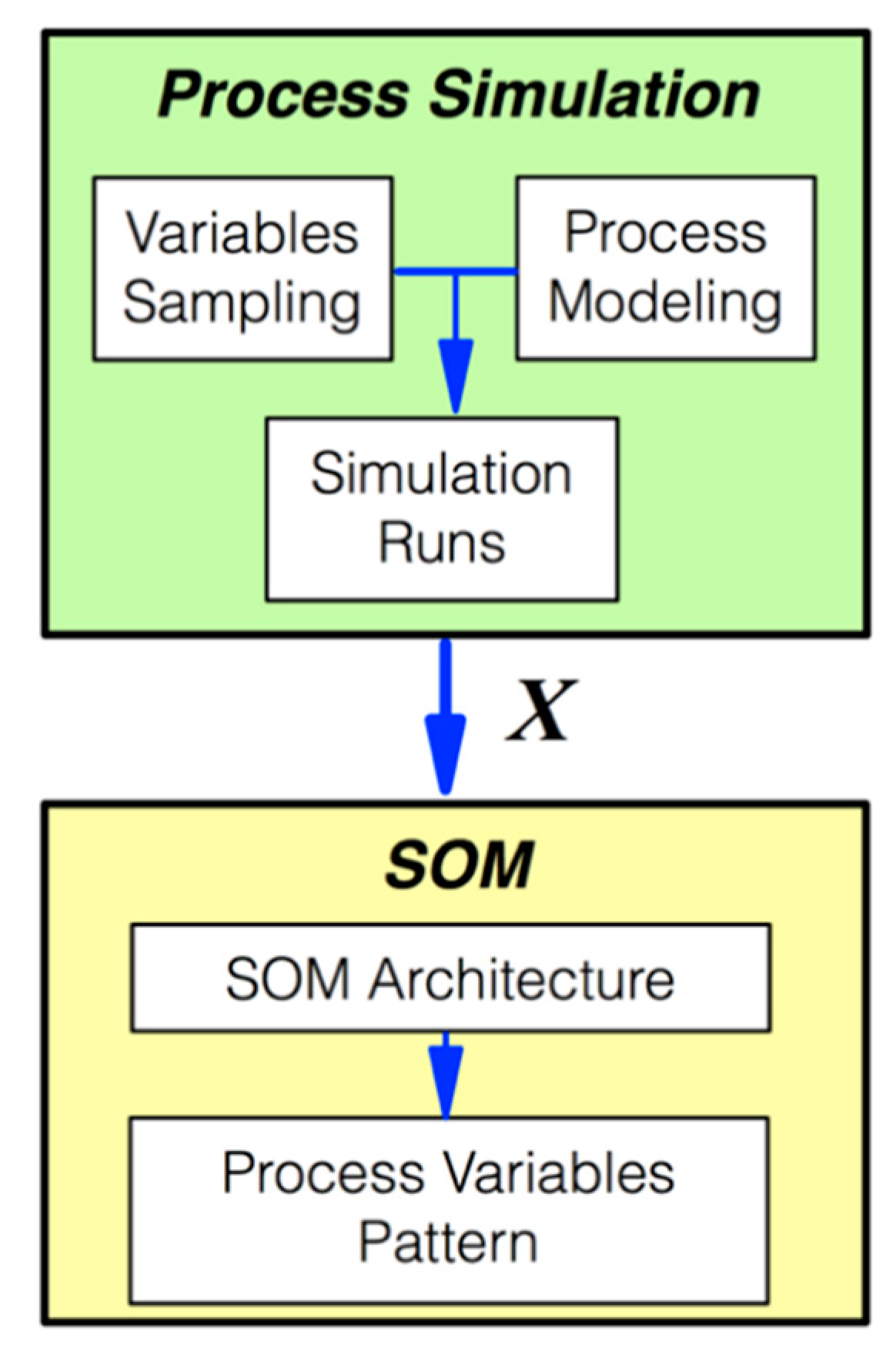
2. Methodology
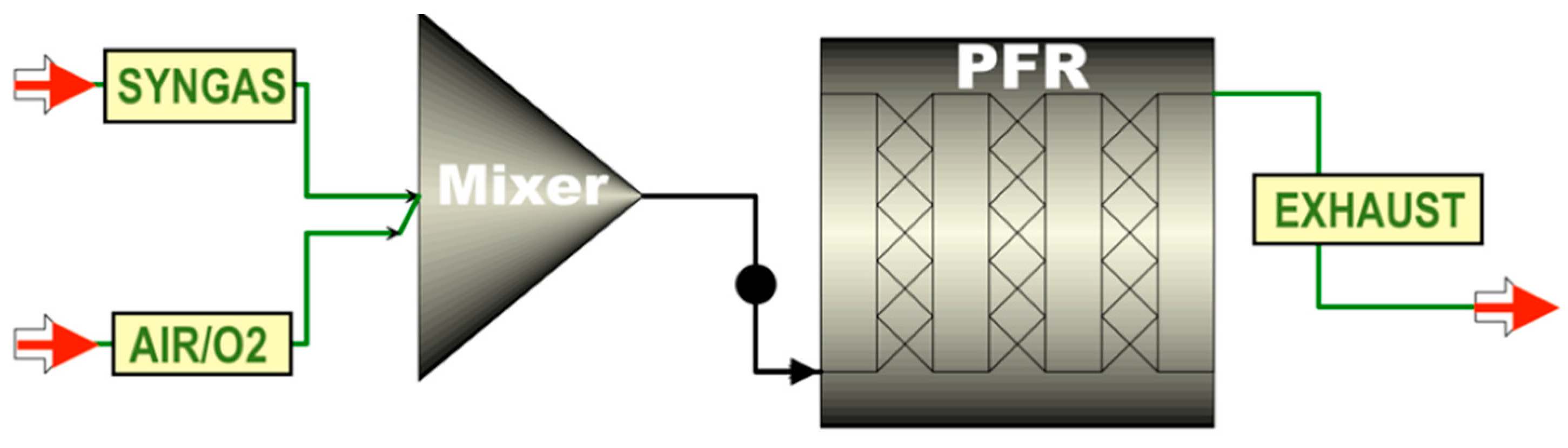
2.1. Process Kinetics Simulation
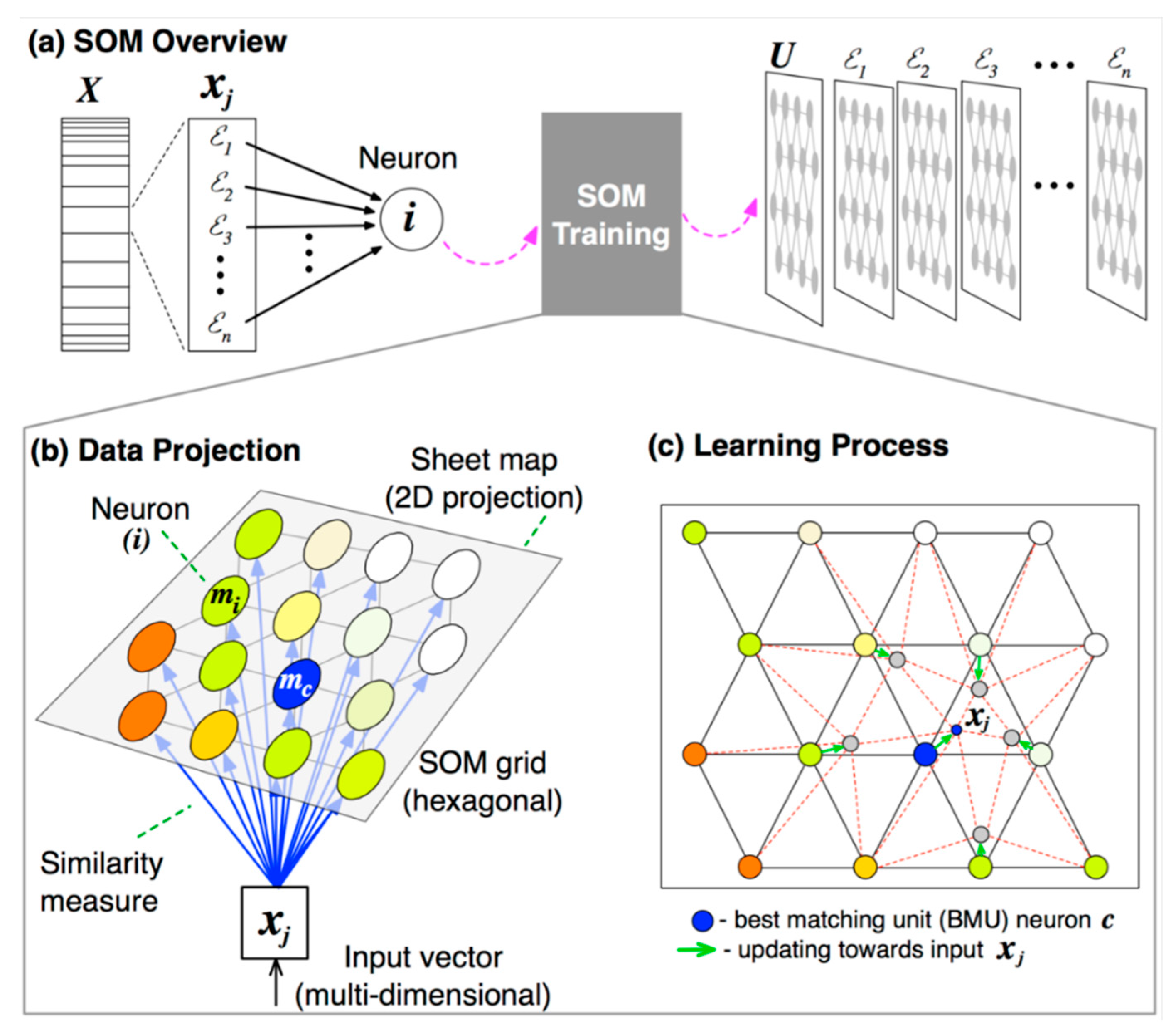
2.2. Variables Pattern Recognition via SOM
2.2.1. Data Pre- and Post-Processing
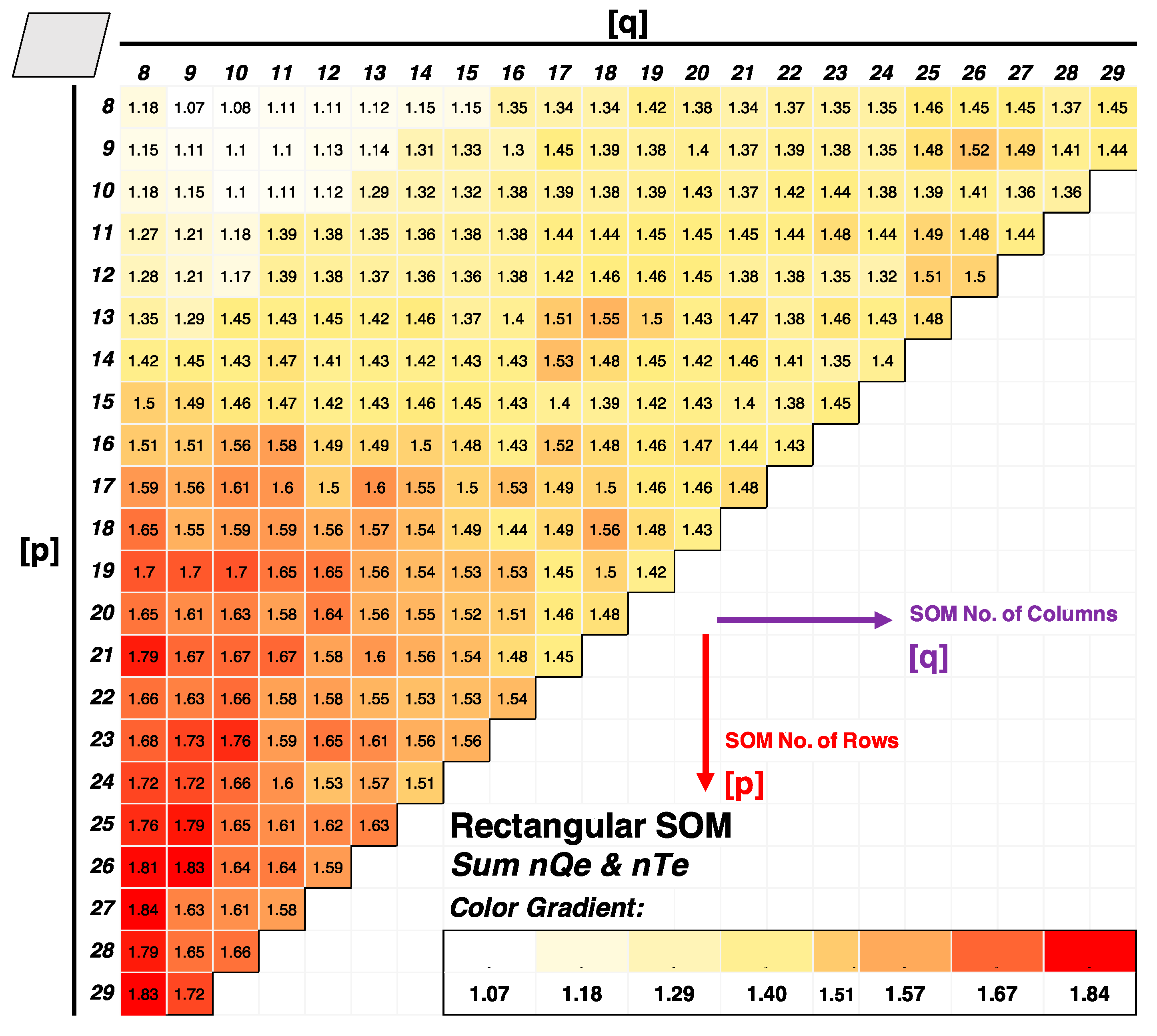
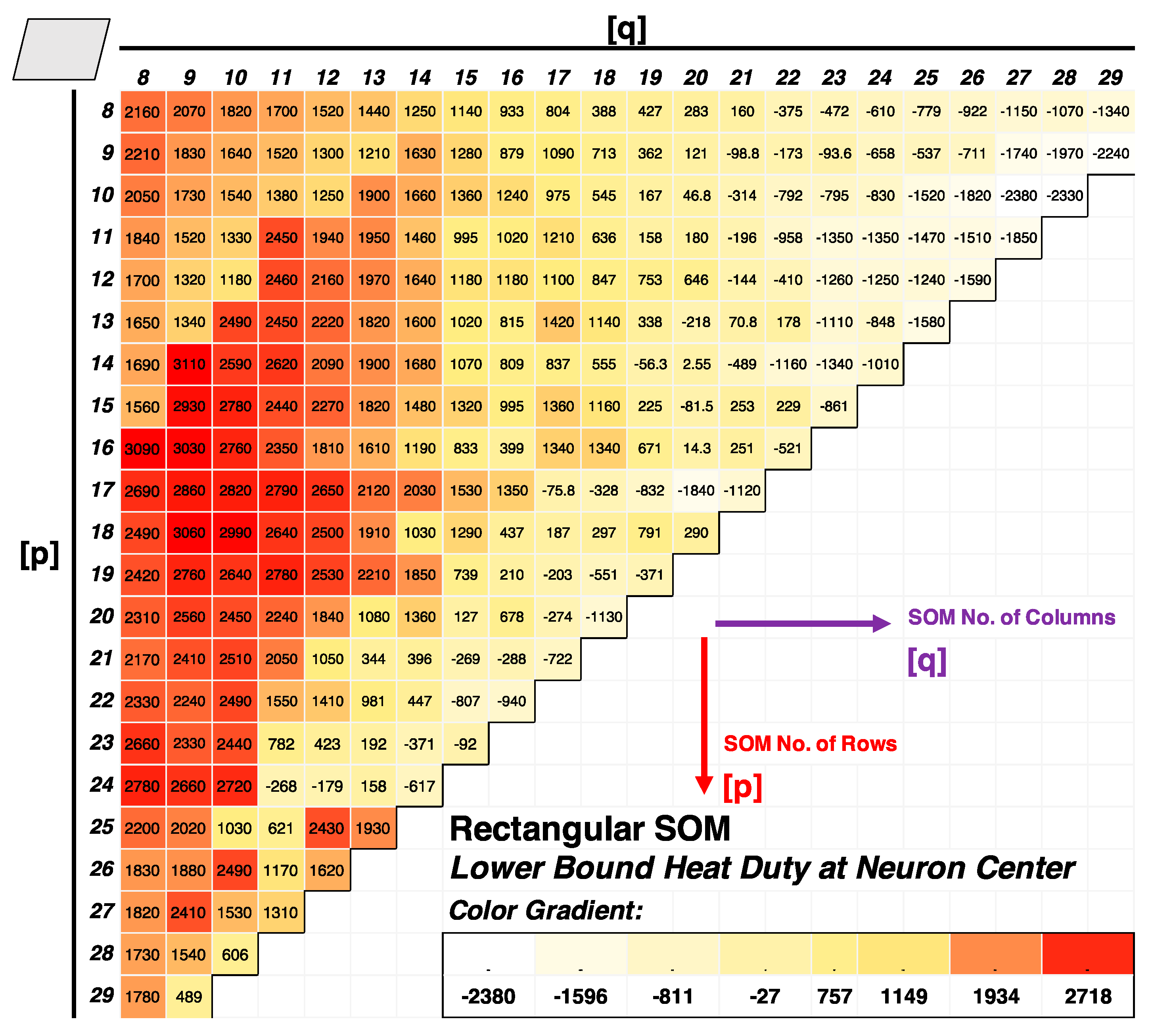
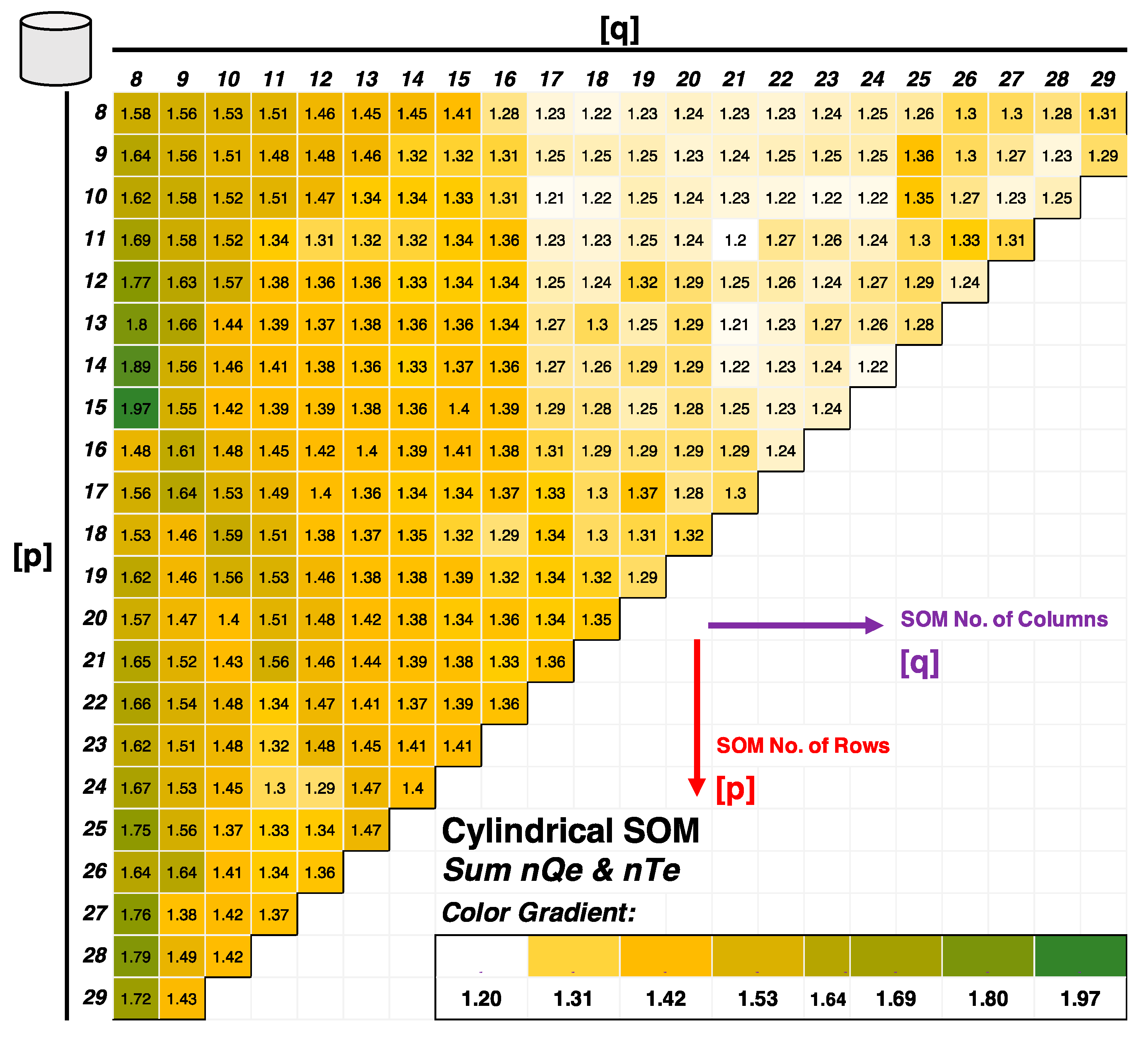
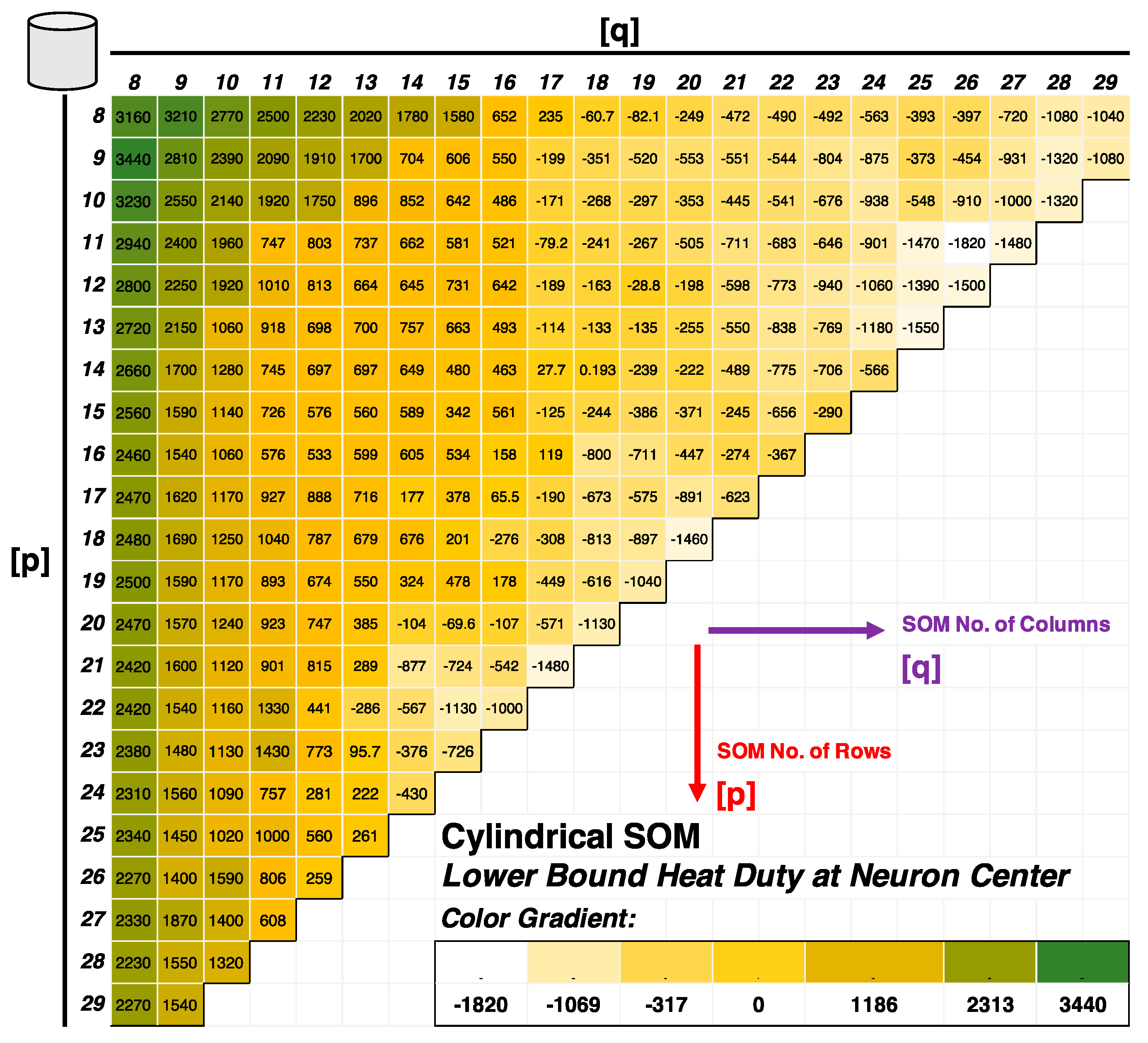
2.2.2. Lattice Structure, Map Shape, and Size
2.2.3. SOM Initialization and Training
3. Results
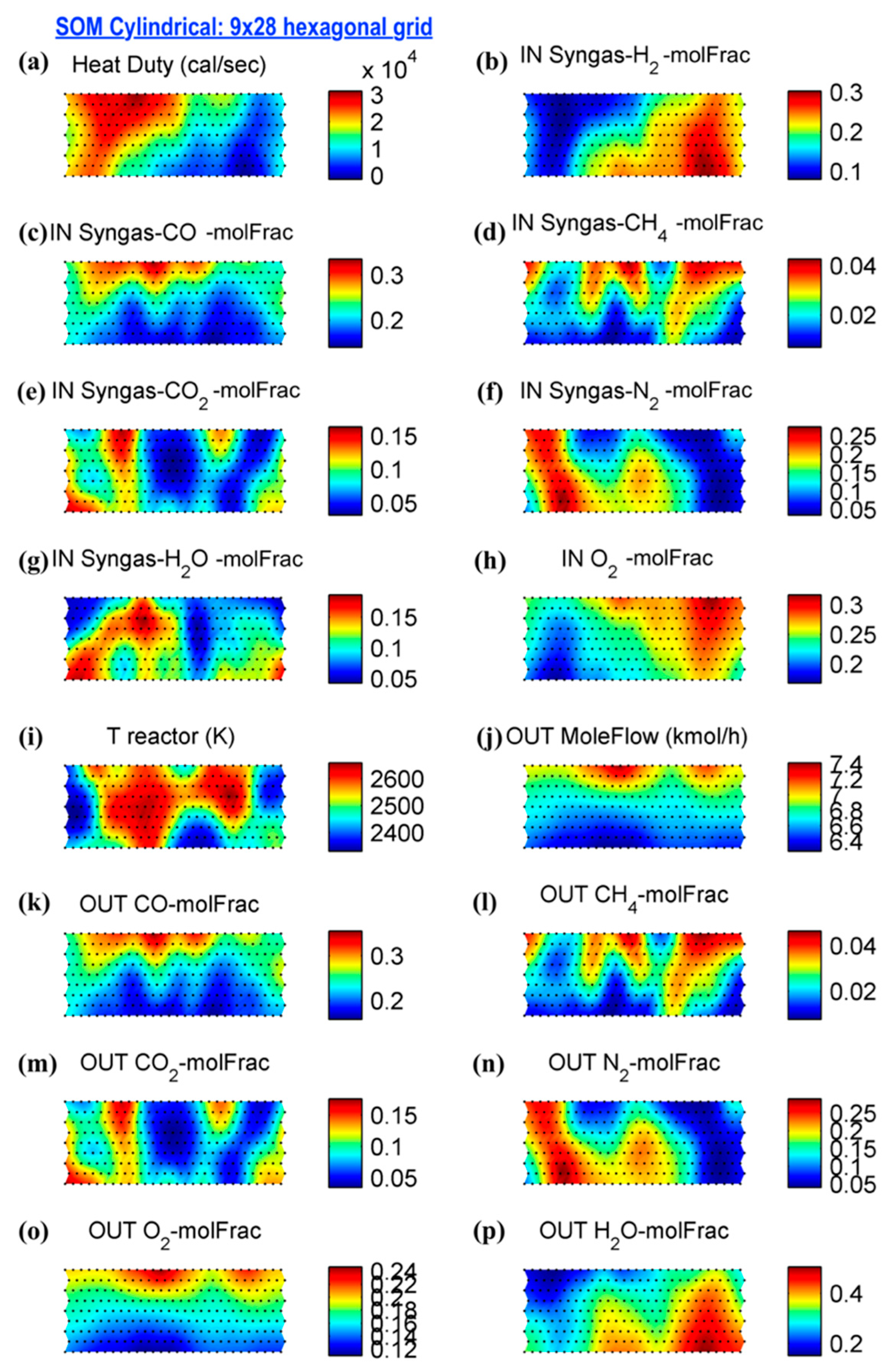
3.1. SOM Architecture
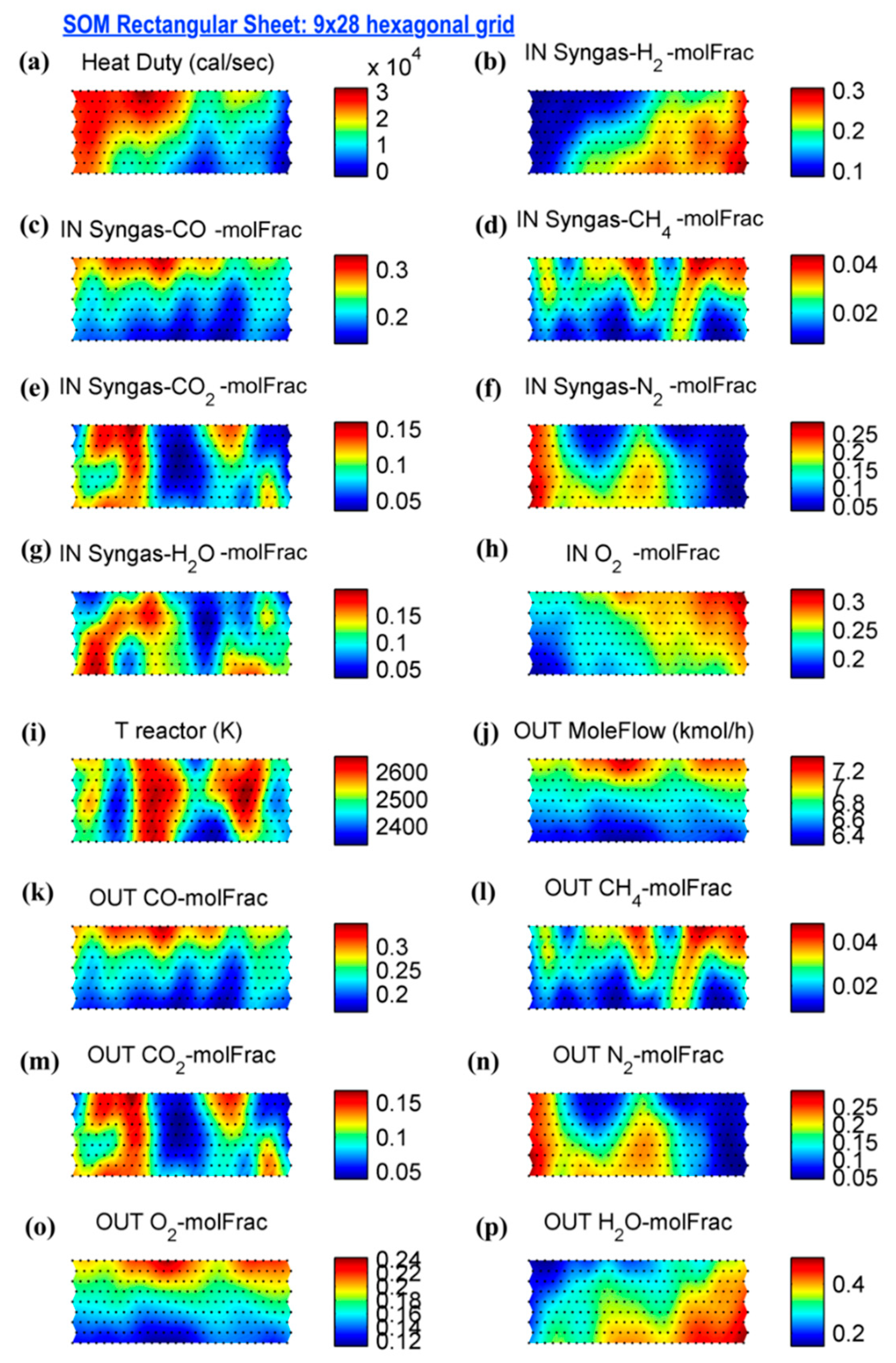
3.2. Syngas Combustion Variables Pattern
4. Discussion
Supplementary Materials
Author Contributions
Funding
Acknowledgments
Conflicts of Interest
Nomenclature
| ANN | artificial neural network |
| chemical species concentration, mol/m3 | |
| rate of generation (+) or consumption (−) of in reaction step , mol/m3/s | |
| reaction constant parameter in reaction | |
| reaction temperature, degree K | |
| gas-phase mole fraction of chemical species at reactor exhaust, % | |
| gas-phase mole fraction of chemical species in the syngas feed, % | |
| BMU | best-matching unit neuron in the SOM grid |
| SOM input dataset of dimension × | |
| th feature variable of the SOM input dataset , | |
| th observation vector in the SOM input dataset , | |
| weight vector of th neuron in the SOM grid | |
| PFR | plug-flow reactor |
| SOM | self-organizing map |
| Te | topographic error of trained SOM |
| Qe | quantization error of trained SOM |
References
- Whitty, K.J.; Zhang, H.R.; Eddings, E.G. Emissions from Syngas Combustion. Combust. Sci. Technol. 2008, 180, 1117–1136. [Google Scholar] [CrossRef]
- Yang, L.; Ge, X. Chapter Three-Biogas and Syngas Upgrading. In Advances in Bioenergy; Li, Y., Ge, X., Eds.; Elsevier: Amsterdam, The Netherlands, 2016; pp. 125–188. [Google Scholar]
- De Kam, M.J.; Morey, R.V.; Tiffany, D.G. Integrating Biomass to Produce Heat and Power at Ethanol Plants. Appl. Eng. Agric. 2009, 25, 227–244. [Google Scholar] [CrossRef] [Green Version]
- Martinez, J.D.; Mahkamov, K.; Andrade, R.V.; Lora, E.E.S. Syngas production in downdraft biomass gasifiers and its application using internal combustion engines. Renew. Energy 2012, 38, 1–9. [Google Scholar] [CrossRef]
- Gupta, A. Introduction to Deep Learning: Part 1. In Chemical Engineering Progress; AIChE: New York, NY, USA, 2018; pp. 22–29. [Google Scholar]
- Dimian, A.C.; Bildea, C.S.; Kiss, A.A. Chapter 2-Introduction in Process Simulation. In Integrated Design and Simulation of Chemical Processes; Dimian, A.C., Bildea, C.S., Kiss, A.A., Eds.; Elsevier: Amsterdam, The Netherlands, 2014; pp. 35–71. [Google Scholar]
- Dimian, A.C.; Bildea, C.S.; Kiss, A.A. Chapter 1-Integrated Process and Product Design. In Integrated Design and Simulation of Chemical Processes; Dimian, A.C., Bildea, C.S., Kiss, A.A., Eds.; Elsevier: Amsterdam, The Netherlands, 2014; pp. 1–33. [Google Scholar]
- Kohonen, T. Self-Organizing Maps, 3rd ed.; Infromation Sciences; Kohonen, T., Ed.; Springer: New York, NY, USA, 2001. [Google Scholar]
- Kohonen, T. Self-Organizing Feature Maps. In Self-Organization and Associative Memory; Springer: New York, NY, USA, 1989. [Google Scholar]
- Kohonen, T. Essentials of the self-organizing map. Neural Netw. 2013, 37, 52–65. [Google Scholar] [CrossRef] [PubMed]
- Lobo, V.J.A.S. Application of Self-Organizing Maps to the Maritime Environment. In Information Fusion and Geographic Information Systems; Springer: Berlin/Heidelberg, Germany, 2009. [Google Scholar]
- Vesanto, J. SOM-based data visualization methods. Intell. Data Anal. 1999, 3, 111–126. [Google Scholar] [CrossRef]
- Kangas, J.; Kohonen, T. Developments and applications of the self-organizing map and related algorithms. Math. Comput. Simul. 1996, 41, 3–12. [Google Scholar] [CrossRef]
- Rumelhart, D.E.; Zipser, D. Feature Discovery by Competitive Learning. Cogn. Sci. 1985, 9, 75–112. [Google Scholar] [CrossRef]
- Faigl, J. An Application of Self-Organizing Map for Multirobot Multigoal Path Planning with Minmax Objective. Comput. Intell. Neurosci. 2016, 2016, 1–15. [Google Scholar] [CrossRef] [PubMed] [Green Version]
- Resta, M. Graph Mining Based SOM: A Tool to Analyze Economic Stability. In Applications of Self-Organizing Maps; Johnsson, M., Ed.; IntechOpen: Rijeka, Croatia, 2012. [Google Scholar]
- Kamimura, R. Social Interaction and Self-Organizing Maps. In Applications of Self-Organizing Maps; Johnsson, M., Ed.; IntechOpen: Rijeka, Croatia, 2012. [Google Scholar]
- Benítez-Pérez, H.; Ortega-Arjona, J.L.; Pérez, A.B. Using Wavelets for Feature Extraction and Self Organizing Maps for Fault Diagnosis of Nonlinear Dynamic Systems. In Applications of Self-Organizing Maps; Johnsson, M., Ed.; IntechOpen: Rijeka, Croatia, 2012. [Google Scholar]
- Henriques, R.; Lobo, V.; Bação, F. Spatial Clustering Using Hierarchical SOM. In Applications of Self-Organizing Maps; Johnsson, M., Ed.; IntechOpen: Rijeka, Croatia, 2012. [Google Scholar]
- Zhang, J.; Fang, H. Using Self-Organizing Maps to Visualize, Filter and Cluster Multidimensional Bio-Omics Data. In Applications of Self-Organizing Maps; Johnsson, M., Ed.; IntechOpen: Rijeka, Croatia, 2012. [Google Scholar]
- Kurdthongmee, W. A Self Organizing Map Based Motion Classifier with an Extension to Fall Detection Problem and Its Implementation on a Smartphone. In Applications of Self-Organizing Maps; Johnsson, M., Ed.; IntechOpen: Rijeka, Croatia, 2012. [Google Scholar]
- Skific, N.; Francis, J. Self-Organizing Maps: A Powerful Tool for the Atmospheric Sciences. In Applications of Self-Organizing Maps; Johnsson, M., Ed.; IntechOpen: Rijeka, Croatia, 2012. [Google Scholar]
- Angeli, S.; Quesney, A.; Gross, L. Image Simplification Using Kohonen Maps: Application to Satellite Data for Cloud Detection and Land Cover Mapping. In Applications of Self-Organizing Maps; Johnsson, M., Ed.; IntechOpen: Rijeka, Croatia, 2012. [Google Scholar]
- Simula, O.; Kangas, J. Process Monitoring and Visualisation Using Self-Organizing Maps. Neural Netw. Chem. Eng. 1995, 6, 371–384. [Google Scholar]
- Liukkonen, M.; Hiltunen, T.; Hälikkä, E.; Hiltunen, Y. Modeling of the fluidized bed combustion process and NOx emissions using self-organizing maps: An application to the diagnosis of process states. Environ. Model. Softw. 2011, 26, 605–614. [Google Scholar] [CrossRef]
- Munoz, I.; Martín-Torre, M.C.; Galán, B.; Viguri, J. Assessment by self-organizing maps of element release from sediments in contact with acidified seawater in laboratory leaching test conditions. Environ. Monit. Assess. 2015, 187, 748. [Google Scholar] [CrossRef] [PubMed] [Green Version]
- Ganhadeiro, T.G.L.; Christo, E.D.S.; Meza, L.A.; Costa, K.A.; Souza, D. Evaluation of Energy Distribution Using Network Data Envelopment Analysis and Kohonen Self Organizing Maps. Energies 2018, 11, 2677. [Google Scholar] [CrossRef] [Green Version]
- Li, M.; Du, W.; Qian, F.; Zhong, W. Total plant performance evaluation based on big data: Visualization analysis of TE process. Chin. J. Chem. Eng. 2018, 26, 1736–1749. [Google Scholar] [CrossRef]
- Arena, U.; Di Gregorio, F. Gasification of a solid recovered fuel in a pilot scale fluidized bed reactor. Fuel 2014, 117, 528–536. [Google Scholar] [CrossRef]
- Khan, A.A.; De Jong, W.; Gort, D.R.; Spliethoff, H. A Fluidized Bed Biomass Combustion Model with Discretized Population Balance. 1. Sensitivity Analysis. Energy Fuels 2007, 21, 2346–2356. [Google Scholar] [CrossRef]
- Campolongo, F.; Cariboni, J.; Saltelli, A.; Schoutens, W. Enhancing the Morris method. In Proceedings of the 4th International Conference on Sensitivity Analysis of Model Output (SAMO 2004), Santa Fe, New Mexico, 8–11 March 2005. [Google Scholar]
- Morris, M.D. Factorial Sampling Plans for Preliminary Computational Experiments. Technometrics 1991, 33, 161–174. [Google Scholar] [CrossRef]
- McDonell, V.G. Key Combustion Issues Associated with Syngas and High-Hydrogen Fuels. 2006. Available online: https://www.netl.doe.gov/research/coal/energy-systems/gasification/gasifipedia/syngas-composition-igcc (accessed on 5 April 2020).
- Vesanto, J.; Himberg, J.; Alhoniemi, E.; Parhankangas, J. SOM Toolbox for MATLAB 5; Helsinki University of Technology: Espoo, Finland, 2000. [Google Scholar]
- Vesanto, J. SOM Implementation in SOM Toolbox. 2005. Available online: http://www.cis.hut.fi/somtoolbox/documentation/somalg.shtml (accessed on 22 October 2019).
- Tian, J.; Azarian, M.H.; Pecht, M. Anomaly Detection Using Self-Organizing Maps-Based K-Nearest Neighbor Algorithm. In European Conference of the Prognostics and Health Management Society; PHM Society: Nantes, France, 2014. [Google Scholar]
- Pölzlbauer, G. Survey and Comparison of Quality Measures for Self-Organizing Maps. In Fifth Workshop on Data Analysis (WDA’04); Elfa Academic Press: Cambridge, MA, USA, 2004. [Google Scholar]
- Vesanto, J. Using SOM in Data Mining. In Epartment of Computer Science and Engineering; Helsinki University of Tehcnology: Espoo, Finland, 2000. [Google Scholar]
- Srinivas, T.; Gupta, A.V.S.S.K.S.; Reddy, B.V. Thermodynamic Equilibrium Model and Exergy Analysis of a Biomass Gasifier. J. Energy Resour. Technol. 2009, 131, 031801. [Google Scholar] [CrossRef]
- Kousheshi, N.; Yari, M.; Paykani, A.; Mehr, A.S.; De La Fuente, G. Effect of Syngas Composition on the Combustion and Emissions Characteristics of a Syngas/Diesel RCCI Engine. Energies 2020, 13, 212. [Google Scholar] [CrossRef] [Green Version]
- Kéromnès, A.; Metcalfe, W.; Heufer, K.A.; Donohoe, N.; Das, A.K.; Sung, C.-J.; Herzler, J.; Naumann, C.; Griebel, P.; Mathieu, O.; et al. An experimental and detailed chemical kinetic modeling study of hydrogen and syngas mixture oxidation at elevated pressures. Combust. Flame 2013, 160, 995–1011. [Google Scholar] [CrossRef] [Green Version]
- Ma, Y.; Weng, J.; Shao, Z.; Chen, X.; Zhu, L.; Zhao, Y. Parallel Computation Method for Solving Large Scale Equation-oriented Models. In Computer Aided Chemical Engineering; Gernaey, K.V., Huusom, J.K., Gani, R., Eds.; Elsevier: Amsterdam, The Netherlands, 2015; pp. 239–244. [Google Scholar]
- Qian, J.; Nguyen, N.P.; Oya, Y.; Kikugawa, G.; Okabe, T.; Huang, Y.; Ohuchi, F.S. Introducing self-organized maps (SOM) as a visualization tool for materials research and education. Results Mater. 2019, 4, 100020. [Google Scholar] [CrossRef]
- Kim, K.P.; Yusof, F.; Daud, Z.B.M. Multi-dimensional reduction using self-organizing map. In 21st National Symposium on Mathematical Sciences (SKSM21); AIP Publishing: Penang, Malaysia, 2014. [Google Scholar]


| Reaction | Rate Expression | Reaction Constant Parameter | |
|---|---|---|---|
| 1 | |||
| 2 | |||
| 3 | |||
| Variables: | (%) | (%) | (%) | (%) | (%) | (%) | (K) |
| Minimum: | 4.65 | 12.03 | 0.00 | 0.84 | 0.11 | 0.05 | 1000 |
| Maximum: | 59.30 | 67.59 | 15.10 | 38.95 | 54.26 | 43.43 | 1500 |
| Median: | 25.55 | 28.02 | 2.93 | 11.24 | 18.10 | 14.62 | 1263 |
| Average: | 24.91 | 28.66 | 2.98 | 11.33 | 17.75 | 14.38 | 1256 |
© 2020 by the authors. Licensee MDPI, Basel, Switzerland. This article is an open access article distributed under the terms and conditions of the Creative Commons Attribution (CC BY) license (http://creativecommons.org/licenses/by/4.0/).
Share and Cite
Fortela, D.L.B.; Crawford, M.; DeLattre, A.; Kowalski, S.; Lissard, M.; Fremin, A.; Sharp, W.; Revellame, E.; Hernandez, R.; Zappi, M. Using Self-Organizing Maps to Elucidate Patterns among Variables in Simulated Syngas Combustion. Clean Technol. 2020, 2, 156-169. https://doi.org/10.3390/cleantechnol2020011
Fortela DLB, Crawford M, DeLattre A, Kowalski S, Lissard M, Fremin A, Sharp W, Revellame E, Hernandez R, Zappi M. Using Self-Organizing Maps to Elucidate Patterns among Variables in Simulated Syngas Combustion. Clean Technologies. 2020; 2(2):156-169. https://doi.org/10.3390/cleantechnol2020011
Chicago/Turabian StyleFortela, Dhan Lord B., Matthew Crawford, Alyssa DeLattre, Spencer Kowalski, Mary Lissard, Ashton Fremin, Wayne Sharp, Emmanuel Revellame, Rafael Hernandez, and Mark Zappi. 2020. "Using Self-Organizing Maps to Elucidate Patterns among Variables in Simulated Syngas Combustion" Clean Technologies 2, no. 2: 156-169. https://doi.org/10.3390/cleantechnol2020011
APA StyleFortela, D. L. B., Crawford, M., DeLattre, A., Kowalski, S., Lissard, M., Fremin, A., Sharp, W., Revellame, E., Hernandez, R., & Zappi, M. (2020). Using Self-Organizing Maps to Elucidate Patterns among Variables in Simulated Syngas Combustion. Clean Technologies, 2(2), 156-169. https://doi.org/10.3390/cleantechnol2020011