Abstract
Estimating soil erodible fraction based on basic soil properties in arid lands is a valuable research topic in the field of soil science and land management. The Proximal Sensing (PS) technique offers a non-destructive and efficient method to assess wind erosion potential in arid regions. By using Partial Least Squares Regression (PLSR) and Support Vector Machine (SVM) models and combining soil texture and chemical properties, determined through Visible-Near Infrared (vis-NIR) spectroscopy in 96 soil samples, this study aims to predict soil erodibility, soil organic matter (SOM), and calcium carbonate equivalent (CaCO3) in arid lands located in Elkobaneyya Valley, Aswan Governorate, Egypt. Results showed that the soil erodibility fraction (EF-Factor) had the highest values and possessed a strong relationship between slope and SOM of 0.01% in determining soil erodibility. The PLSR model performed better than SVM for estimating SOM, CaCO3, and EF-Factor. Furthermore, the results showed that the spectral responses of CaCO3 were observed in separate places in the wavelengths of 570, 649, 802, 1161, 1421, 1854, and 2362 nm, and the wavelengths with SOM parameter were 496, 658, 779, 1089, 1417, 1871, and 2423 nm. The EF-factor shows the highest significant correlation with spectral reflectance values at 526, 688, 744, 1418, 1442, 2292, and 2374 nm. The accuracy and performance of the PLSR model in estimating the EF-Factor using spectral reflectance data and the distribution of data points for both the calibration and validation data-sets indicate a good accuracy of the PLSR model, with RMSE values of 0.0921 and 0.0836 Mg h MJ−1 mm−1, coefficient of determination (R2) values of 0.931 and 0.76, and RPD values of 2.168 and 2.147, respectively.
1. Introduction
Soil is described as a dynamic and heterogeneous system. Its mineral composition is a crucial initial property accounting for soil volume, and thus the understanding of soil system mechanisms and processes requires a multidisciplinary approach and consideration of the various soil factors [1,2]. The soil erodibility fraction (EF-Factor) represents the effect of soil properties and soil profile characteristics on soil loss. It takes into consideration various factors such as soil erodibility, slope length, and slope steepness. This approach can be calculated based on the soil’s texture, organic matter content, and other physical properties that influence its susceptibility to erosion [3]. The EF-Factor assess and determines soil loss worldwide and a strong correlation between EF-Factor and soil loss was proven; therefore, many soil properties including physical and chemical properties affect soil erodibility [4,5,6]. The main limitations of in situ determination of the EF-Factor are the high cost, and time consumption, as well as exhausting work. Therefore, pedo-transfer functions (PTFs) were found to be an easy and rapid alternative for estimating EF-Factor. The PTFs are mathematical relations between major soil characteristics (i.e., texture, organic matter, bulk density, and hydraulic conductivity) which are used to calculate the EF-Factor. These functions are developed based on statistical analysis of field measurements and can provide estimates of the EF-Factor for a particular soil based on its measured properties. PTFs offer a practical and efficient way to estimate the EF-Factor without the need for extensive field measurements. They can be particularly useful in large-scale erosion studies or when detailed soil data are not readily available. However, it is important to note that the accuracy of PTF predictions may vary depending on the specific region and soil conditions. Therefore, validation and calibration of PTFs using local data are crucial to ensure reliable results [7,8]. In the study by [9], the researchers investigated the use of multiple spectra models of soil properties, including wind-stable aggregates, to determine soil erodibility. Soil aggregate stability (AS) indicates how well soil aggregates can withstand disruptive forces such as raindrop impact and runoff. This critical soil characteristic plays a significant role in determining soil loss through water erosion, as it is related to the likelihood of runoff, soil detachment, and transport [10]. Although PTFs are commonly used for EF-Factor estimations, these methods depend on exhausting soil analysis which is costly, time-consuming, destructive, and needs a lot of sample preparation. In case of huge projects, the traditional methods of determining EF-Factor cannot be used except for with limited numbers of soil samples. Therefore, there is a critical need for an advanced, rapid, cheap, and eco-friendly technique for estimating EF-Factor. Thus, visible-near-infrared (Vis-NIR) is the most promising alternative technique for routine soil analysis for total or partial replacement of traditional methods. Vis-NIR spectroscopy involves shining light in the Vis-NIR range onto a soil sample and measuring the reflected or transmitted light. Various soil characteristics, including organic matter content, nutrient levels, pH, and texture, exhibit distinctive absorption patterns in the vis-NIR spectrum [10]. Therefore, vis-NIR has the potential to revolutionize soil testing and monitoring, enabling more efficient soil management practices [11,12]. Spectroscopic methods such as vis-NIR and mid infrared (MIR) spectroscopy, when paired with chemometrics or machine learning techniques, provide a different approach to traditional methods for analyzing soil properties. These techniques are rapid, cost-efficient, and non-invasive, requiring minimal sample preparation and posing no risk of environmental contamination. Furthermore, their portability allows for convenient automated and on-site measurements [13]. Combining proximal soil sensing technologies has been found to improve the precision of soil property predictions compared to using any individual technique [9]. Partial Least Squares Regression (PLSR) was found to be the most commonly used model for estimating soil parameters (i.e., clay, minerals, calcium carbonates, organic carbon, etc.) based on the vis-NIR spectral data. The PLSR is able to correlate spectral variables in the range of (350–2500 nm) with the soil laboratory data, which sorts them in latent components or factors at the same time. Therefore, PLSR is able to extract the complex interactions between spectral variables and soil data [9,11,14,15]. Soil vis-NIR spectroscopy is a rapid, cheap, non-laborious, and eco-friendly technique which does not require preparation of soil samples. Moreover, it can estimate many soil properties simultaneously in the laboratory or in the field [16,17]. The vis-NIR can be used to characterize various soil mineralogical properties such as weathering action [18]. Field spectroscopy reflectance has a high prediction accuracy, using vis-NIR spectral libraries at large scale through various processing methods due to the largely distinctive soil absorption features [19]. Lin et al. (2013) [20] evaluated the potential of vis-NIR spectroscopy for estimating and predicting some soil properties related to soil erosion in Iran using PLSR and SVR with an acceptable R-square for prediction model of soil erosion; the authors mentioned that reflectance spectroscopy coupled with the machine learning algorithm is a promising technique. Wang et al. (2016) [9] used the vis-NIR data for estimating soil erodibility and providing new insights for dynamic determination. Variable selection techniques such as competitive adaptive reweighted sampling-partial least squares (CARS-PLS) have been found to help in selecting the significant spectral variables which affect a specific soil property. Using CARS-PLS in selecting significant spectral bands related to EF-Factor is important because it can help to reduce the number of variables and improve the accuracy of the model. By using CARS-PLS to select the most important spectral bands, it is possible to develop a more accurate and efficient model for predicting EF-Factor, which can then be used to inform land management decisions and improve soil health. Geographic Information Systems (GIS) have been widely used in Egypt for soil characteristics mapping, land evaluation, and land resources identification; furthermore, GIS can assist in land resources identification by analyzing and mapping various natural resources, including soil, water, vegetation, and minerals [5,21]. Remote sensing (RS) is a rapid, cost-effective, and accurate tool for acquiring, analyzing, and classifying data which can be applied for optimal planning of local resources and developing potential productivity strategies [5].
Based on the previous introduction, this study aimed to estimate the EF-Factor using the soil vis-NIR hyperspectral reflectance data; and PLSR and SVM models. Additionally, the study aimed to test the accuracy of spectral models developed by integrating soil texture and some chemical properties in predicting the EF-Factor across different soil units and determine the reliability and accuracy of this approach. This information would be valuable for soil conservation planning, erosion control strategies, and land management decisions.
2. Materials and Methods
2.1. Study Area
The study area is located in Elkobaneyya valley, Aswan Governorate, Egypt between 24°12′18.546″ to 24°19′7.458″ E and 32°45′8.788″ to 32°51′0031.557″ N. It spans an area of approximately 42.34 km2 (Figure 1) and is characterized by its arid climate. The specific location provides a geographic context for understanding the environmental conditions and soil characteristics relevant to the investigation of soil erosion. Based on the USDA Soil Taxonomy [22], the dominant soil orders in the study area are Aridisols and Entisols, characterized by limited rainfall and high evaporation rates, and have minimal development of horizons (distinct layers) due to recent deposition or erosion.
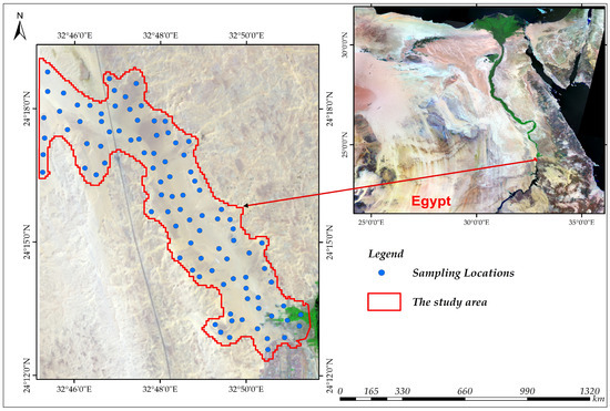
Figure 1.
Geographical location of the study area and soil samples.
Embabi (2018) [23] reported that Nubian sandstones are the most important sedimentary rocks (Quaternary sediments) that cover the study area and are represented by aeolian sands, sand accumulations, and sand sheets. The study area is categorized as under the Hyperthermic soil temperature regime and Torric moisture regime [22]. The desert climatic conditions of the studied site (Table 1) were represented by high temperatures (above 44 °C during summer), while the low average temperatures remain above 18 °C [National Centre for Environmental Information (NOAA), 2023 report; https://www.ncei.noaa.gov/access/monitoring/monthly-report/global/202213, accessed on 19 February 2023]. Moreover, an extremely annual dry climate (precipitation average is 0.12 mm) is observed in the study area with a very low relative humidity (26.17%).

Table 1.
Meteorological data of the study area.
2.2. Sampling Strategy and Laboratory Analyses
To ensure a representative sampling approach, a total of ninety-six soil samples were collected in the study area. These soil samples were geo-referenced using the Global Positioning System (GPS), which provides precise location coordinates for each sampling point (Figure 1). The soil samples were collected using a random sampling approach in February 2022, aiming to achieve the best spatial distribution across the studied area and provide a robust basis for analyzing soil properties and making accurate predictions. After air-drying, the soil samples were ground and sieved to obtain a uniform particle size. The physically described soil samples were assessed based on the Food and Agriculture Organization standard scheme and terminology [24] and Soil Survey Staff [25], then analyzed for some physio-chemical properties. The pipette method was used for determining soil texture as it allows for the determination of the percentage of sand, silt, and clay in the soil sample [26] (Figure 2).
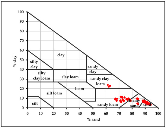
Figure 2.
The CanSIS (Canadian Soil Type Texture Triangle, 1983) textural distribution of the studied soils.
The Walkley–Black method is a widely used technique for the determination of SOM content in soil samples; this method provides a rapid and relatively accurate estimation of SOM content [27]. The determination of calcium carbonate content (CaCO3) content in soil was performed using an acid-base [hydrochloric acid (HCl mol L−1)] titration method. Portable meters were used for on-site measurements of soil EC and pH; these meters provide a convenient and relatively quick way to assess these important soil properties [28].
2.3. The Wind Erodible Fraction (EF-Factor)
EF-factor is a measure of the susceptibility of soil to erosion by wind. It takes into consideration various soil properties that influence wind erosion, such as soil texture, SOM and CaCO3. EF-Factor (Mg h MJ−1 mm−1) was calculated by applying the multiple regression equation proposed by Fryrear et al. (1994) [29], as represented in Equation (1):
where SA, sand content; SI, silt content; CL, clay content.
2.4. Spectral Vis-NIR Measurements Data
The soil samples were first air-dried and then sieved through a 2 mm sieve to remove any large particles. After sieving, the samples were re-dried at a temperature of 30 °C for 10 h. To collect spectral data of the soil samples, a portable spectroradiometer apparatus called FieldSpec 3, manufactured by Analytical Spectral Device (ASD Inc., Cambridge, UK), was used. This device is specifically designed to measure the reflectance or absorbance spectra of various materials, including soil samples. The FieldSpec 3 offers high spectral resolution with an accuracy of 1 nm, meaning it can detect small changes in wavelength. It covers a wide wavelength range from 350 to 2500 nm, allowing for the measurement of a broad spectrum of wavelengths [30]. The 2 mm ground soil samples, with a thickness of 2 cm, were scanned using the FieldSpec 3 device. This scanning process involves shining light onto the soil sample and measuring the amount of light reflected or absorbed at each wavelength. The samples were placed in a container with a diameter of 4 cm and were exposed to natural sunlight to brighten them. White reflectance measurements were taken approximately every 3 min. It is important to note that some bands around 1400 nm (1350 to 1370 nm) and 1900 nm (1820 to 1890 nm) were found to be extremely noisy due to atmospheric effects, so they were removed from the analysis. The collected spectral data can be analyzed to extract information related to various soil properties, such as organic matter content, sand content, silt content, clay content, calcium carbonate content (CaCO3), and other relevant parameters [31]. The high-resolution reflectance data obtained through the software can be further analyzed and interpreted using various techniques, such as spectral indices, spectral matching, or statistical modelling, to extract meaningful information about the soil properties and processes [32]. It is important to ensure accurate calibration of the white reference and proper handling of the instrument to minimize measurement errors and ensure reliable spectral reflectance data [31]. In this study, the recorded soil spectral signatures were converted into a Tab-delimited text file format, which allows for easy import and compatibility with statistical analysis software [32]. When white reflectance was recorded every 5 min, the mean of the 96 recorded spectra was considered. To evaluate the performance and generalization ability of the PLSR model, a 10-fold cross-validation technique was used [33]. The performance metrics used to evaluate the model can include root mean square error (RMSE), coefficient of determination (R2), and correlation coefficients [34] as described in Equations (2)–(4). Figure 3 gives the raw-spectral data of all 96 soil samples.
where Ypred, soil predicted values; Yi, soil measured values mean; Ymeas, soil measured values; n, number of measured or predicted values.
where Y, soil predicted values; X, soil measured values; n, number of measured or predicted values.
where SD is the standard deviation.
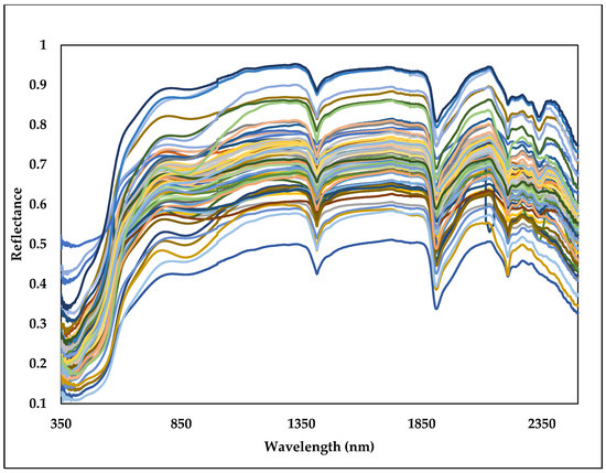
Figure 3.
The raw spectral reflectance data of the soils (n = 96) in different colors in the study area.
2.5. Soil Spectral Data Processing and Analysis
2.5.1. Preparing the Ground: Enhancing Spectral Data for Precise Analysis
To facilitate data processing using Microsoft Excel 2019 software, soil spectral data collected using the ASD spectroradiometer were arranged in a text format using “.csv” files. However, the data was converted to 5 nm intervals using MATLAB R 2019a (ver. 9.60) software. By converting the data to 5 nm intervals, the spectral resolution was reduced, which can help reduce the overall data size and potentially simplify subsequent data analysis to enhance the quality of the calibration and validation models of soil properties [32].
2.5.2. Advanced Statistical Analysis and Innovative Model Development
a. Descriptive statistical analysis: This step involved summarizing and describing the characteristics of a dataset that were used to analyze soil samples, including measures such as mean, standard deviation, minimum and maximum to provide insights into the central tendency, variability, and distribution of the data. Correlation coefficients were also calculated to assess the relationships between different variables within the soil laboratory data and quantify the strength and direction of the linear relationship between two variables. The correlation coefficients can range from −1 to +1. Linear regression analyses were conducted to explore the relationships between predictor variables and a response variable within the soil laboratory data. This model can be used for prediction and estimation of the relationships between variables. IBM® SPSS 22.0 software and Microsoft Excel 2019, used here are both commonly used tools for conducting linear regression analyses [35].
b. Correlation analysis: Using MATLAB R 2019a (ver. 9.60) software, this analysis was performed between each soil property and each 5 nm band reflectance to quantify the strength and direction of the relationship between the two variables. The correlogram generated from the correlation analysis provides a visual representation of the correlation coefficients between the soil properties and the reflectance values at different spectral bands. It helped to identify the best bands that show a strong positive or negative correlation with the soil parameters. These bands can be considered as informative features for predicting or estimating soil properties based on spectral data [35].
c. Models’ development: The soil samples were randomly divided. Two-thirds (2/3) of the 96 soil samples data were chosen to ensure absolutely independent validation and model development calibration. To identify the soil properties values quantitatively, the rest (1/3) of the records were used for model validation. The multivariate regression model (PLSR) was used to develop the prediction models that were used for modelling and predicting relationships between a predictor variables and a response variables data set, as shown in Figure 4 [36].
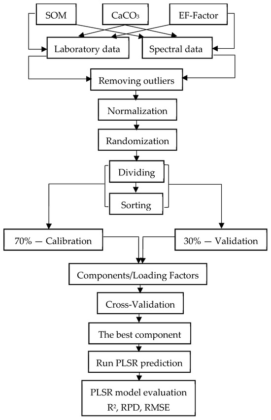
Figure 4.
Model development approach flowchart.
2.5.3. Partial Least-Squares Regression (PLSR) Model
The PLSR model is a multivariate statistical model which is widely utilized for predicting various soil properties based on the vis-NIR spectral data. It selects the best relation between the vis-NIR data (X spectral variables) and soil laboratory data (y laboratory soil parameter) by creating linear orthogonal factors. However, PLSR can deal with complex, heterogeneous, and high dimensional multicollinearity data. The PLSR model equation combines dimensionality reduction with linear regression, as represented in the next Equation (5):
where Y, response variable; T1, T2, T3, …, Tn are the scores obtained through the PLSR analysis; b0, b1, b2, b3, …, bn are the regression coefficients, and ε represents the error term.
Y = b0 + b1 × T1 + b2 × T2 + b3 × T3 + … + bn × Tn + ε
Selection of the Optimal PLSR Calibration Model
To estimate SOM and CaCO3, a technique of (leave-one-out cross-validation) was applied for determining each spectral band’s values of P-coefficients and linking the spectral data with the examined soil parameters. Afterwards, the significant spectral bands which strongly correlated with the examined soil parameters were extracted by the PLSR model [37]. For evaluating the PLSR performance in estimating soil properties and the EF-Factor, some statistical parameters were used. These parameters are root mean square error (RMSE), Ratio of Performance deviation (RPD), and R-squared [38].
PLSR Model (Calibration-Validation Models)
Calibration models were developed by utilizing PLSR in conjunction with leave-one-out (LOO) cross-validation to establish the correlation between soil vis-NIR spectral data (obtained from an ASD spectroradiometer) of the calibration set and the laboratory soil data obtained through traditional soil analysis methods. The spectral and soil laboratory data were merged in the same (.csv file) to be used in R software (version 2022.07.2) for modelling stage. The PLSR model also used the same criterion of calibration to validate the prediction model. However, the outputs of this stage were put in an MS Excel sheet and again exported to R software for conducting model output averaging (MOA) using the predictors’ weighting method, as described in the following Equation (6):
where Yi is the combined outcome at point i from k number of ensemble outcomes, Xik is the realization from the kth contributor model, and Wk is the weighting attributed to that model outcome [39].
Several research studies, i.e., Diks and Vrugt (2010) [40] and Malone et al. (2014) [41]), have employed different MOA methods such as equal weights/simple averaging (SA); ordinary least squares regression averaging (OLS); Bates–Granger averaging (BG), which involves variance-weighted averaging; and Bayesian model averaging (BMA).
The SA applies equal weights to the obtained data from PLSR; while in OLS, regression is used for determining weights for model predictors [42]. Regarding the BG method, variances’ values are used in the models [43], while the BMA assigns weights by considering the uncertainty of each model. However, the higher the likelihood of the method, the higher the prediction accuracy. Further insights into the BMA can be found in Hoeting et al. (1999) [44].
PLSR calibration and validation prediction models were evaluated against their performance and accuracy R2, RMSE, and RPD [45]. In this study, we used the same criterion as Viscarra Rossel et al. (2006) [46], who proposed RPD categories used for prediction model evaluation of RPD > 2.5 (excellent), between 2.0 and 2.5 (very good), between 1.8 and 2 (good), between 1.4 and 1.8 (fair), between 1.0 and 1.4 (poor), and RPD < 1.0 (very poor).
Data Transformation Methods
- Box–Cox transformation
To assess the relationship between the compression indices, a simple regression analysis was carried out after appropriately transforming the variables to meet the normality assumption required for regression analysis. The statistical test revealed that the compression index values did not adhere to a normal distribution but exhibited a skewed distribution. When the relationship between the independent and dependent variables is nonlinear or the dependent variable does not follow a normal distribution, it is essential to transform the variables to approximate a normal distribution before conducting regression analysis.
The Box–Cox transformation is a technique employed to normalize a dependent variable to meet the normality assumption, which is crucial in regression models. If the normality assumption is violated, the validity of the suggested regression model is compromised. To address this statistical requirement, Box and Cox (1964) [47] proposed transforming the dependent variable to eliminate noise, particularly outliers in the data, as described in Equation (7).
where X represents the original data, Y is the transformed data, and the value of λ denotes the transformed data; the value of λ can be determined through maximum likelihood estimation [48]. Specifically, when λ takes on values of 0, 1/2, and −1, the Box–Cox transformation equation corresponds to the logarithmic transformation, square root transformation, and reciprocal transformation, respectively.
2.5.4. Support Vector Machine (SVM) Model
SVM model is a nonlinear model which is commonly used in chemo-metrics, like soil spectroscopy [48], while the standard model is used for a linear classification. This model has low performance in predicting soil parameters compared to the linear regression models. This low accuracy occurs due to the nonlinear regression problems as well as the complexity and heterogeneity of the soil and spectral variables. However, for decreasing this problem, a kernel function [49,50] such as kernel radial basis function (RBF) was found to be a good assistant for enhancing the nonlinear regression relations (Equation (8)).
De Brabanter et al. [51] mentioned that the gamma (ɣ) parameter plays an important role in regulating and balancing the trade-off between smoothness and decreasing the error in calibration model. Moreover, the σ2, which is called (squared bandwidth) as described in (Equation (9)), is required for fine-tuning the RBF kernel algorithm. The initial random parameters are selected using leave-one-out cross validation [52] and subsequently optimized using the conventional simplex technique [53].
where, is a kernel radial basis function, and are vector points in any fixed dimensional space, and σ2 is the squared bandwidth of the Gaussian curve.
ɣ = 1/2 σ2
The vis-NIR features that are produced from the latent variables (LVs) calculated from the PLS regression model serve as the input parameters for training the LS-SVM. Similar methods were employed by Mouazen et al. [54], but instead of using SVM as in the current study, they used a back propagation artificial neural network (BPNN) using the latent variables derived from PLSR as input.
2.5.5. Variables Selection Methods
The Competitive Adaptive Reweighted Sampling (CARS) algorithm, inspired by Darwin’s principle of “the survival of the fittest”, is employed for variable selection in vis-NIR hyperspectral datasets relevant to soil chemometrics. The primary objective of this technique is to identify the best set of wavelengths from the entire spectrum to construct a calibration model with superior performance. The significance of each variable is assessed based on the stability index within the CARS algorithm. This index is defined by Equation (10):
The CARS algorithm consists of the following four steps [55]:
- (i)
- Monte Carlo approach: In this initial step, 80% of the samples from the calibration set are randomly selected;
- (ii)
- Exponentially decreasing function (EDF): In this stage, less significant variables are systematically eliminated. The proportion of variables to be retained is determined using the EDF formula presented in Equation (11):
- (i)
- Adaptive reweighted sampling (ARS): Following the initial elimination based on the EDF, ARS is applied to further remove variables in a competitive manner. ARS operates on the principle of ‘survival of the fittest’ inspired by Darwin’s theory of natural selection. Variables with weights exceeding a specified threshold are retained;
- (ii)
- Assessment of RMSE values: The n subsets generated are evaluated based on their respective RMSE values. The subset that yields the lowest error is selected as the preferred choice.
2.6. Mapping of the Spatial Variability Distribution of Soil Properties
An ordinary kriging interpolation method was used for generating spatial variability maps of the soil properties (SOM, CaCO3, clay, silt, and sand) over the study area. For achieving that, geo-coordinates of the sampling locations and the shapefile (border of the study area) were entered to the geostatistical wizard environment, and then the kriging method was applied. The developed maps were annotated and documented, wherein all mapping requirement (north arrow, legend, scale, etc.) were incorporated.
3. Results
3.1. Description of Soil Properties
The obtained data in Table 2 revealed that soil samples were alkaline where pH values reached 7.97. Low soil content of CaCO3 was observed, where the mean value was 1.60%, while the soil EC varied between 0.22 and 2.65 mS cm−1 (mean = 0.70 mS cm−1). The SOM ranged from 0.04% to 0.50%, while the mean value was 0.22%. Regarding the soil fractions, the minimum and maximum values of clay were 3.08% and 11.59%, respectively, while the sand varied between 66.95% and 94.26%; silt differed from 2.11% to 24.67%, Figure 5. In terms of variability, CaCO3 had the highest coefficient of variation (CV) value of 119.620, silt had the second highest CV value of 77.63%, while sand and pH had the lowest CV values of 9.86 and 4.64, respectively.

Table 2.
Descriptive statistics of soil properties (n = 96).
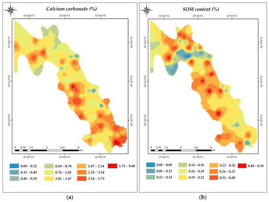
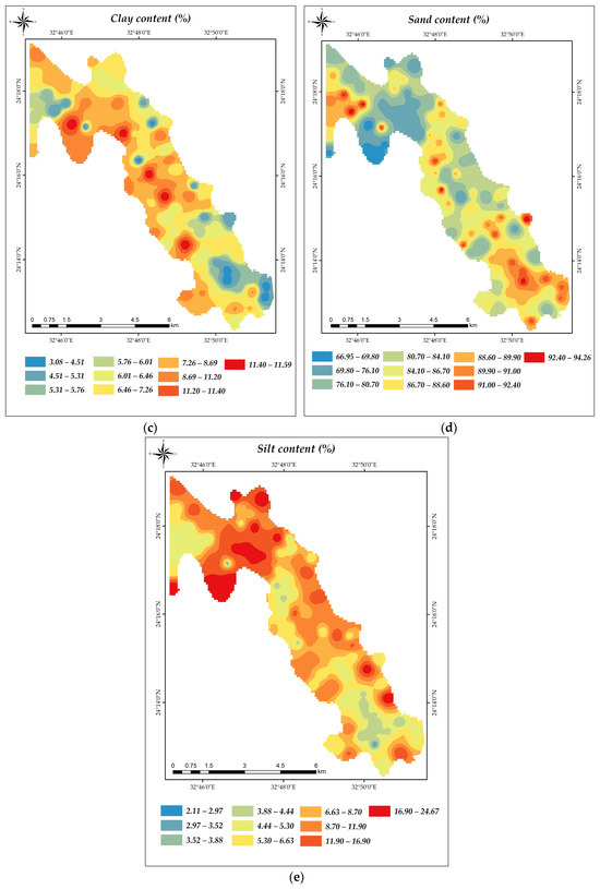
Figure 5.
Data description of the basic soil properties: (a) CaCO3, (b) SOM, (c) clay, (d) sand and (e) silt content %.
3.2. Wind-Erodible Fraction (EF-Factor) Calculation Using the Fryrear Equation
Based on the Fryrear equation [29], the calculated EF-Factor ranged from 0.46 to 0.68, with a mean value of 0.59. The mean EF-Factor in slope lands was significantly higher (0.59) compared to other landforms, which provides an overall representation of the erosion potential within the soil samples, as shown in Table 2 and Figure 6.
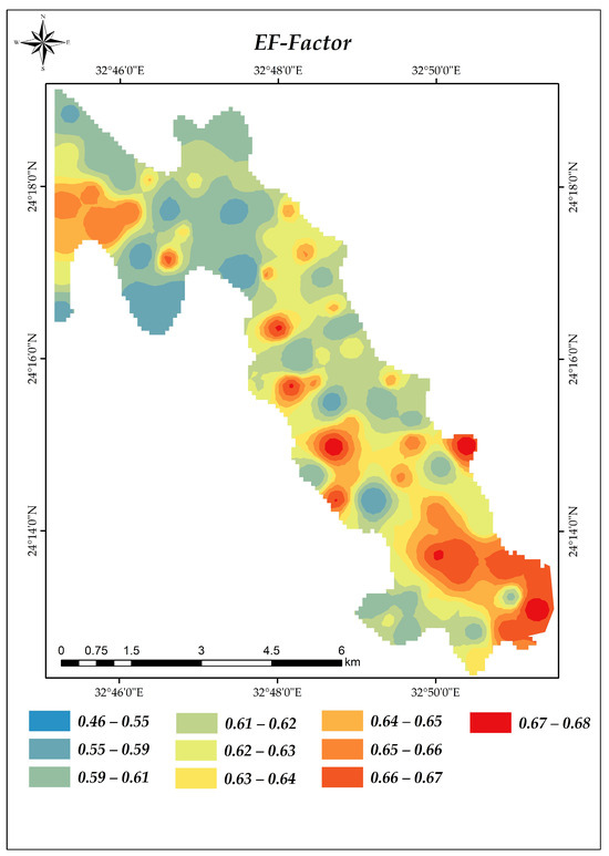
Figure 6.
Wind-erodible fraction (EF-Factor).
3.3. Correlation between Soil Properties and EF-Factor
Based on the correlation analysis, the EF-Factor shows different levels of association with various soil properties (Table 2 and Table 3); SOM showed the highest positive correlation with the EF-Factor, with a correlation coefficient of 0.814 (p < 0.01), indicating that the EF-Factor tends to increase. Additionally, a positive significant correlation was observed between the EF-Factor and CaCO3, with a correlation coefficient of 0.780. Furthermore, a positive but weaker correlation was found between the EF-Factor and soil particles (sand and clay content), with a correlation coefficient of 0.541 and 0.423, respectively.

Table 3.
Pearson’s correlation coefficient (r) between EF-Factor and some basic soil properties.
3.4. Soil Spectra Analysis
Based on Figure 7, which illustrates the Box–Cox plots of the soil features after removing outliers, the Box–Cox transformation is a statistical technique used to normalize data and improve model accuracy by removing redundant or noninformative predictors. By normalizing the data using the Box–Cox transformation, the model can effectively handle any skewness or nonlinearity in the predictors. This normalization process ensures that the predictors are in a suitable format for analysis, leading to improved accuracy in the prediction model. Utilizing the CARS technique in this scenario can enhance the precision of the prediction model by eliminating unnecessary or duplicated predictors from the analysis.
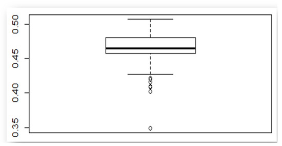
Figure 7.
Box–Cox plots of removing outliers of soil samples (n = 96; removed outliers = 7; n after removing outliers = 89).
According to Figure 8, which demonstrates the variations in spectral reflectance for three soil textural classes with similar SOM content and pH but different clay percentages, there is a distinct shoulder observed in the spectral data between 450 and 700 nm. Additionally, there are three explicit peaks observed at 1380, 1925, and 2124 nm; these spectral features can provide valuable information about the soil composition and properties. Furthermore, specific absorption features are observed around 850 and 2350 nm; these absorption features can be indicative of certain soil constituents or characteristics. Moreover, near 950 nm and between 2350 and 2400 nm, there are also absorption features present in the spectral data; these features can be useful for identifying specific susceptibility of soil to erosion by wind according to soil properties or substances [18].
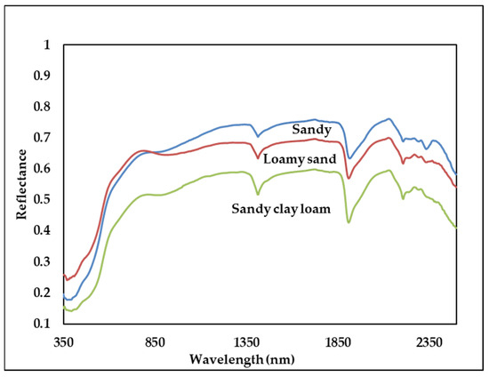
Figure 8.
Changes in spectral reflectance for different soil textural classes.
3.5. Correlation between Spectral Reflectance and EF-Factor
To identify the most significantly correlated bands with each soil parameter (SOM and CaCO3) for estimating the EF-Factor using spectral reflectance data, the correlation coefficient (r) was used to identify the most significant bands and develop point STF for EF-factor prediction with the spectral reflectance in range of 350 to 2500 nm, as shown in Table 4.

Table 4.
The most significantly correlated bands with each soil parameters and EF-factor.
Based on the results, the spectral responses of soil calcium carbonate (CaCO3) were observed at different wavelengths as follows: 570, 649, 802, 1161, 1421, 1854, and 2362 nm, respectively. The correlation coefficient values associated with these wavelengths provide information about the strength and direction of the relationship between the spectral response and the CaCO3 content in the soil. The correlation coefficients for these wavelengths are as follows: −0.1850, −0.1700, −0.0975, 0.0459, 0.0679, 0.0946, and 0.1070, respectively. The highest values of the regression coefficients, which indicate the importance of each wavelength in predicting the CaCO3 content, were observed in the near-infrared (NIR) spectral range, specifically at wavelengths ranging from 2325 to 2365 nm, with a peak at 2340 nm, Figure 9 shows a few other prominent absorption peaks between 2200 and 2300 nm and around 2440 nm.
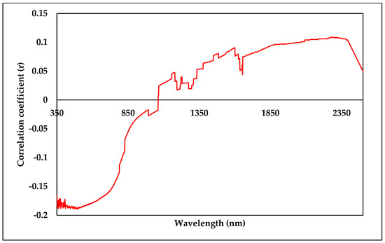
Figure 9.
Correlation coefficient (r) between spectral reflectance values across the Vis-NIR range and CaCO3 content.
The maximum correlation coefficient values for the SOM parameter was observed at different wavelengths, as follows: 496, 658, 779, 1089, 1417, 1871, and 2423 nm, respectively, and the correlation coefficient values for these wavelengths are as follows: 0.0181, 0.0196, 0.0281, −0.0540, −0.0801, −0.1130, and −0.1210, respectively. These correlation coefficient values suggest that there is a weak positive correlation between the spectral response at wavelengths of 496, 658, and 779 nm, and the SOM content in the soil. On the other hand, there is a weak negative correlation between the spectral response at wavelengths of 1089, 1417, 1871, and 2423 nm and the SOM content in the soil, as shown in Figure 10.
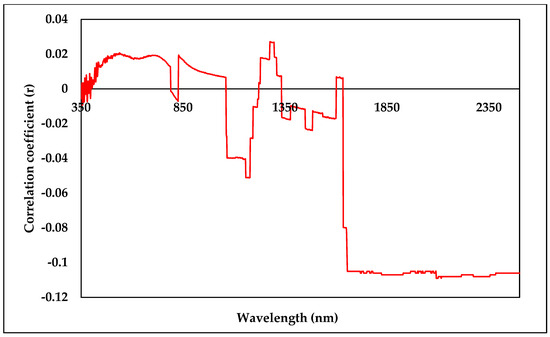
Figure 10.
Correlation coefficient (r) between spectral reflectance values across the Vis-NIR range and SOM.
Correlation coefficient (r) between spectral reflectance values across the Vis-NIR range and EF-Factor was shown in Figure 11. The highest correlation coefficient values were (0.0151 at wavelength of 526, 0.0176 at 688, 0.0356 at 744, −0.0457 at 1418, −0.0758 at 1442, −0.0212 at 2292, and −0.5270 at 2374 nm).
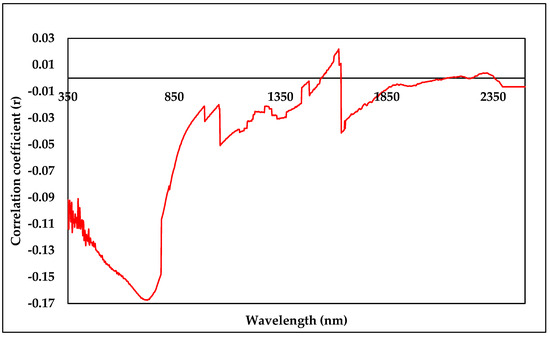
Figure 11.
Correlation coefficient (r) between spectral reflectance values across the Vis-NIR range and EF-Factor.
3.6. Model Development
3.6.1. Prediction of SOM and CaCO3 Using PLSR Model
The obtained data of remaining samples’ number of SOM and CaCO3 after outliers’ removal in each calibration and validation datasets are demonstrated in Table 5. RMSE, RPD, and R2 are also presented.

Table 5.
The predictability assessment of the soil parameters using PLSR and SVM models.
A total of 70% of the SOM datasets (spectral and laboratory) were used in the PLSR calibration model, where the R2, RPD, and RMSE values were 0.71, 2.19, and 0.071%, respectively. The rest of the data (30%) were used in validation model, where the R2, RPD, and RMSE values were 0.58, 2.14, and 0.068%, respectively, as shown in Figure 12.
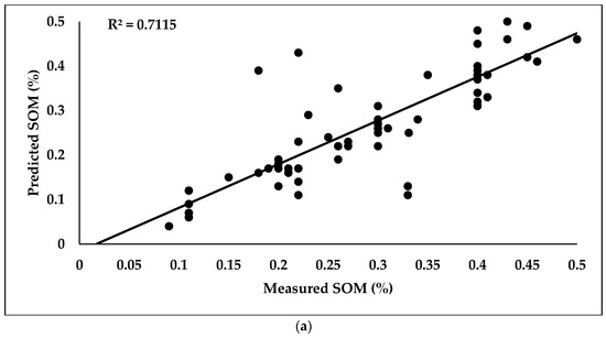
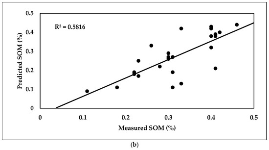
Figure 12.
Scatter plots of predicted (a) and measured (b) SOM content using the PLSR model.
The obtained results (Figure 13) revealed that the R2 of the calibration model of estimating soil CaCO3 was 0.59, while RPD and RMSE values were 2.562 and 0.0982%, respectively. Values of RMSE, RPD, and R2 in the validation model were 0.4163%, 1.936, and 0.51, respectively.
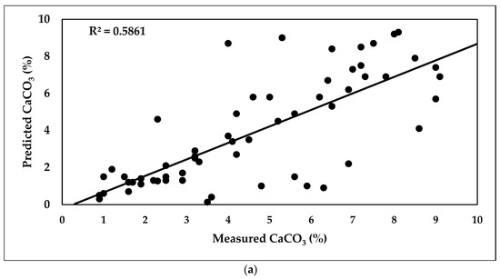
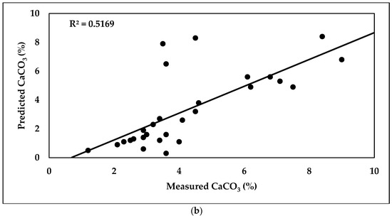
Figure 13.
Scatter plots of predicted (a) and measured (b) CaCO3 content using the PLSR model.
The CARS technique was applied to select the most correlated or effective bands as inputs to derive the PLSR model to determine various soil parameters, as presented in the next Equations (12) and (13).
Soil SOM parameter = 0.036 + 0.0631R496 − 0.0827R658 + 0.0372R779 + 0.0418R1089 − 0.0176R1417 − 0.0837R1871 + 0.0648R2423
CaCO3 parameter = 0.051 − 0.0298R470 − 0.0725R649 + 0.0427R802 + 0.0617R1161 − 0.08431R1421 − 0.0537R1854 + 0.07194R2362
3.6.2. Prediction of EF-Factor Using PLSR Model
The distribution of data points around the 1:1 line for both the calibration and validation data-sets indicates a good accuracy of the PLSR model in predicting the EF-Factor, with RMSE values of 0.0921 and 0.0836 Mg h MJ−1 mm−1 for the calibration and validation data-sets, respectively, as shown in Figure 14. Coefficient of determination (R2) values of 0.931 and 0.76 were found for the calibration and validation data-sets, respectively. The RPD values of 2.168 and 2.147 for the calibration and validation data-sets, respectively, provide information about the spread of the predicted EF-Factor values around the mean.
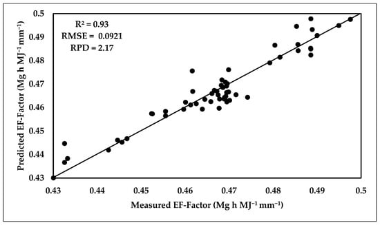
Figure 14.
Scatter plots of predicted versus referenced EF-Factor using the PLSR model for calibration data-set.
Equation (14) represents the PLSR model developed to determine the EF-Factor using selected spectral bands. The equation includes coefficients for each spectral band, denoted by R, and a constant term. The effective wavelengths selected for the PLSR model were determined based on the highest correlation with the EF-Factor, as measured by Pearson’s correlation coefficient (P-coefficient). The wavelengths reflected at 526, 688, 744, 1418, 1442, 2292, and 2374 nm were found to have the highest significant correlation with the EF-Factor, which are the selected bands for predicting the EF-Factor. In the equation, each spectral band is multiplied by its respective coefficient, which represents the strength and direction of the relationship between that band and the EF-Factor. The constant term (0.033) represents the intercept or baseline value. The coefficients for each band determine the weight or contribution of that band to the overall prediction.
where y is EF-Factor (soil erodibility) and R is spectral reflectance at band number/wavelength (nm).
y = 0.033 − 0.0261R526 + 0.0558R688 − 0.0333R744 − 0.0228R1418 + 0.0117R1442 − 0.01542R2292 + 0.0627R2374
3.6.3. Model Validation
The results presented in Figure 15 indicate that the PLSR model achieved an R2 value of 0.76, and a lower RMSE value of 0.0836 Mg h MJ−1 mm−1. These results suggest that combining the testing data with soil spectral information improves the accuracy of the EF-Factor prediction. The PLSR model, incorporating the selected spectral bands as inputs, provides a more precise estimation of the EF-Factor.
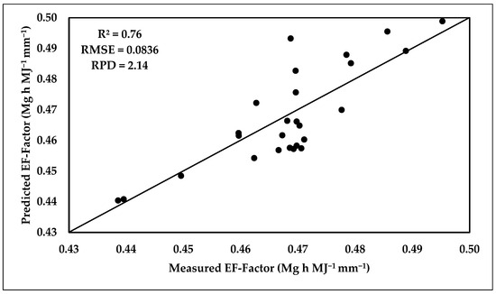
Figure 15.
Scatter plots of predicted versus referenced EF-Factor using the PLSR model for validation data-set.
3.6.4. Prediction of SOM, CaCO3, and EF-Factor Using the SVM Model
The obtained data of the SVM model for estimating SOM, CaCO3, and EF-Factor are shown in Table 5. Regarding the obtained results from the SVM model, the calibration dataset performed well in predicting SOM, with R2, RPD, and RMSE values of 0.63, 1.855, and 0.008%, respectively. In the validation stage, the SVM model had poor performance in estimating SOM, where the R2, RPD, and RMSE values were 0.35, 1.101, and 0.0827%, respectively.
The results of the SVM model in estimating the CaCO3 soil parameter reflected the reasonable accuracy of the calibration model (R2 = 0.51, RPD = 1.677, and RMSE = 0.175%). The validation model revealed that the low performance of SVR model improved in estimating the CaCO3 parameter, where the R2, RPD, and RMSE values were 0.29, 0.995, and 0.588%, respectively.
The performance of estimating the EF-Factor using the SVM model was poor in the calibration and validation datasets. The R2, RPD, and RMSE of the SVM calibration model were 0.52, 1.698, and 0.175, respectively, while in the validation model they were 0.12, 0.860, and 0.1903, respectively. The scatter plots of the predicted and measured soil parameters (SOM, CaCO3, and EF-Factor) are presented in Figure 16, Figure 17, Figure 18, Figure 19, Figure 20 and Figure 21.
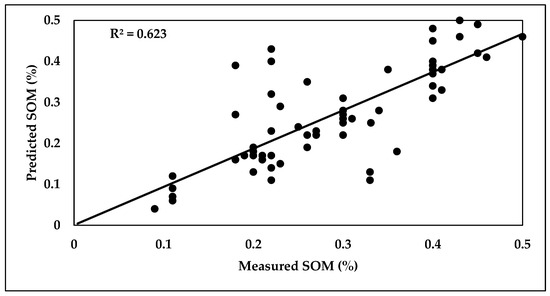
Figure 16.
Scatter plot between predicted and measured SOM of the SVM calibration model.
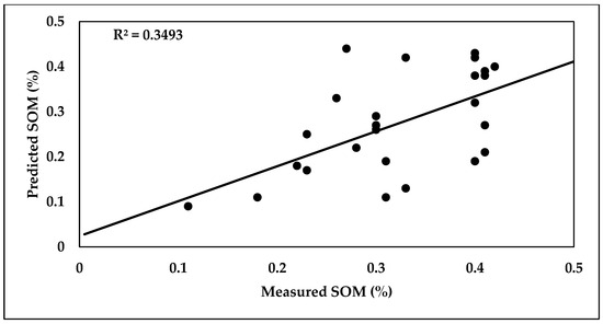
Figure 17.
Scatter plot between predicted and measured SOM of the SVM validation model.
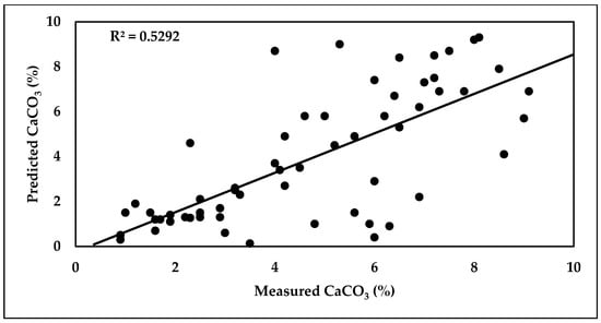
Figure 18.
Scatter plot between predicted and measured CaCO3 of the SVM Calibration model.
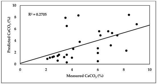
Figure 19.
Scatter plot between predicted and measured CaCO3 of the SVM validation model.
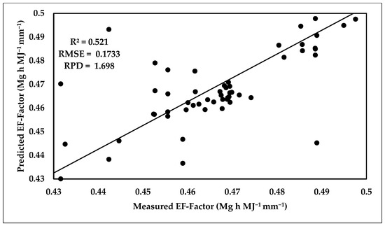
Figure 20.
Scatter plot between predicted and measured EF-Factor of the SVM calibration model.
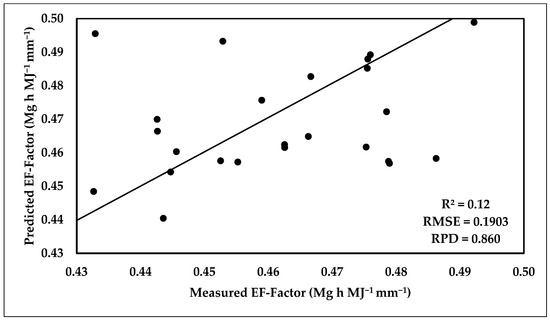
Figure 21.
Scatter plot between predicted and measured EF-Factor of the SVM validation model.
4. Discussion
In our study, the soil samples displayed a diverse range of measured properties including soil pH, CaCO3, EC, SOM, and soil particles (clay, sand, and silt contents). These findings reveal that the samples are slightly alkaline, potentially due to a limited presence of CaCO3, with a low to moderate level of dissolved salts or ions in the soil. Additionally, variations in SOM were observed among the soil samples. Regarding variability, CaCO3 exhibited the highest coefficient of variation (CV) value, signifying a significant variability in its content across the soil samples. Silt had the second highest CV value, while sand and pH had the lowest CV values, indicating less variability in their content among the soil samples; this finding is consistent with the result of El-Sayed et al. (2023) [56].
The lower value of EF-Factor, which represents the erosion factor, indicates that the soil is less susceptible to erosion, possibly due to factors such as high SOM content, good soil structure, and effective land management practices such as contouring or terracing. On the other hand, a higher EF-Factor value indicates a higher risk of soil erosion, which may be associated with factors such as poor soil structure, bare soil surfaces, or steep slopes. The mean EF-Factor in slope lands was significantly higher compared to other landforms which provide an overall representation of the erosion potential within the soil samples; however, it is important to consider other factors that can influence erosion, such as slope gradient, vegetation cover, and rainfall patterns. Additionally, the slope lands had the lowest amount of SOM, with a value of 0.01%. This indicates that the erosion factor was relatively consistent across the study area. However, the soils in slope lands, especially when plowed in the direction of the slopes, are indeed more susceptible to erosion due to their higher EF-Factor and lower SOM content, which is similar to the results found by Jiang et al. (2020) [33]. Soils with a high amount of OM, which are more sensitive to wind erosion, were found to have a positive correlation with the EF-Factor as well. This suggests that soils with a higher OM, which tend to have smaller and weaker aggregates, are more prone to erosion, leading to an increase in the EF-Factor [33]. A positive significant correlation was observed between the EF-Factor and CaCO3, which suggests that higher CaCO3 in the soil is associated with an increase in the EF-Factor [32], and a positive but weaker correlation was found between the EF-Factor and soil particles; these correlations indicate that soil particle composition, particularly the presence of organic matter (SOM), calcium carbonate (CaCO3), sand, and clay, can influence the EF-Factor and the susceptibility of soils to erosion [57]. As reported by Ostovari et al. (2018) [14], low correlation was observed between SOM and CaCO3 (r = 0.36). They mentioned that the high content of Ca2+ resulting from the CaCO3 is the main reason for the creation of large and stable aggregates which help in flocculating soil minerals. This process decreases the value of the EF-Factor.
According to the previous studies, soil texture, SOM, and CaCO3 are considered to be the most influential soil characteristics on spectral data [14,58].
The highest reflectance values were obtained from the less than 15% soil samples. This was because of high reflectance properties of the bright clay minerals (i.e., quartz and feldspar) [59]. Ostovari et al. (2018) [14] reported that sandy loam textured soils which contain bright minerals recorded higher reflectance values compared to other soils. On the other hands, high SOM content was found in the lowest slop areas compared to the topsoil. Moreover, the spectral reflectance is positively affected by the SOM content. Furthermore, the land use variability also affects SOM content. In lands with high slopes, high reflectance values are observed due to the erosion process which causes the transferring of fine soil fractions (clay, silt, and fine sand) [60].
At the spectral range between 700 and 2500 nm, CaCO3 can be distinguished, where strong diagnostic vibrational absorptions can be observed at 2300 –2350 nm. Other weaker bands occur near 2120–2160 nm, 1997–2000 nm, and 1850–1870 nm [61]. Multivariate calibrations must be applied for estimating soil parameters using the hyperspectral reflectance because of the complex absorption patterns caused by the large number of spectral bands [62]. Moreover, CaCO3 increases the brightness of the soil [63] and causes strong absorptions at 2300 to 2350 nm [64].
The results of this study agree with previous studies such as Lin et al. (2013) [20], which found that the wavelengths at 500, 700, 1220, 2200, and 2300 nm are sensitive to the SOM content of soil samples, while the wavelengths at 521, 951, 1417, 1937, and 2208 nm are related to soil erodibility.
The multivariate regression model (PLSR) was employed to predict soil parameters (SOM and CaCO3) using laboratory data and soil spectral data within the range of 350 to 2500 nm. Outliers were removed, and the datasets were validated before the modelling process. The data were divided into ten components in the internal PLSR process, with each component containing the same number of variables.
There are specific wavelengths or bands in the Vis-NIR spectrum which are significant for the assessment of some soil properties such as SOM and CaCO3 due to their ability to provide information about the molecular structure and composition of these soil properties. These bands are associated with the overtones and combinations of fundamental vibrations of chemical bonds such as N-H, C-H, and C-O. Generally, the specific bands that have been identified as significant for SOM estimation in the Vis-NIR region include 1650–1700 nm (methyl (–CH2) and methylene (=CH2) groups); 849, 917, 991, and 1007 nm (C-H stretching vibrations); 1681 and 2187 nm (overtones of O-H stretching vibrations); and 434, 2368, and 2490 nm (overtones of N-H stretching vibrations). These bands are associated with the overtones and combinations of fundamental vibrations of CaCO3 around 1300–1400 nm (overtone of the C-O stretching vibrations) and 2300–2500 nm (combination of C-O stretching and O-C-O bending vibrations). As the EF-Factor is in direct positive and linear relation with the SOM and CaCO3, it can be estimated using the vis-NIR spectral data.
The SOM laboratory data, as well as their corresponding reflectance, were used in developing the PLSR calibration model. The RMSE, RPD, and R2 of the PLSR calibration model were 0.0714%, 2.190, and 0.71, respectively. The RMSE, RPD, and R2 values of the PLSR validation model were 0.0683%, 2.137, and 0.58, respectively. These results reflect the ability of the PSR model and spectral data in estimating SOM with good accuracy [65,66,67]. Regarding the CaCO3, the R2, RPD, and RMSE values of the PLSR calibration model were 0.59, 2.562, and 0.0982%, respectively. The RMSE, RPD, and R2 values of the PLSR validation model were 0.4163%, 1.936, and 0.51, respectively. Our results are in the harmony with the findings of [68], who applied the PLSR to estimate CaCO3 based on the spectral data, where R2 and RMSE values were 0.518 and 3.39%, respectively. These values indicate the average deviation between the predicted and observed CaCO3 values in the validation dataset and suggest that the model has moderate to low predictive ability based on CaCO3.
The results demonstrate the accuracy and performance of PLSR model in estimating the EF-Factor using spectral reflectance data; the distribution of data points around the 1:1 line for both the calibration and validation datasets indicates a good accuracy of the PLSR model in predicting the EF-Factor, with RMSE values of 0.0921 and 0.0836 Mg h MJ−1 mm−1 for the calibration and validation datasets, respectively, which indicate the average deviation of the predicted EF-Factor values from the actual values. These low RMSE values suggest a high level of accuracy in the PLSR model’s predictions. The coefficient of determination (R2) values of 0.931 and 0.76 for the calibration and validation data-sets, respectively, indicate the proportion of the variance in the EF-Factor that can be explained by the PLSR model. The high R2 value for the calibration data-set suggests a very good performance of the model in predicting the EF-Factor, while the slightly lower R2 value for the validation data-set indicates a moderate performance. The RPD values of 0.0921 and 2.417 for the calibration and validation data-sets, respectively, provide information about the spread of the predicted EF-Factor values around the mean. These moderate RPD values suggest a relatively moderate variation in the predicted EF-Factor values, indicating a good precision of the PLSR model [14]. Most of the chosen wavelengths which were within spectra >540 nm were identified as the linked bands to the soil particles. Based on the information provided, it appears that the chosen wavelengths for predicting the EF-Factor using vis-NIR spectroscopy are mainly associated with soil particles rather than SOM and CaCO3 content. This suggests that the composition and distribution of soil particles, such as soil aggregates, clay, silt, and sand contents, have a more significant influence on of some soils characteristics prediction, and the rapid assessment of soil aggregate stability (AS) is crucial for enhancing our understanding of soil aggregate breakdown processes. This understanding is essential for effective soil erosion control planning [69].
The results indicate that the PLSR model achieved an R2 value of 0.76, indicating that it can explain 76% of the variance in predicting the EF-Factor. While this R2 value still considered a reasonably good performance in predicting the EF-Factor, the lower RMSE value of 0.0836 Mg h MJ−1 mm−1 for the PLSR model further supports its higher accuracy and indicates a smaller average deviation and higher precision of the model’s predictions.
Compared to the PLSR model, the SVM model’s performance was poor. There are some limitations in estimating SOM, CaCO3, and EF-Factor using the SVM model. The SVM model significantly relies on hyper parameters tuning of RBF, σ2, and other kernel parameters. In case of miss election of these parameters, low prediction accuracy is gained [70]. Due to the large number of the vis-NIR spectral variables, the SVM model cannot deal with this complexity in the datasets and is less efficient in prediction, especially when kernels’ nonlinear functions are used [71]. Compared to other regression models, the SVM model is hard to interpret, which has an effect on understanding the factors affecting the soil parameters such as SOM, CaCO3, and EF-Factor [72]. In case of nonlinear relationships between spectral variables and soil variables occur, the kernel function tuning can impact the SVM model’s performance [70]. Furthermore, the SVM model is sensitive to the data sets’ noises, which negatively affect the performance of the predictability, particularly when low signal-to-noise occurs [73].
These results suggest that combining the testing data with soil spectral information improves the accuracy of the EF-Factor prediction. The PLSR model, incorporating the selected spectral bands as inputs, provides a more precise estimation of the EF-Factor. The study by [33] supports the idea that combining vis-NIR spectroscopy with testing data can be meaningful in predicting the EF-Factor; this suggests that incorporating soil spectral information, along with field observations or measurements, can enhance the accuracy of EF-Factor predictions. Another study suggest that further efforts should be made to investigate other environmental variables that may influence the EF-Factor. These variables could include factors related to vegetation cover, as well as spatially related errors that may affect the accuracy of predictions [74].
The research work tried to estimate SOM, CaCO3, and EF-Factor using vis-NIR spectral data and (PLSR and SVM) prediction models. Regarding the current application of the vis-NIR integrated with PLSR for estimating EF-Factor, the achieved accuracy of the applied regression model is good.
Regarding the broader application, the generated regression equation of the developed PLSR model can be used for further estimation of soil erodibility in similar areas. Therefore, there is no need for analyzing soil parameters (clay, silt, sand, SOM, and CaCO3) again using the traditional methods of analysis. Only vis-NIR data are required to be calculated through the developed PL-regression equations to estimate the EF-Factor of unknown soil samples.
On the other hand, the developed model may not be suitable for all areas because of heterogeneity of the soil data as well as different environmental factors. As this research work is empirical and the datasets size is low, more studies must be carried out using the same technology with an aim to get more data sets and run more various models for enhancing the accuracy of predicting EF-Factor in different study sites. It should be mentioned that these techniques are still empirical, and more effort and research studies are required for increasing the accuracy of the used models and datasets [75].
Land management and erosion control strategies in arid lands have significant practical implications for the sustainability of these ecosystems and the communities that depend on them. In arid regions, depletion of soil organic matter leads to a decrease in soil moisture-holding capacity, a reduction in crops, and an increase in soil erosion, which can exacerbate desertification and land degradation. Effective land management strategies in arid lands include sustainable land management practices, such as the use of fodder crops to protect the soil from wind and water erosion, enhance soil fertility, improve plant and habitat diversity, and reduce soil and water losses. These sustainable land management practices can also help to mitigate the impacts of climate change in arid lands by increasing the resilience of ecosystems and communities to extreme weather events and other climate-related stressors. For example, these practices can help to reduce soil erosion and improve soil health, which can enhance the capacity of soils to sequester carbon and regulate water cycles. These practices can also help to maintain or enhance the productivity of agricultural lands, which can contribute to food security and livelihoods in arid regions [21].
Erosion control strategies in arid lands can include the use of physical barriers, such as terraces, check dams, and vegetation strips, to reduce the velocity of water flow and promote infiltration and sediment deposition [61]. These strategies can also involve the use of agronomic practices, such as conservation tillage, crop rotation, and cover cropping, to reduce soil erosion and enhance soil health. The selection and implementation of erosion control strategies should be based on site-specific conditions, such as topography, soil type, climate, and land use. Effective land management and erosion control strategies in arid lands require the integration of scientific knowledge, traditional practices, and local knowledge, as well as the participation of stakeholders, including farmers, pastoralists, and policymakers. These strategies should also consider the social, economic, and cultural contexts of arid lands and aim to balance the needs and interests of different stakeholders while promoting sustainable development and poverty reduction.
The use of Vis-NIR spectroscopy for estimating EF-Factor in soil is a significant tool for land management and erosion control strategies in arid lands. By providing rapid and accurate estimates of EF-Factor and other soil properties, Vis-NIR spectroscopy can help land managers make more informed decisions about soil conservation and erosion control strategies [75].
5. Conclusions
The current study aimed to predict the wind-erodible fraction (EF-Factor) using vis-NIR spectroscopy, soil texture, and chemical properties, employing PLSR and SVM models. The results indicated that sloped lands with a SOM content of 0.01% had the highest EF-Factor values. The Pearson’s correlation coefficient (r) between the EF-Factor and spectral data was examined among the soil properties, and SOM showed the highest positive correlation with the EF-Factor, with a correlation coefficient of 0.814 (p < 0.01). The results showed that the spectral responses of soil calcium carbonate were observed in separate places in the wavelength, namely 570, 649, 802, 1161, 1421, 1854, and 2362 nm, respectively; the wavelengths with the SOM parameter were 496, 658, 779, 1089, 1417, 1871, and 2423 nm, respectively, and the EF-factor showed the highest significant correlation with spectral reflectance values at 526, 688, 744, 1418, 1442, 2292, and 2374 nm, respectively. The accuracy and performance of the PLSR model in estimating the EF-Factor using spectral reflectance data and the distribution of data points for both the calibration and validation datasets indicates a good accuracy of the PLSR model, with RMSE values of 0.0921 and 0.0836 Mg h MJ−1 mm−1, respectively, and the coefficient of determination (R2) values, which were 0.931 and 0.76, indicate the proportion of the variance in the EF-Factor that can be explained by the PLSR model; the RPD values were 0.0921 and 2.417 for the calibration and validation data-sets, respectively. The effective wavelengths selected for the PLSR model were determined based on the highest correlation with the EF-Factor, found at 526, 688, 744, 1418, 1442, 2292, and 2374 nm, respectively. The chosen wavelengths for predicting the EF-Factor using vis-NIR spectroscopy are mainly associated with soil particles rather than SOM and CaCO3 content.
The SVM model performance was poor in estimating SOM, CaCO3, and EF-Factor. The validation R2 of these three soil parameters were 0.35, 0.29, and 0.12, respectively. Compared to the PLSR model, the SVM model was not able to estimate the soil parameters properly.
Overall, the study highlights the potential of vis-NIR spectroscopy combined with soil sample data for predicting the EF-Factor and other soil properties. It also emphasizes the importance of considering additional variables and employing advanced modelling techniques to improve prediction accuracy and enhance the understanding of soil erosion processes in specific ecosystems. In summary, the study underscores the significance of advanced technologies such as vis-NIR spectroscopy in soil prediction models and suggests avenues for further research and improvement in predicting soil erosion factors.
Author Contributions
Conceptualization, A.H.A.-E., M.A.E.-S., M.E.F., M.Z., S.A.H.S., M.D., A.S. and A.R.A.M.; methodology, A.H.A.-E., M.A.E.-S., M.E.F., M.D., A.S. and A.R.A.M.; software, A.H.A.-E., M.A.E.-S., M.E.F., M.Z., S.A.H.S., M.D., A.S. and A.R.A.M.; validation, A.H.A.-E., M.A.E.-S., M.E.F., M.Z., S.A.H.S., M.D., A.S. and A.R.A.M.; formal analysis, A.H.A.-E., M.A.E.-S., M.E.F., M.Z., S.A.H.S., M.D., A.S. and A.R.A.M.; investigation, A.H.A.-E.; resources, A.H.A.-E., M.A.E.-S., M.E.F., M.Z., S.A.H.S., M.D., A.S. and A.R.A.M.; data curation, A.H.A.-E., M.A.E.-S., M.E.F., M.Z., S.A.H.S., M.D., A.S. and A.R.A.M.; writing․original draft preparation, A.H.A.-E., M.A.E.-S., M.E.F., M.Z., S.A.H.S., M.D., A.S. and A.R.A.M.; writing․review and editing, A.H.A.-E., M.A.E.-S., M.E.F., M.Z., S.A.H.S., M.D., A.S. and A.R.A.M.; visualization, A.H.A.-E., M.A.E.-S., M.E.F., M.Z., S.A.H.S., M.D., A.S. and A.R.A.M.; supervision, M.E.F., A.S. and A.R.A.M.; project administration, M.E.F., A.R.A.M. and A.S.; funding acquisition, A.H.A.-E., M.A.E.-S., M.E.F., M.Z., S.A.H.S., M.D., A.S. and A.R.A.M. All authors have read and agreed to the published version of the manuscript.
Funding
This research received no external funding.
Institutional Review Board Statement
Not applicable.
Informed Consent Statement
Not applicable.
Data Availability Statement
Data are contained within the article.
Acknowledgments
The manuscript presented a scientific collaboration between scientific institutions in three countries (Egypt, Algeria and Italy). The authors would like to thank the Aswan, Sohag, Al Azhar, Assiut Universities, National Higher Agronomic School, SAFE-Università degli Studi della Basilicata and National Authority for Remote Sensing and Space Science (NARSS) for funding the satellite data and the field survey.
Conflicts of Interest
The authors declare no conflicts of interest.
References
- Riedel, F.; Denk, M.; Müller, I.; Barth, N.; Gläßer, C. Prediction of soil parameters using the spectral range between 350 and 15,000 nm: A case study based on the Permanent Soil Monitoring Program in Saxony, Germany. Geoderma 2018, 315, 188–198. [Google Scholar] [CrossRef]
- Rossel, R.V.; McGlynn, R.; McBratney, A. Determining the composition of mineral-organic mixes using UV–vis–NIR diffuse reflectance spectroscopy. Geoderma 2006, 137, 70–82. [Google Scholar] [CrossRef]
- Renard, K.G. Predicting Soil Erosion by Water: A Guide to Conservation Planning with the Revised Universal Soil Loss Equation (RUSLE); US Department of Agriculture, Agricultural Research Service: Beltsville, MD, USA, 1997.
- Millward, A.A.; Mersey, J.E. Adapting the RUSLE to model soil erosion potential in a mountainous tropical watershed. Catena 1999, 38, 109–129. [Google Scholar] [CrossRef]
- Selmy, S.A.; Abd Al-Aziz, S.H.; Jiménez-Ballesta, R.; García-Navarro, F.J.; Fadl, M.E. Soil quality assessment using multivariate approaches: A case study of the dakhla oasis arid lands. Land 2021, 10, 1074. [Google Scholar] [CrossRef]
- Wischmeier, W.H.; Smith, D.D. Predicting Rainfall Erosion Losses: A Guide to Conservation Planning; Department of Agriculture, Science and Education Administration: Washington, DC, USA, 1978.
- Nikseresht, F.; Honarbakhsh, A.; Ostovari, Y.; Afzali, S.F. Model development to predict CEC using the intelligence data mining approaches. Commun. Soil Sci. Plant Anal. 2019, 50, 2178–2189. [Google Scholar] [CrossRef]
- Mirzaee, S.; Ghorbani-Dashtaki, S.; Kerry, R. Comparison of a spatial, spatial and hybrid methods for predicting inter-rill and rill soil sensitivity to erosion at the field scale. Catena 2020, 188, 104439. [Google Scholar] [CrossRef]
- Wang, G.; Fang, Q.; Teng, Y.; Yu, J. Determination of the factors governing soil erodibility using hyperspectral visible and near-infrared reflectance spectroscopy. Int. J. Appl. Earth Obs. Geoinf. 2016, 53, 48–63. [Google Scholar] [CrossRef]
- Afriyie, E.; Verdoodt, A.; Mouazen, A.M. Potential of visible-near infrared spectroscopy for the determination of three soil aggregate stability indices. Soil Tillage Res. 2022, 215, 105218. [Google Scholar] [CrossRef]
- de Santana, F.B.; de Souza, A.M.; Poppi, R.J. Visible and near infrared spectroscopy coupled to random forest to quantify some soil quality parameters. Spectrochim. Acta Part A Mol. Biomol. Spectrosc. 2018, 191, 454–462. [Google Scholar] [CrossRef] [PubMed]
- Kim, I.; Pullanagari, R.; Deurer, M.; Singh, R.; Huh, K.; Clothier, B. The use of visible and near-infrared spectroscopy for the analysis of soil water repellency. Eur. J. Soil Sci. 2014, 65, 360–368. [Google Scholar] [CrossRef]
- Afriyie, E.; Verdoodt, A.; Mouazen, A.M. Data fusion of visible near-infrared and mid-infrared spectroscopy for rapid estimation of soil aggregate stability indices. Comput. Electron. Agric. 2021, 187, 106229. [Google Scholar] [CrossRef]
- Ostovari, Y.; Ghorbani-Dashtaki, S.; Bahrami, H.-A.; Abbasi, M.; Dematte, J.A.M.; Arthur, E.; Panagos, P. Towards prediction of soil erodibility, SOM and CaCO3 using laboratory Vis-NIR spectra: A case study in a semi-arid region of Iran. Geoderma 2018, 314, 102–112. [Google Scholar] [CrossRef]
- Khayamim, F.; Khademi, H.; Stenberg, B.; Wetterlind, J. Capability of vis-NIR spectroscopy to predict selected chemical soil properties in Isfahan Province. JWSS-Isfahan Univ. Technol. 2015, 19, 81–92. [Google Scholar] [CrossRef]
- Bellon-Maurel, V.; McBratney, A. Near-infrared (NIR) and mid-infrared (MIR) spectroscopic techniques for assessing the amount of carbon stock in soils–Critical review and research perspectives. Soil Biol. Biochem. 2011, 43, 1398–1410. [Google Scholar] [CrossRef]
- Dufréchou, G.; Grandjean, G.; Bourguignon, A. Geometrical analysis of laboratory soil spectra in the short-wave infrared domain: Clay composition and estimation of the swelling potential. Geoderma 2015, 243, 92–107. [Google Scholar] [CrossRef]
- Gomez, C.; Lagacherie, P.; Coulouma, G. Continuum removal versus PLSR method for clay and calcium carbonate content estimation from laboratory and airborne hyperspectral measurements. Geoderma 2008, 148, 141–148. [Google Scholar] [CrossRef]
- Chabrillat, S.; Goetz, A.F.; Krosley, L.; Olsen, H.W. Use of hyperspectral images in the identification and mapping of expansive clay soils and the role of spatial resolution. Remote Sens. Environ. 2002, 82, 431–445. [Google Scholar] [CrossRef]
- Lin, C.; Zhou, S.-L.; Wu, S.-H. Using hyperspectral reflectance to detect different soil erosion status in the Subtropical Hilly Region of Southern China: A case study of Changting, Fujian Province. Environ. Earth Sci. 2013, 70, 1661–1670. [Google Scholar] [CrossRef]
- Sayed, Y.A.; Fadl, M.E. Agricultural sustainability evaluation of the new reclaimed soils at Dairut Area, Assiut, Egypt using GIS modeling. Egypt. J. Remote Sens. Space Sci. 2021, 24, 707–719. [Google Scholar] [CrossRef]
- Natural Resources Conservation Service; Agriculture Department (Eds.) Keys to Soil Taxonomy; Government Printing Office: Washington, DC, USA, 2010. [Google Scholar]
- Embabi, N.S. The karstified carbonate platforms in the Western Desert. In Landscapes and Landforms of Egypt: Landforms and Evolution; Springer: Cham, Switzerland, 2018; pp. 85–104. [Google Scholar] [CrossRef]
- Jahn, R.; Blume, H.; Asio, V.; Spaargaren, O.; Schad, P. Guidelines for Soil Description, 4th ed.; FAO: Rome, Italy, 2006; p. 109. [Google Scholar]
- Staff, S.S. Keys to Soil Taxonomy; United States Department of Agriculture: Washington, DC, USA, 2014.
- Gee, G.W.; Or, D. 2.4 Particle-size analysis. Methods Soil Anal. Part 4 Phys. Methods 2002, 5, 255–293. [Google Scholar]
- Walkley, A.; Black, I.A. An examination of the Degtjareff method for determining soil organic matter, and a proposed modification of the chromic acid titration method. Soil Sci. 1934, 37, 29–38. [Google Scholar] [CrossRef]
- Wischmeier, W.H. A rainfall erosion index for a universal soil-loss equation. Soil Sci. Soc. Am. J. 1959, 23, 246–249. [Google Scholar] [CrossRef]
- Fryrear, D.; Krammes, C.; Williamson, D.; Zobeck, T. Computing the wind erodible fraction of soils. J. Soil Water Conserv. 1994, 49, 183–188. [Google Scholar]
- Weidong, L.; Baret, F.; Xingfa, G.; Qingxi, T.; Lanfen, Z.; Bing, Z. Relating soil surface moisture to reflectance. Remote Sens. Environ. 2002, 81, 238–246. [Google Scholar] [CrossRef]
- Rossel, R.V.; Behrens, T. Using data mining to model and interpret soil diffuse reflectance spectra. Geoderma 2010, 158, 46–54. [Google Scholar] [CrossRef]
- Ben-Dor, E.; Banin, A. Near-infrared analysis as a rapid method to simultaneously evaluate several soil properties. Soil Sci. Soc. Am. J. 1995, 59, 364–372. [Google Scholar] [CrossRef]
- Jiang, Q.; Chen, Y.; Hu, J.; Liu, F. Use of visible and near-infrared reflectance spectroscopy models to determine soil erodibility factor (K) in an ecologically restored watershed. Remote Sens. 2020, 12, 3103. [Google Scholar] [CrossRef]
- Wold, S.; Sjöström, M.; Eriksson, L. PLS-regression: A basic tool of chemometrics. Chemom. Intell. Lab. Syst. 2001, 58, 109–130. [Google Scholar] [CrossRef]
- Rouse, J.W.; Haas, R.H.; Schell, J.A.; Deering, D.W. Monitoring vegetation systems in the Great Plains with ERTS. NASA Spec. Publ. 1974, 351, 309. [Google Scholar]
- Geladi, P.; Kowalski, B.R. Partial least-squares regression: A tutorial. Anal. Chim. Acta 1986, 185, 1–17. [Google Scholar] [CrossRef]
- Montgomery, D.C.; Peck, E.A.; Vining, G.G. Introduction to Linear Regression Analysis; John Wiley & Sons: Oak Brook, IL, USA, 2021; p. 704. [Google Scholar]
- Martens, H.; Naes, T. Multivariate Calibration; John Wiley and Sons: Chichester, UK, 1992. [Google Scholar]
- Malone, B.P.; Minasny, B.; Odgers, N.P.; McBratney, A.B. Using model averaging to combine soil property rasters from legacy soil maps and from point data. Geoderma 2014, 232, 34–44. [Google Scholar] [CrossRef]
- Diks, C.G.; Vrugt, J.A. Comparison of point forecast accuracy of model averaging methods in hydrologic applications. Stoch. Environ. Res. Risk Assess. 2010, 24, 809–820. [Google Scholar] [CrossRef]
- Dondeyne, S.; Vanierschot, L.; Langohr, R.; Van Ranst, E.; Deckers, S. The Soil Map of the Flemish Region Converted to the 3rd Edition of the World Reference Base for Soil Resources. 2014. Available online: https://scholar.google.com/citations?view_op=view_citation&hl=en&user=Aeo6mzgAAAAJ&citation_for_view=Aeo6mzgAAAAJ:NhqRSupF_l8C (accessed on 25 March 2024).
- Granger, C.W.; Ramanathan, R. Improved methods of combining forecasts. J. Forecast. 1984, 3, 197–204. [Google Scholar] [CrossRef]
- Bates, J.M.; Granger, C.W. The combination of forecasts. J. Oper. Res. Soc. 1969, 20, 451–468. [Google Scholar] [CrossRef]
- Hoeting, J.A.; Madigan, D.; Raftery, A.E.; Volinsky, C.T. Bayesian model averaging: A tutorial (with comments by M. Clyde, David Draper and EI George, and a rejoinder by the authors. Stat. Sci. 1999, 14, 382–417. [Google Scholar] [CrossRef]
- Bellon-Maurel, V.; Fernandez-Ahumada, E.; Palagos, B.; Roger, J.M.; McBratney, A. Critical review of chemometric indicators commonly used for assessing the quality of the prediction of soil attributes by NIR spectroscopy. TrAC Trends Anal. Chem. 2010, 29, 1073–1081. [Google Scholar] [CrossRef]
- Rossel, R.V.; Walvoort, D.J.J.; McBratney, A.B.; Janik, L.J.; Skjemstad, J.O. Visible, near infrared, mid infrared or combined diffuse reflectance spectroscopy for simultaneous assessment of various soil properties. Geoderma 2006, 131, 59–75. [Google Scholar] [CrossRef]
- Box, G.E.; Cox, D.R. An analysis of transformations. J. R. Stat. Soc. Ser. B Stat. Methodol. 1964, 26, 211–243. [Google Scholar] [CrossRef]
- Enders, A.; North, N.; Clark, J.; Allen, H. Saccharide concentration prediction from proxy-sea surface microlayer samples analyzed via ATR-ATR-FTIR spectroscopy and quantitative machine learning. Anal. Chem. 2023, preprint. [Google Scholar] [CrossRef]
- Stenberg, B. Effects of soil sample pretreatments and standardized rewetting as interacted with sand classes on Vis-NIR predictions of clay and soil organic carbon. Geoderma 2010, 158, 15–22. [Google Scholar] [CrossRef]
- Vapnik, V. The Nature of Statistical Learning Theory; Springer: New York, NY, USA, 2000; p. 314. [Google Scholar] [CrossRef]
- De Brabanter, K.; De Brabanter, J.; Gijbels, I.; De Moor, B. Derivative estimation with local polynomial fitting. J. Mach. Learn. Res. 2013, 14, 281–301. [Google Scholar]
- Stone, M. Cross-validation and multinomial prediction. Biometrika 1974, 61, 509–515. [Google Scholar] [CrossRef]
- Suykens, J.A.; De Brabanter, J.; Lukas, L.; Vandewalle, J. Weighted least squares support vector machines: Robustness and sparse approximation. Neurocomputing 2002, 48, 85–105. [Google Scholar] [CrossRef]
- Mouazen, A.M.; Kuang, B.; De Baerdemaeker, J.; Ramon, H. Comparison among principal component, partial least squares and back propagation neural network analyses for accuracy of measurement of selected soil properties with visible and near infrared spectroscopy. Geoderma 2010, 158, 23–31. [Google Scholar] [CrossRef]
- Jobson, J.D. Applied Multivariate Data Analysis: Regression and Experimental Design; Springer Science & Business Media: Berlin/Heidelberg, Germany, 2012. [Google Scholar]
- Li, S.; Ji, W.; Chen, S.; Peng, J.; Zhou, Y.; Shi, Z. Potential of VIS-NIR-SWIR spectroscopy from the Chinese Soil Spectral Library for assessment of nitrogen fertilization rates in the paddy-rice region, China. Remote Sens. 2015, 7, 7029–7043. [Google Scholar] [CrossRef]
- El-Sayed, M.A.; Abd-Elazem, A.H.; Moursy, A.R.; Mohamed, E.S.; Kucher, D.E.; Fadl, M.E. Integration Vis-NIR Spectroscopy and Artificial Intelligence to Predict Some Soil Parameters in Arid Region: A Case Study of Wadi Elkobaneyya, South Egypt. Agronomy 2023, 13, 935. [Google Scholar] [CrossRef]
- Bonilla, C.A.; Johnson, O.I. Soil erodibility mapping and its correlation with soil properties in Central Chile. Geoderma 2012, 189, 116–123. [Google Scholar] [CrossRef]
- Rossel, R.V. Robust modelling of soil diffuse reflectance spectra by “bagging-partial least squares regression”. J. Near Infrared Spectrosc. 2007, 15, 39–47. [Google Scholar] [CrossRef]
- Bowers, S.A. Reflection of Radiant Energy from Soils; Kansas State University: Manhattan, AR, USA, 1971. [Google Scholar]
- Selmy, S.A.; Abd Al-Aziz, S.H.; Jiménez-Ballesta, R.; García-Navarro, F.J.; Fadl, M.E. Modeling and assessing potential soil erosion hazards using USLE and wind erosion models in integration with gis techniques: Dakhla oasis, Egypt. Agriculture 2021, 11, 1124. [Google Scholar] [CrossRef]
- Clark, R.N.; Rencz, A.N. Spectroscopy of rocks and minerals, and principles of spectroscopy. Man. Remote Sens. 1999, 3, 3–58. [Google Scholar]
- He, G.; Zhang, Z.; Wu, X.; Cui, M.; Zhang, J.; Huang, X. Adsorption of heavy metals on soil collected from Lixisol of typical karst areas in the presence of CaCO3 and soil clay and their competition behavior. Sustainability 2020, 12, 7315. [Google Scholar] [CrossRef]
- Girard, M.; Girard, C. Télédétection Appliquée: Zones Tempérées et Intertropicales; Elsevier Mason SAS: Amsterdam, The Netherlands, 1989. [Google Scholar]
- Hunt, G.R. Visible and near-infrared spectra of minerals and rocks: III. Oxides and hydro-oxides. Mod. Geol. 1971, 2, 195–205. [Google Scholar]
- Yang, M.; Xu, D.; Chen, S.; Li, H.; Shi, Z. Evaluation of machine learning approaches to predict soil organic matter and pH using Vis-NIR spectra. Sensors 2019, 19, 263. [Google Scholar] [CrossRef] [PubMed]
- Mohamed, E.S.; Baroudy, A.A.E.; El-beshbeshy, T.; Emam, M.; Belal, A.; Elfadaly, A.; Aldosari, A.A.; Ali, A.M.; Lasaponara, R. Vis-nir spectroscopy and satellite landsat-8 oli data to map soil nutrients in arid conditions: A case study of the northwest coast of egypt. Remote Sens. 2020, 12, 3716. [Google Scholar] [CrossRef]
- Zhang, X.; Xue, J.; Xiao, Y.; Shi, Z.; Chen, S. Towards Optimal Variable Selection Methods for Soil Property Prediction Using a Regional Soil Vis-NIR Spectral Library. Remote Sens. 2023, 15, 465. [Google Scholar] [CrossRef]
- Alomar, S.; Mireei, S.A.; Hemmat, A.; Masoumi, A.A.; Khademi, H. Prediction and variability mapping of some physicochemical characteristics of calcareous topsoil in an arid region using Vis–SWNIR and NIR spectroscopy. Sci. Rep. 2022, 12, 1–17. [Google Scholar] [CrossRef] [PubMed]
- Saha, P.; Debnath, P.; Thomas, P. Prediction of fresh and hardened properties of self-compacting concrete using support vector regression approach. Neural Comput. Appl. 2020, 32, 7995–8010. [Google Scholar] [CrossRef]
- Wu, J.; Wang, Y.G.; Tian, Y.C.; Burrage, K.; Cao, T. Support vector regression with asymmetric loss for optimal electric load forecasting. Energy 2021, 223, 119969. [Google Scholar] [CrossRef]
- Chaibi, M.; Benghoulam, E.M.; Tarik, L.; Berrada, M.; Hmaidi, A.E. An interpretable machine learning model for daily global solar radiation prediction. Energies 2021, 14, 7367. [Google Scholar] [CrossRef]
- Sabzekar, M.; Hasheminejad, S.M.H. Robust regression using support vector regressions. Chaos Solitons Fractals 2021, 144, 110738. [Google Scholar] [CrossRef]
- Afriyie, E.; Verdoodt, A.; Mouazen, A.M. Estimation of aggregate stability of some soils in the loam belt of Belgium using mid-infrared spectroscopy. Sci. Total Environ. 2020, 744, 140727. [Google Scholar] [CrossRef]
- Bishop, C.M. Pattern Recognition and Machine Learning; Springer: Berlin/Heidelberg, Germany, 2006. [Google Scholar]
Disclaimer/Publisher’s Note: The statements, opinions and data contained in all publications are solely those of the individual author(s) and contributor(s) and not of MDPI and/or the editor(s). MDPI and/or the editor(s) disclaim responsibility for any injury to people or property resulting from any ideas, methods, instructions or products referred to in the content. |
© 2024 by the authors. Licensee MDPI, Basel, Switzerland. This article is an open access article distributed under the terms and conditions of the Creative Commons Attribution (CC BY) license (https://creativecommons.org/licenses/by/4.0/).