
Identification of Soil Arsenic Contamination in Rice Paddy Field Based on Hyperspectral Reflectance Approach


Abstract
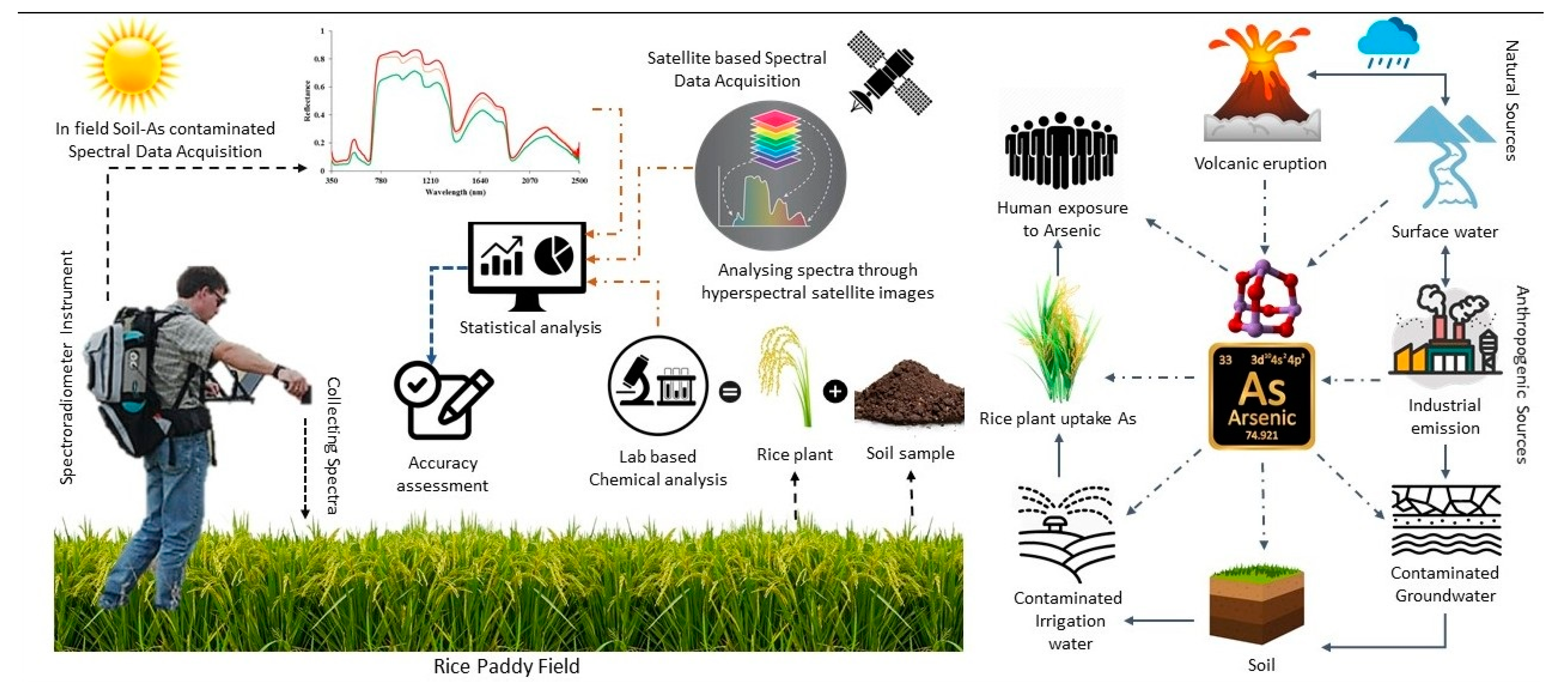
:1. Introduction of Arsenic Contaminations
2. Arsenic Concentration in Rice Plants
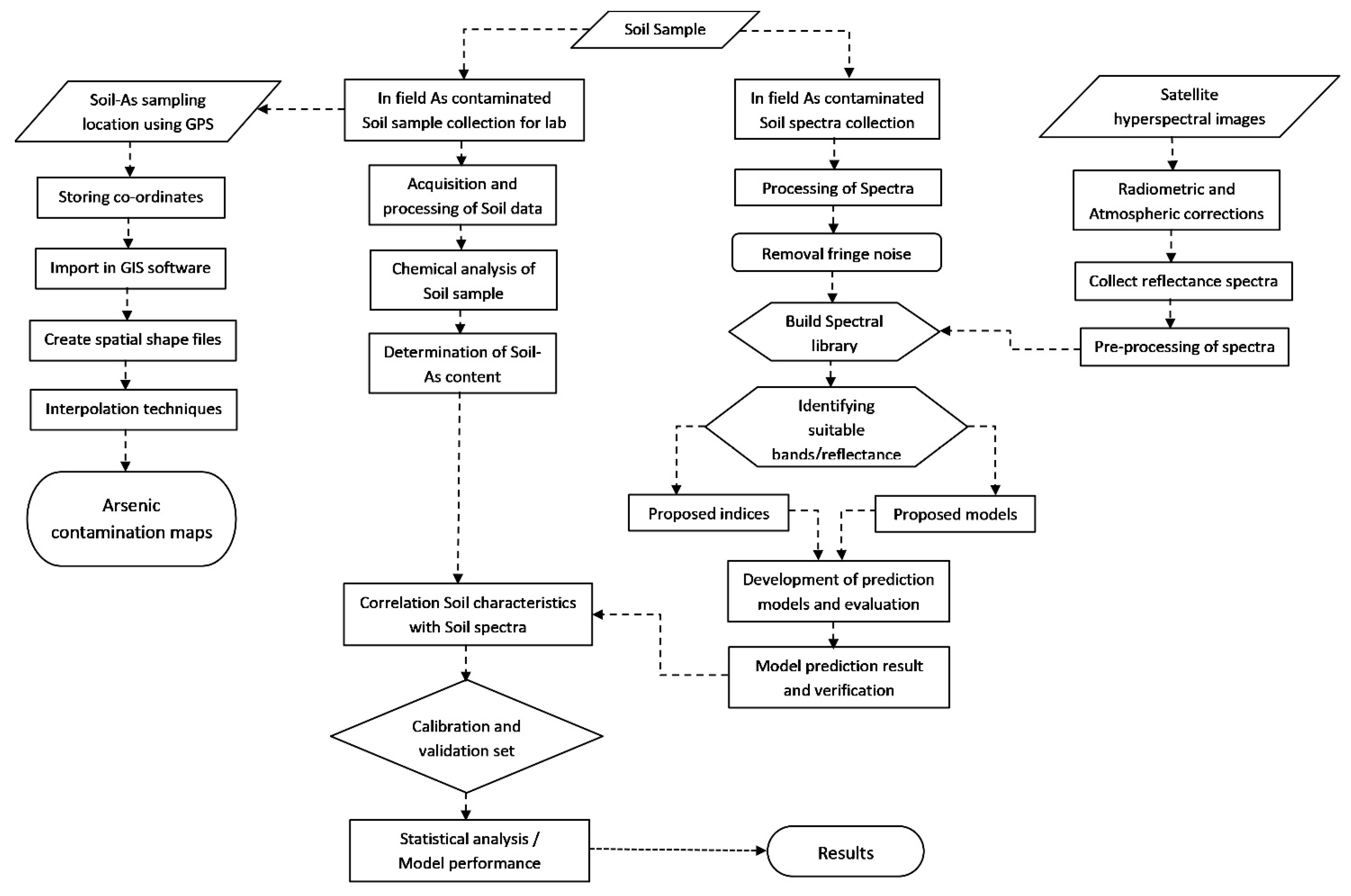
3. Use of Remote Sensing
3.1. Hyperspectral Reflectance Measurement
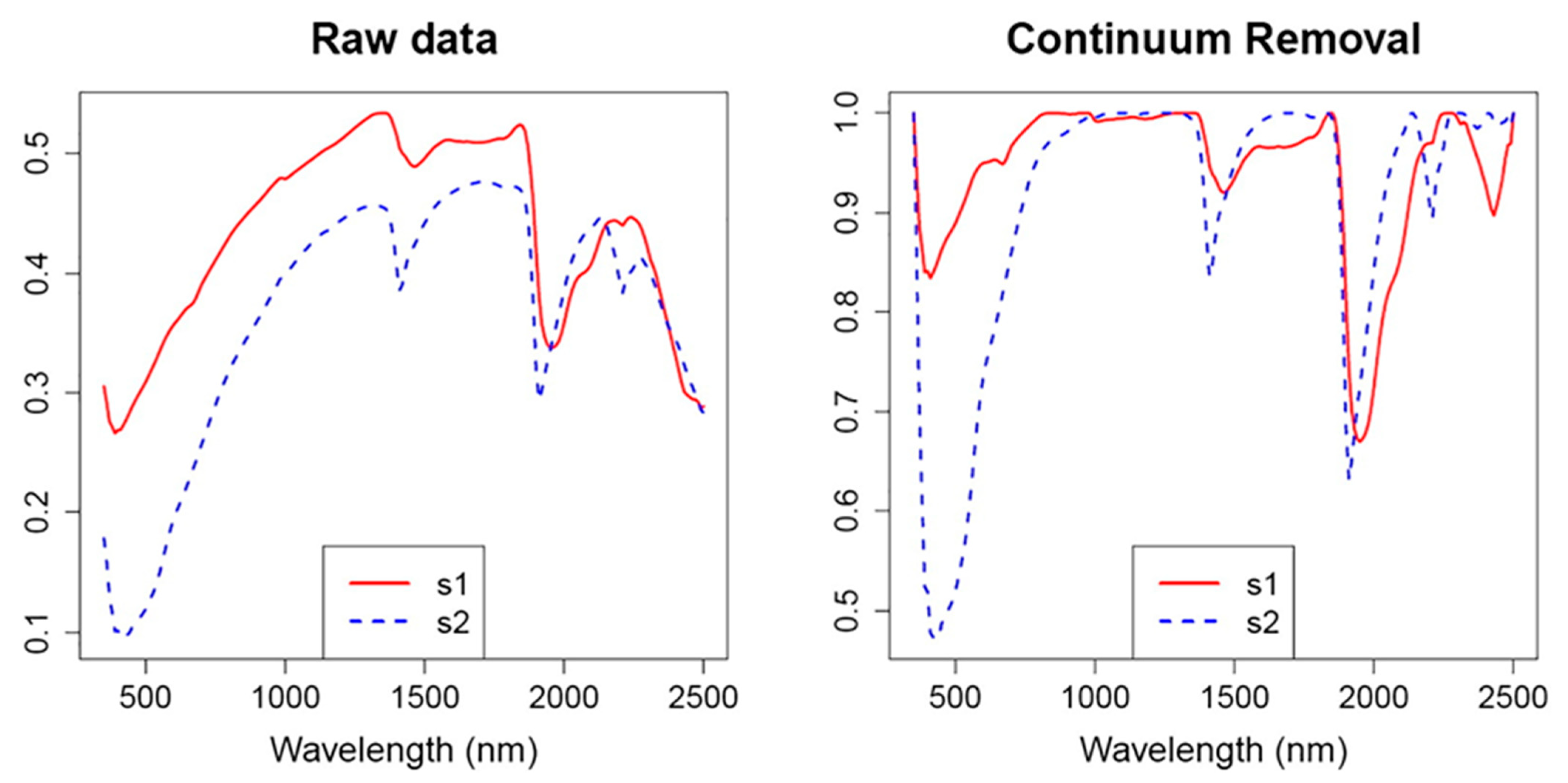
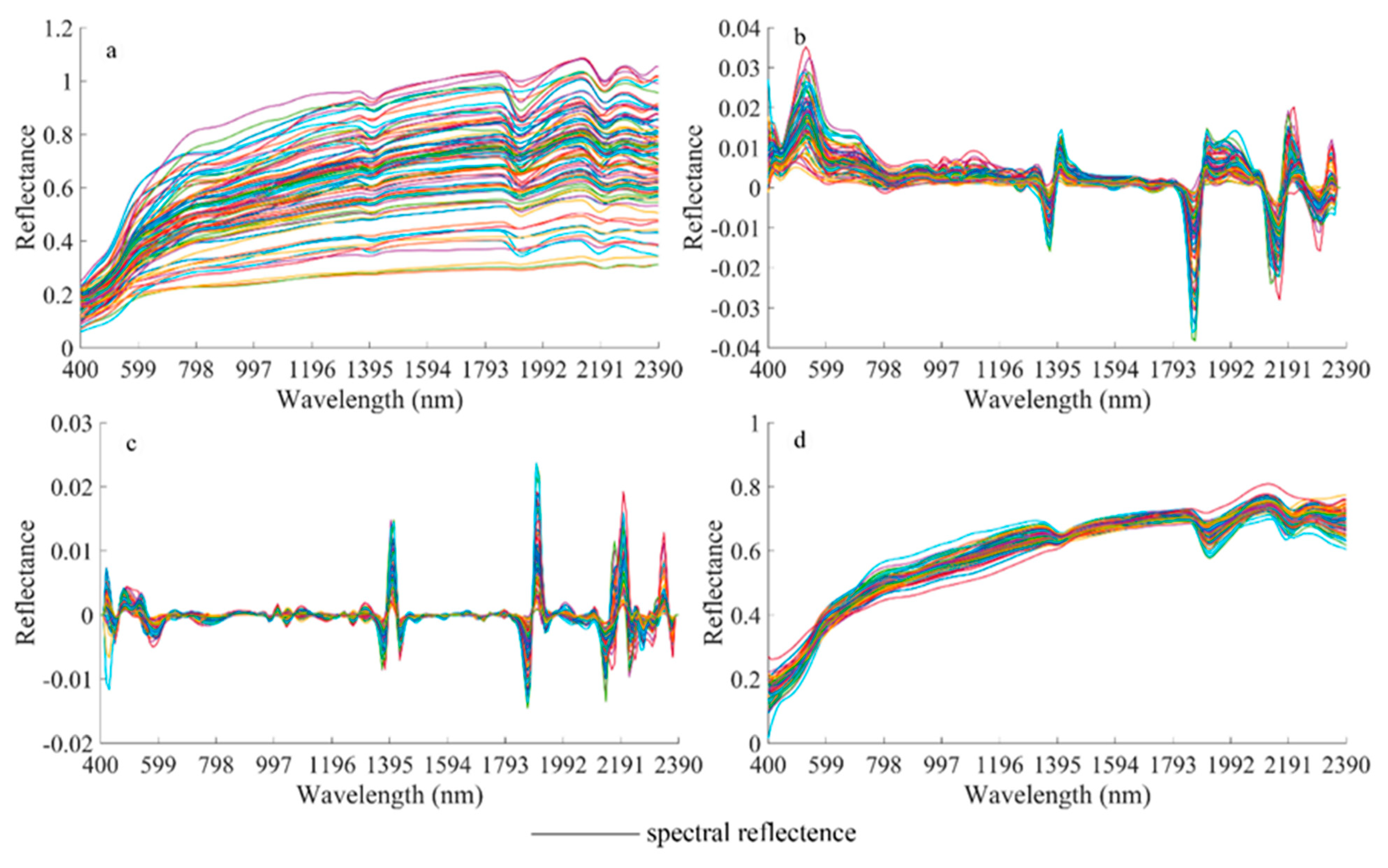
Spectral Data Pretreatments
- Scr = Continuum-removed spectra
- S = Original spectrum
- C = Continuum curve

3.2. Spectra Collection
4. Methods for Arsenic Measurement
4.1. Hydroponic Method for Evaluating Leaf and Canopy Reflectance of Stressed Rice Plants for As Contaminants
4.2. Estimation of Soil As Using Generated Model and Hyperspectral Remote Sensing
4.3. Visible Near-Infrared Diffuse Reflectance Spectroscopy (VisNIR-DRS) Approach
4.4. Fuzzy Overlay and Spatial Anisotropy Approach
4.5. Multivariate Hyperspectral Vegetation Indices
5. Limitations of Hyperspectral Remote Sensing Data
6. Conclusions
Author Contributions
Funding
Institutional Review Board Statement
Informed Consent Statement
Data Availability Statement
Acknowledgments
Conflicts of Interest
References
- Woolson, E.A. Arsenical pesticides. In Proceedings of the 168th Meeting of the American Chemical Society, Atlantic City, NJ, USA, 9 September 1974. [Google Scholar]
- Mandal, B.K.; Suzuki, K.T. Arsenic round the world: A review. Talanta 2002, 58, 201–235. [Google Scholar] [CrossRef]
- Gulledge, J.H.; O’Connor, J.T. Removal of Arsenic (V) From Water by Adsorption on Aluminum and Ferric Hydroxides. J.-Am. Water Work. Assoc. 1973, 65, 548–552. [Google Scholar] [CrossRef]
- Kabata-Pendias, A.; Pendias, H. Trace Elements in Soil and Plants; No. 631.41 K3; CRC Press: Boca Raton, FL, USA, 1984. [Google Scholar]
- Wedepohl, K.H. Composition and abundance of common sedimentary rocks. Handb. Geochem. 1969, 1, 250–271. [Google Scholar]
- Peterson, P.; Benson, L.M.; Zeive, R. Arsenic and Effect of Heavy Metal Pollution on Plants; Applied Science Publishers: London, UK, 1981; p. 299. [Google Scholar]
- Singh, H.; Goomer, S. Arsenic-A hidden poison in water-soil-rice crop continuum. Int. J. Sci. Technol. Res. 2019, 8, 864–877. [Google Scholar]
- Masuda, H. Arsenic cycling in the Earth’s crust and hydrosphere: Interaction between naturally occurring arsenic and human activities. Prog. Earth Planet. Sci. 2018, 5, 68. [Google Scholar] [CrossRef]
- Meharg, A.A.; Williams, P.; Adomako, E.; Lawgali, Y.Y.; Deacon, C.; Villada, A.; Cambell, R.C.J.; Sun, G.; Zhu, Y.-G.; Feldmann, J.; et al. Geographical Variation in Total and Inorganic Arsenic Content of Polished (White) Rice. Environ. Sci. Technol. 2009, 43, 1612–1617. [Google Scholar] [CrossRef] [PubMed]
- Sohn, E. Contamination: The toxic side of rice. Nature 2014, 514, S62–S63. [Google Scholar] [CrossRef]
- Zhu, Y.-G.; Yoshinaga, M.; Zhao, F.-J.; Rosen, B.P. Earth Abides Arsenic Biotransformations. Annu. Rev. Earth Planet. Sci. 2014, 42, 443–467. [Google Scholar] [CrossRef] [Green Version]
- Srivastava, S.; Tripathi, R.D.; Dhankhera, O.P.; Upadhyay, M.K. Arsenic Transport, Metabolism and Toxicity in Plants. Int. J. Plant Environ. 2016, 2, 17–28. [Google Scholar] [CrossRef]
- Awasthi, S.; Chauhan, R.; Srivastava, S.; Tripathi, R.D. The Journey of Arsenic from Soil to Grain in Rice. Front. Plant Sci. 2017, 8, 1007. [Google Scholar] [CrossRef] [Green Version]
- Wenzel, W.W. Arsenic: Heavy Metals in Soils: Trace Metals and Metalloids in Soils and Their Bioavailability; Alloway, B.J., Ed.; Environmental Pollution; Springer: Dordrecht, The Netherlands, 2013; Volume 22, pp. 241–282. [Google Scholar] [CrossRef]
- Matschullat, J. Arsenic in the geosphere—A review. Sci. Total Environ. 2000, 249, 297–312. [Google Scholar] [CrossRef]
- Meharg, A.A.; Rahman, M. Arsenic Contamination of Bangladesh Paddy Field Soils: Implications for Rice Contribution to Arsenic Consumption. Environ. Sci. Technol. 2003, 37, 229–234. [Google Scholar] [CrossRef]
- Abedin, J.; Cotter-Howells, J.; Meharg, A.A. Arsenic uptake and accumulation in rice (Oryza sativa L.) irrigated with contaminated water. Plant Soil 2002, 240, 311–319. [Google Scholar] [CrossRef]
- Pinson, S.R.M.; Tarpley, L.; Yan, W.; Yeater, K.; Lahner, B.; Yakubova, E.; Huang, X.-Y.; Zhang, M.; Guerinot, M.L.; Salt, D.E. Worldwide Genetic Diversity for Mineral Element Concentrations in Rice Grain. Crop. Sci. 2015, 55, 294–311. [Google Scholar] [CrossRef]
- Carbonell-Barrachina, Á.A.; Signes-Pastor, A.J.; Vázquez-Araújo, L.; Burló, F.; Gupta, B.S. Presence of arsenic in agricultural products from arsenic-endemic areas and strategies to reduce arsenic intake in rural villages. Mol. Nutr. Food Res. 2009, 53, 531–541. [Google Scholar] [CrossRef] [PubMed]
- Lin, S.-C.; Chang, T.-K.; Huang, W.-D.; Lur, H.; Shyu, G. Accumulation of arsenic in rice plant: A study of an arsenic-contaminated site in Taiwan. Paddy Water Environ. 2015, 13, 11–18. [Google Scholar] [CrossRef]
- Roberts, L.C.; Hug, S.J.; Dittmar, J.; Voegelin, A.; Kretzschmar, R.; Wehrli, B.; Cirpka, O.A.; Saha, G.C.; Ali, M.A.; Badruzzaman, A.B.M. Arsenic release from paddy soils during monsoon flooding. Nat. Geosci. 2009, 3, 53–59. [Google Scholar] [CrossRef]
- Hossain, M. Arsenic contamination in Bangladesh—An overview. Agric. Ecosyst. Environ. 2006, 113, 1–16. [Google Scholar] [CrossRef]
- Abedin, M.J.; Feldmann, J.; Meharg, A.A. Uptake Kinetics of Arsenic Species in Rice Plants. Plant Physiol. 2002, 128, 1120–1128. [Google Scholar] [CrossRef] [Green Version]
- Brammer, H. Mitigation of arsenic contamination in irrigated paddy soils in South and South-east Asia. Environ. Int. 2009, 35, 856–863. [Google Scholar] [CrossRef]
- Li, R.Y.; Stroud, J.; Ma, J.F.; McGrath, S.; Zhao, F.-J. Mitigation of Arsenic Accumulation in Rice with Water Management and Silicon Fertilization. Environ. Sci. Technol. 2009, 43, 3778–3783. [Google Scholar] [CrossRef] [PubMed]
- Liu, W.J.; Zhu, Y.-G.; Hu, Y.; Williams, P.; Gault, A.G.; Meharg, A.A.; Charnock, J.M.; Smith, F.A. Arsenic Sequestration in Iron Plaque, Its Accumulation and Speciation in Mature Rice Plants (Oryza sativa L.). Environ. Sci. Technol. 2006, 40, 5730–5736. [Google Scholar] [CrossRef] [PubMed]
- Xie, Z.M.; Huang, C.Y. Control of arsenic toxicity in rice plants grown on an arsenic-polluted paddy soil. Commun. Soil Sci. Plant Anal. 1998, 29, 2471–2477. [Google Scholar] [CrossRef]
- Srivastava, P.K.; Singh, M.; Gupta, M.; Singh, N.; Kharwar, R.N.; Tripathi, R.D.; Nautiyal, C.S. Mapping of arsenic pollution with reference to paddy cultivation in the middle Indo-Gangetic Plains. Environ. Monit. Assess. 2015, 187, 198. [Google Scholar] [CrossRef] [PubMed]
- Dittmar, J.; Voegelin, A.; Roberts, L.C.; Hug, S.J.; Saha, G.C.; Ali, M.A.; Badruzzaman, A.B.M.; Kretzschmar, R. Spatial Distribution and Temporal Variability of Arsenic in Irrigated Rice Fields in Bangladesh. 2. Paddy Soil. Environ. Sci. Technol. 2007, 41, 5967–5972. [Google Scholar] [CrossRef] [PubMed]
- Bandaru, V.; Daughtry, C.S.; Codling, E.E.; Hansen, D.J.; White-Hansen, S.; Green, C.E. Evaluating Leaf and Canopy Reflectance of Stressed Rice Plants to Monitor Arsenic Contamination. Int. J. Environ. Res. Public Health 2016, 13, 606. [Google Scholar] [CrossRef] [PubMed]
- Tripathi, R.D.; Srivastava, S.; Mishra, S.; Singh, N.; Tuli, R.; Gupta, D.K.; Maathuis, F.J. Arsenic hazards: Strategies for tolerance and remediation by plants. Trends Biotechnol. 2007, 25, 158–165. [Google Scholar] [CrossRef]
- Zhao, F.-J.; McGrath, S.P.; Meharg, A.A. Arsenic as a Food Chain Contaminant: Mechanisms of Plant Uptake and Metabolism and Mitigation Strategies. Annu. Rev. Plant Biol. 2010, 61, 535–559. [Google Scholar] [CrossRef] [PubMed] [Green Version]
- Dat, J.; Vandenabeele, S.; Vranová, E.; Van Montagu, M.; Inzé, D.; Van Breusegem, F. Dual action of the active oxygen species during plant stress responses. Cell. Mol. Life Sci. 2000, 57, 779–795. [Google Scholar] [CrossRef]
- Whitaker, J.; Ainsworth, G.; Meharg, A. Copper- and arsenate-induced oxidative stress in Holcus lanatus L. clones with differential sensitivity. Plant Cell Environ. 2001, 24, 713–722. [Google Scholar] [CrossRef]
- Flora, S.J. Arsenic-induced oxidative stress and its reversibility following combined administration of n-acetylcysteine and meso 2, 3–dimercaptosuccinic acid in rats. Clin. Exp. Pharmacol. Physiol. 1999, 26, 865–869. [Google Scholar] [CrossRef] [PubMed]
- Choudhury, B.; Chowdhury, S.; Biswas, A.K. Regulation of growth and metabolism in rice (Oryza sativa L.) by arsenic and its possible reversal by phosphate. J. Plant Interact. 2011, 6, 15–24. [Google Scholar] [CrossRef]
- Azizur Rahman, M.; Hasegawa, H.; Mahfuzur Rahman, M.; Nazrul Islam, M.; Majid Miah, M.A.; Tasmen, A. Effect of arsenic on photosynthesis, growth and yield of five widely cultivated rice (Oryza sativa L.) varieties in Bangladesh. Chemosphere 2007, 67, 1072–1079. [Google Scholar] [CrossRef] [Green Version]
- Shaibur, M.R.; Kitajima, N.; Sugawara, R.; Kondo, T.; Huq, S.M.I.; Kawai, S. Physiological and mineralogical properties of arsenic-induced chlorosis in rice seedlings grown hydroponically. Soil Sci. Plant Nutr. 2006, 52, 691–700. [Google Scholar] [CrossRef]
- Feed Additive Compendium; The Miller Publishing Company: Minneapolis, MN, USA, 1975; Volume 13, p. 330.
- Miteva, E. Accumulation and effect of arsenic on tomatoes. Commun. Soil Sci. Plant Anal. 2002, 33, 1917–1926. [Google Scholar] [CrossRef]
- Rahman, M.A.; Hasegawa, H.; Rahman, M.M.; Rahman, M.A.; Miah, M.A.M. Accumulation of arsenic in tissues of rice plant (Oryza sativa L.) and its distribution in fractions of rice grain. Chemosphere 2007, 69, 942–948. [Google Scholar] [CrossRef] [Green Version]
- Rensing, C.; Rosen, B. Biogeocycles for redox-active metal(loids): As, Cu, Mn and Se. In Encyclopedia of Microbiology; Schaechter, M., Ed.; Elsevier: Oxford, UK, 2009; pp. 205–219. [Google Scholar]
- Colmer, T.D.; Cox, M.C.H.; Voesenek, L. Root aeration in rice (Oryza sativa): Evaluation of oxygen, carbon dioxide, and ethylene as possible regulators of root acclimatizations. New Phytol. 2006, 170, 767–777. [Google Scholar] [CrossRef]
- Wikipedia. Rhizosphere. 2021. Available online: https://en.wikipedia.org/wiki/Rhizosphere#:~:text=The%20rhizosphere%20is%20the%20narrow,known%20as%20the%20root%20microbiome (accessed on 9 April 2021).
- Santra, S.C.; Samal, A.C.; Bhattacharya, P.; Banerjee, S.; Biswas, A.; Majumdar, J. Arsenic in Foodchain and Community Health Risk: A Study in Gangetic West Bengal. Procedia Environ. Sci. 2013, 18, 2–13. [Google Scholar] [CrossRef] [Green Version]
- Chowdhury, U.K.; Rahman, M.M.; Mandal, B.K.; Paul, K.; Lodh, D.; Biswas, B.K.; Chakraborti, D. Groundwater arsenic contamination and human suffering in West Bengal, India and Bangladesh. Environ. Sci. 2001, 8, 393–415. [Google Scholar]
- Roychowdhury, T.; Uchino, T.; Tokunaga, H.; Ando, M. Survey of arsenic in food composites from an arsenic-affected area of West Bengal, India. Food Chem. Toxicol. 2002, 40, 1611–1621. [Google Scholar] [CrossRef]
- Alam, M.; Snow, E.; Tanaka, A. Arsenic and heavy metal contamination of vegetables grown in Samta village, Bangladesh. Sci. Total Environ. 2003, 308, 83–96. [Google Scholar] [CrossRef]
- Farid, A.T.M.; Roy, K.C.; Hossain, K.M.; Sen, R. A study of arsenic contaminated irrigation water and it’s carried over effect on vegetable. Fate of arsenic in the environment. Dhaka Bangladesh Univ. Eng. Technol. 2003, 113–121. Available online: http://citeseerx.ist.psu.edu/viewdoc/download?doi=10.1.1.495.8268&rep=rep1&type=pdf (accessed on 13 May 2021).
- Das, H.; Mitra, A.; Sengupta, P.; Hossain, A.; Islam, F.; Rabbani, G. Arsenic concentrations in rice, vegetables, and fish in Bangladesh: A preliminary study. Environ. Int. 2004, 30, 383–387. [Google Scholar] [CrossRef]
- Norra, S.; Berner, Z.A.; Agarwala, P.; Wagner, F.; Chandrasekharam, D.; Stüben, D. Impact of irrigation with As rich groundwater on soil and crops: A geochemical case study in West Bengal Delta Plain, India. Appl. Geochem. 2005, 20, 1890–1906. [Google Scholar] [CrossRef]
- Huang, R.-Q.; Gao, S.-F.; Wang, W.-L.; Staunton, S.; Wang, G. Soil arsenic availability and the transfer of soil arsenic to crops in suburban areas in Fujian Province, southeast China. Sci. Total Environ. 2006, 368, 531–541. [Google Scholar] [CrossRef]
- Dahal, B.; Fuerhacker, M.; Mentler, A.; Karki, K.; Shrestha, R.; Blum, W. Arsenic contamination of soils and agricultural plants through irrigation water in Nepal. Environ. Pollut. 2008, 155, 157–163. [Google Scholar] [CrossRef]
- Bhattacharya, P.; Samal, A.C.; Majumdar, J.; Santra, S.C. Transfer of arsenic from groundwater and paddy soil to rice plant (Oryza sativa L.): A micro level study in West Bengal, India. World J. Agric. Sci. 2009, 5, 425–431. [Google Scholar]
- Bhattacharya, P.; Samal, A.C.; Majumdar, J.; Santra, S. Arsenic Contamination in Rice, Wheat, Pulses, and Vegetables: A Study in an Arsenic Affected Area of West Bengal, India. Water Air Soil Pollut. 2010, 213, 3–13. [Google Scholar] [CrossRef]
- Singh, S.K.; Ghosh, A.K. Entry of arsenic into food material-a case study. World Appl. Sci. J. 2011, 13, 385–390. [Google Scholar]
- Samal, A.C.; Kar, S.; Bhattacharya, P.; Santra, S. Human exposure to arsenic through foodstuffs cultivated using arsenic contaminated groundwater in areas of West Bengal, India. J. Environ. Sci. Health Part A 2011, 46, 1259–1265. [Google Scholar] [CrossRef]
- Halder, D.; Bhowmick, S.; Biswas, A.; Chatterjee, D.; Nriagu, J.; Mazumder, D.N.G.; Šlejkovec, Z.; Jacks, G.; Bhattacharya, P. Risk of Arsenic Exposure from Drinking Water and Dietary Components: Implications for Risk Management in Rural Bengal. Environ. Sci. Technol. 2012, 47, 1120–1127. [Google Scholar] [CrossRef] [PubMed]
- Takebe, M.; Yoneyama, T.; Inada, K.; Murakami, T. Spectral reflectance ratio of rice canopy for estimating crop nitrogen status. Plant Soil 1990, 122, 295–297. [Google Scholar] [CrossRef]
- Kemper, T.; Sommer, S. Estimate of Heavy Metal Contamination in Soils after a Mining Accident Using Reflectance Spectroscopy. Environ. Sci. Technol. 2002, 36, 2742–2747. [Google Scholar] [CrossRef] [PubMed]
- Choe, E.; Van Der Meer, F.; Van Ruitenbeek, F.; Van Der Werff, H.; De Smeth, B.; Kim, K.-W. Mapping of heavy metal pollution in stream sediments using combined geochemistry, field spectroscopy, and hyperspectral remote sensing: A case study of the Rodalquilar mining area, SE Spain. Remote Sens. Environ. 2008, 112, 3222–3233. [Google Scholar] [CrossRef]
- Shi, T.; Chen, Y.; Liu, Y.; Wu, G. Visible and near-infrared reflectance spectroscopy—An alternative for monitoring soil contamination by heavy metals. J. Hazard. Mater. 2014, 265, 166–176. [Google Scholar] [CrossRef]
- Wu, Y.Z.; Chen, J.; Ji, J.F.; Tian, Q.J.; Wu, X.M. Feasibility of Reflectance Spectroscopy for the Assessment of Soil Mercury Contamination. Environ. Sci. Technol. 2005, 39, 873–878. [Google Scholar] [CrossRef]
- Wu, Y.; Zhang, X.; Liao, Q.; Ji, J. Can contaminant elements in soils be assessed by remote sensing technology. Soil Sci. 2011, 176, 196–205. [Google Scholar] [CrossRef]
- Clevers, J. Application of the WDVI in estimating LAI at the generative stage of barley. ISPRS J. Photogramm. Remote Sens. 1991, 46, 37–47. [Google Scholar] [CrossRef]
- Schaepman, M.E.; Koetz, B.; Schaepman-Strub, G.; Itten, K.I. Spectrodirectional remote sensing for the improved estimation of biophysical and -chemical variables: Two case studies. Int. J. Appl. Earth Obs. Geoinf. 2005, 6, 271–282. [Google Scholar] [CrossRef]
- Imanishi, J.; Nakayama, A.; Suzuki, Y.; Imanishi, A.; Ueda, N.; Morimoto, Y.; Yoneda, M. Nondestructive determination of leaf chlorophyll content in two flowering cherries using reflectance and absorptance spectra. Landsc. Ecol. Eng. 2010, 6, 219–234. [Google Scholar] [CrossRef] [Green Version]
- Bannari, A.; Khurshid, K.S.; Staenz, K.; Schwarz, J.W. A Comparison of Hyperspectral Chlorophyll Indices for Wheat Crop Chlorophyll Content Estimation Using Laboratory Reflectance Measurements. IEEE Trans. Geosci. Remote Sens. 2007, 45, 3063–3074. [Google Scholar] [CrossRef]
- Cheng, T.; Rivard, B.; Sanchez-Azofeifa, A. Spectroscopic determination of leaf water content using continuous wavelet analysis. Remote Sens. Environ. 2011, 115, 659–670. [Google Scholar] [CrossRef]
- Danson, F.M.; Steven, M.D.; Malthus, T.J.; Clark, J.A. High-spectral resolution data for determining leaf water content. Int. J. Remote Sens. 1992, 13, 461–470. [Google Scholar] [CrossRef]
- Saha, A.; Patil, M.; Goyal, V.C.; Rathore, D.S. Assessment and Impact of Soil Moisture Index in Agricultural Drought Estimation Using Remote Sensing and GIS Techniques. Proceedings 2019, 7, 2. [Google Scholar] [CrossRef] [Green Version]
- Dunagan, S.C.; Gilmore, M.S.; Varekamp, J.C. Effects of mercury on visible/near-infrared reflectance spectra of mustard spinach plants (Brassica rapa P.). Environ. Pollut. 2007, 148, 301–311. [Google Scholar] [CrossRef] [PubMed]
- Carter, G.A. Responses of leaf spectral reflectance to plant stress. Am. J. Bot. 1993, 80, 239–243. [Google Scholar] [CrossRef]
- Liu, M.; Liu, X.; Ding, W.; Wu, L. Monitoring stress levels on rice with heavy metal pollution from hyperspectral reflectance data using wavelet-fractal analysis. Int. J. Appl. Earth Obs. Geoinf. 2011, 13, 246–255. [Google Scholar] [CrossRef]
- Meggio, F.; Zarco-Tejada, P.; Núñez, L.; Sepulcre-Cantó, G.; González, M.; Martin, P. Grape quality assessment in vineyards affected by iron deficiency chlorosis using narrow-band physiological remote sensing indices. Remote Sens. Environ. 2010, 114, 1968–1986. [Google Scholar] [CrossRef] [Green Version]
- Bandaru, V.; Hansen, D.J.; Codling, E.E.; Daughtry, C.; White-Hansen, S.; Green, C.E. Quantifying arsenic-induced morphological changes in spinach leaves: Implications for remote sensing. Int. J. Remote Sens. 2010, 31, 4163–4177. [Google Scholar] [CrossRef]
- Carter, G.A.; Knapp, A.K. Leaf optical properties in higher plants: Linking spectral characteristics to stress and chlorophyll concentration. Am. J. Bot. 2001, 88, 677–684. [Google Scholar] [CrossRef] [Green Version]
- Yang, C.-M.; Cheng, C.-H.; Chen, R.-K. Changes in Spectral Characteristics of Rice Canopy Infested with Brown Planthopper and Leaffolder. Crop Sci. 2007, 47, 329–335. [Google Scholar] [CrossRef]
- Shi, T.; Liu, H.; Wang, J.; Chen, Y.; Fei, T.; Wu, G. Monitoring Arsenic Contamination in Agricultural Soils with Reflectance Spectroscopy of Rice Plants. Environ. Sci. Technol. 2014, 48, 6264–6272. [Google Scholar] [CrossRef] [PubMed]
- Daughtry, C.S.T.; Walthall, C.L.; Kim, M.S.; De Colstoun, E.B.; McMurtrey, J.E., III. Estimating Corn Leaf Chlorophyll Concentration from Leaf and Canopy Reflectance. Remote. Sens. Environ. 2000, 74, 229–239. [Google Scholar] [CrossRef]
- Eitel, J.U.H.; Long, D.S.; Gessler, P.E.; Hunt, E.R. Combined Spectral Index to Improve Ground-Based Estimates of Nitrogen Status in Dryland Wheat. Agron. J. 2008, 100, 1694–1702. [Google Scholar] [CrossRef] [Green Version]
- Lv, J.; Liu, X. Predicting arsenic concentration in rice plants from hyperspectral data using random forests. In Advances in Multimedia, Software Engineering and Computing; Springer: Berlin/Heidelberg, Germany, 2011; Volume 1, pp. 601–606. [Google Scholar] [CrossRef]
- Breiman, L. Random forests. Mach. Learn. 2001, 45, 5–32. [Google Scholar] [CrossRef] [Green Version]
- Wu, Y.; Chen, J.; Wu, X.; Tian, Q.; Ji, J.; Qin, Z. Possibilities of reflectance spectroscopy for the assessment of contaminant elements in suburban soils. Appl. Geochem. 2005, 20, 1051–1059. [Google Scholar] [CrossRef]
- Zhou, W.; Zhang, J.; Zou, M.; Liu, X.; Du, X.; Wang, Q.; Liu, Y.; Liu, Y.; Li, J. Feasibility of Using Rice Leaves Hyperspectral Data to Estimate CaCl2-extractable Concentrations of Heavy Metals in Agricultural Soil. Sci. Rep. 2019, 9, 16084. [Google Scholar] [CrossRef] [Green Version]
- Chapin, F.S. Iii Integrated Responses of Plants to Stress. Bioscience 1991, 41, 29–36. [Google Scholar] [CrossRef]
- Brown, D.J.; Shepherd, K.D.; Walsh, M.G.; Mays, M.D.; Reinsch, T.G. Global soil characterization with VNIR diffuse reflectance spectroscopy. Geoderma 2005, 132, 273–290. [Google Scholar] [CrossRef]
- Barnes, R.J.; Dhanoa, M.S.; Lister, S.J. Standard Normal Variate Transformation and De-Trending of Near-Infrared Diffuse Reflectance Spectra. Appl. Spectrosc. 1989, 43, 772–777. [Google Scholar] [CrossRef]
- Chu, X.; Yuan, H.; Lu, W. Progress and application of spectral data pretreatment and wavelength selection methods in NIR analytical technique. Prog. Chem. 2004, 16, 528. [Google Scholar]
- Candolfi, A.; De Maesschalck, R.; Jouan-Rimbaud, D.; Hailey, P.; Massart, D. The influence of data pre-processing in the pattern recognition of excipients near-infrared spectra. J. Pharm. Biomed. Anal. 1999, 21, 115–132. [Google Scholar] [CrossRef] [PubMed]
- Rinnan, Å.; van den Berg, F.; Engelsen, S.B. Review of the most common pre-processing techniques for near-infrared spectra. TrAC Trends Anal. Chem. 2009, 28, 1201–1222. [Google Scholar] [CrossRef]
- Liu, Y.; Liu, Y.; Chen, Y.; Zhang, Y.; Shi, T.; Wang, J.; Hong, Y.; Fei, T. The Influence of Spectral Pretreatment on the Selection of Representative Calibration Samples for Soil Organic Matter Estimation Using Vis-NIR Reflectance Spectroscopy. Remote Sens. 2019, 11, 450. [Google Scholar] [CrossRef] [Green Version]
- Clark, R.N.; Roush, T.L. Reflectance spectroscopy: Quantitative analysis techniques for remote sensing applications. J. Geophys. Res. Earth Surf. 1984, 89, 6329–6340. [Google Scholar] [CrossRef]
- Hook, J. Smoothing non-smooth systems with low-pass filters. Phys. D Nonlinear Phenom. 2014, 269, 76–85. [Google Scholar] [CrossRef]
- Chakraborty, S.; Li, B.; Deb, S.; Paul, S.; Weindorf, D.C.; Das, B.S. Predicting soil arsenic pools by visible near infrared diffuse reflectance spectroscopy. Geoderma 2017, 296, 30–37. [Google Scholar] [CrossRef]
- Continuum Removal. 2020. Available online: https://www.l3harrisgeospatial.com/docs/continuumremoval.html (accessed on 20 May 2021).
- Chakraborty, S.; Das, B.S.; Ali, N.; Li, B.; Sarathjith, M.; Majumdar, K.; Ray, D. Rapid estimation of compost enzymatic activity by spectral analysis method combined with machine learning. Waste Manag. 2014, 34, 623–631. [Google Scholar] [CrossRef]
- R: The R Project for Statistical Computing. Available online: https://www.r-project.org/ (accessed on 10 May 2021).
- Luo, J.; Ying, K.; He, P.; Bai, J. Properties of Savitzky–Golay digital differentiators. Digit. Signal Process. 2005, 15, 122–136. [Google Scholar] [CrossRef]
- Han, L.; Chen, R.; Zhu, H.; Zhao, Y.; Liu, Z.; Huo, H. Estimating Soil Arsenic Content with Visible and Near-Infrared Hyperspectral Reflectance. Sustainability 2020, 12, 1476. [Google Scholar] [CrossRef] [Green Version]
- Curran, P.J.; Dungan, J.L.; Peterson, D.L. Estimating the foliar biochemical concentration of leaves with reflectance spectrometry: Testing the Kokaly and Clark methodologies. Remote Sens. Environ. 2001, 76, 349–359. [Google Scholar] [CrossRef]
- Tan, K.; Ye, Y.-Y.; Du, P.-J.; Zhang, Q.-Q. Estimation of heavy metal concentrations in reclaimed mining soils using reflectance spectroscopy. Guang Pu Xue Yu Guang Pu Fen Xi Guang Pu 2014, 34, 3317–3322. [Google Scholar] [CrossRef]
- Zhao, L.; Hu, Y.-M.; Zhou, W.; Liu, Z.-H.; Pan, Y.-C.; Shi, Z.; Wang, L.; Wang, G.-X. Estimation Methods for Soil Mercury Content Using Hyperspectral Remote Sensing. Sustainability 2018, 10, 2474. [Google Scholar] [CrossRef] [Green Version]
- Wu, Y.; Chen, J.; Ji, J.; Gong, P.; Liao, Q.; Tian, Q.; Ma, H. A Mechanism Study of Reflectance Spectroscopy for Investigating Heavy Metals in Soils. Soil Sci. Soc. Am. J. 2007, 71, 918–926. [Google Scholar] [CrossRef]
- Choe, E.; Kim, K.-W.; Bang, S.; Yoon, I.-H.; Lee, K.-Y. Qualitative analysis and mapping of heavy metals in an abandoned Au–Ag mine area using NIR spectroscopy. Environ. Earth Sci. 2009, 58, 477–482. [Google Scholar] [CrossRef]
- Ji, J.; Song, Y.; Yuan, X.; Yang, Z. Diffuse reflectance spectroscopy study of heavy metals in agricultural soils of the Changjiang River Delta, China. In Proceedings of the 19th World Congress of Soil Science, Brisbane, Australia, 1–6 August 2010. [Google Scholar]
- Tan, K.; Ye, Y.; Cao, Q.; Du, P.; Dong, J. Estimation of Arsenic Contamination in Reclaimed Agricultural Soils Using Reflectance Spectroscopy and ANFIS Model. IEEE J. Sel. Top. Appl. Earth Obs. Remote Sens. 2014, 7, 2540–2546. [Google Scholar] [CrossRef]
- Gholizadeh, A.; Boruvka, L.; Vašát, R.; Saberioon, M.; Klement, A.; Kratina, J.; Tejnecký, V.; Drábek, O. Estimation of Potentially Toxic Elements Contamination in Anthropogenic Soils on a Brown Coal Mining Dumpsite by Reflectance Spectroscopy: A Case Study. PLoS ONE 2015, 10, e0117457. [Google Scholar] [CrossRef] [Green Version]
- Wei, L.; Yuan, Z.; Yu, M.; Huang, C.; Cao, L. Estimation of Arsenic Content in Soil Based on Laboratory and Field Reflectance Spectroscopy. Sensors 2019, 19, 3904. [Google Scholar] [CrossRef] [Green Version]
- Tao, C.; Wang, Y.; Cui, W.; Zou, B.; Zou, Z.; Tu, Y. A transferable spectroscopic diagnosis model for predicting arsenic contamination in soil. Sci. Total Environ. 2019, 669, 964–972. [Google Scholar] [CrossRef]
- Pyo, J.; Hong, S.M.; Kwon, Y.S.; Kim, M.S.; Cho, K.H. Estimation of heavy metals using deep neural network with visible and infrared spectroscopy of soil. Sci. Total Environ. 2020, 741, 140162. [Google Scholar] [CrossRef]
- Wei, L.; Pu, H.; Wang, Z.; Yuan, Z.; Yan, X.; Cao, L. Estimation of Soil Arsenic Content with Hyperspectral Remote Sensing. Sensors 2020, 20, 4056. [Google Scholar] [CrossRef] [PubMed]
- Kukier, U.; Chaney, R.L. Growing rice grain with controlled cadmium concentrations. J. Plant Nutr. 2002, 25, 1793–1820. [Google Scholar] [CrossRef] [Green Version]
- Rouse, J.W.; Haas, R.H.; Schell, J.A.; Deering, D.W.; Harlan, J.C. Monitoring the Vernal Advancement and Retrogradation (Green Wave Effect) of Natural Vegetation. NASA/GSFC Type III Final Report, Greenbelt, Md. 1974; 371p. Available online: http://citeseerx.ist.psu.edu/viewdoc/download?doi=10.1.1.464.7884&rep=rep1&type=pdf (accessed on 23 May 2021).
- Rondeaux, G.; Steven, M.; Baret, F. Optimization of soil-adjusted vegetation indices. Remote Sens. Environ. 1996, 55, 95–107. [Google Scholar] [CrossRef]
- SAS Institute Inc. SAS; SAS Institute Inc.: Cary, NC, USA, 2002. [Google Scholar]
- Smith, K.L.; Steven, M.D.; Colls, J.J. Use of hyperspectral derivative ratios in the red-edge region to identify plant stress responses to gas leaks. Remote Sens. Environ. 2004, 92, 207–217. [Google Scholar] [CrossRef]
- Fan, S.; Zhang, B.; Li, J.; Liu, C.; Huang, W.; Tian, X. Prediction of soluble solids content of apple using the combination of spectra and textural features of hyperspectral reflectance imaging data. Postharvest Biol. Technol. 2016, 121, 51–61. [Google Scholar] [CrossRef]
- Zheng, K.; Li, Q.; Wang, J.; Geng, J.; Cao, P.; Sui, T.; Wang, X.; Du, Y. Stability competitive adaptive reweighted sampling (SCARS) and its applications to multivariate calibration of NIR spectra. Chemom. Intell. Lab. Syst. 2012, 112, 48–54. [Google Scholar] [CrossRef]
- Wang, S.; Chen, Y.; Wang, M.; Zhao, Y.; Li, J. SPA-Based Methods for the Quantitative Estimation of the Soil Salt Content in Saline-Alkali Land from Field Spectroscopy Data: A Case Study from the Yellow River Irrigation Regions. Remote Sens. 2019, 11, 967. [Google Scholar] [CrossRef] [Green Version]
- Gholizadeh, A.; Žižala, D.; Saberioon, M.; Borůvka, L. Soil organic carbon and texture retrieving and mapping using proximal, airborne and Sentinel-2 spectral imaging. Remote Sens. Environ. 2018, 218, 89–103. [Google Scholar] [CrossRef]
- Yang, L.I.; Haidong, L.I.; Weisheng, S. Prediction and Ecological risk assessment of heavy metals in soil based on neural network. Res. Environ. Yangtze Basin 2017, 26, 591–597. [Google Scholar]
- Zhang, S.; Shen, Q.; Nie, C.; Huang, Y.; Wang, J.; Hu, Q.; Ding, X.; Zhou, Y.; Chen, Y. Hyperspectral inversion of heavy metal content in reclaimed soil from a mining wasteland based on different spectral transformation and modeling methods. Spectrochim. Acta Part A Mol. Biomol. Spectrosc. 2019, 211, 393–400. [Google Scholar] [CrossRef]
- Ramoelo, A.; Skidmore, A.; Cho, M.; Mathieu, R.; Heitkönig, I.; Dudeni-Tlhone, N.; Schlerf, M.; Prins, H. Non-linear partial least square regression increases the estimation accuracy of grass nitrogen and phosphorus using in situ hyperspectral and environmental data. ISPRS J. Photogramm. Remote Sens. 2013, 82, 27–40. [Google Scholar] [CrossRef]
- Clavaud, M.; Roggo, Y.; Dégardin, K.; Sacré, P.-Y.; Hubert, P.; Ziemons, E. Global regression model for moisture content determination using near-infrared spectroscopy. Eur. J. Pharm. Biopharm. 2017, 119, 343–352. [Google Scholar] [CrossRef] [PubMed]
- Mackay, D.J.C. Bayesian Interpolation. Neural Comput. 1992, 4, 415–447. [Google Scholar] [CrossRef]
- Walker, S.G.; Page, C.J. Generalized ridge regression and a generalization of theCPstatistic. J. Appl. Stat. 2001, 28, 911–922. [Google Scholar] [CrossRef]
- Avron, H.; Clarkson, K.L.; Woodruff, D.P. Faster Kernel Ridge Regression Using Sketching and Preconditioning. SIAM J. Matrix Anal. Appl. 2017, 38, 1116–1138. [Google Scholar] [CrossRef] [Green Version]
- Tong, H.; Chen, D.-R.; Yang, F. Support vector machines regression with unbounded sampling. Appl. Anal. 2018, 98, 1626–1635. [Google Scholar] [CrossRef]
- Tan, K.; Wang, H.; Zhang, Q.; Jia, X. An improved estimation model for soil heavy metal(loid) concentration retrieval in mining areas using reflectance spectroscopy. J. Soils Sediments 2018, 18, 2008–2022. [Google Scholar] [CrossRef]
- Chen, T.; Guestrin, C. Xgboost: A scalable tree boosting system. In Proceedings of the 22nd Acm Sigkdd International Conference on Knowledge Discovery and Data Mining, San Francisco, CA, USA, 13–17 August 2016; pp. 785–794. [Google Scholar] [CrossRef] [Green Version]
- Ishwaran, H.; Lu, M. Standard errors and confidence intervals for variable importance in random forest regression, classification, and survival. Stat. Med. 2019, 38, 558–582. [Google Scholar] [CrossRef]
- Singh, B.; Sihag, P.; Singh, K. Modelling of impact of water quality on infiltration rate of soil by random forest regression. Model. Earth Syst. Environ. 2017, 3, 999–1004. [Google Scholar] [CrossRef]
- Yun, Y.-H.; Wang, W.-T.; Tan, M.-L.; Liang, Y.-Z.; Li, H.-D.; Cao, D.-S.; Lu, H.-M.; Xu, Q.-S. A strategy that iteratively retains informative variables for selecting optimal variable subset in multivariate calibration. Anal. Chim. Acta 2014, 807, 36–43. [Google Scholar] [CrossRef]
- Zhang, H.; Wang, H.; Dai, Z.; Chen, M.-S.; Yuan, Z. Improving accuracy for cancer classification with a new algorithm for genes selection. BMC Bioinform. 2012, 13, 298. [Google Scholar] [CrossRef] [PubMed] [Green Version]
- Ren, H.-Y.; Zhuang, D.-F.; Singh, A.; Pan, J.-J.; Qiu, D.-S.; Shi, R.-H. Estimation of As and Cu Contamination in Agricultural Soils Around a Mining Area by Reflectance Spectroscopy: A Case Study. Pedosphere 2009, 19, 719–726. [Google Scholar] [CrossRef]
- Wang, J.; Cui, L.; Gao, W.; Shi, T.; Chen, Y.; Gao, Y. Prediction of low heavy metal concentrations in agricultural soils using visible and near-infrared reflectance spectroscopy. Geoderma 2014, 216, 1–9. [Google Scholar] [CrossRef]
- Mitchell, A. Modeling Suitability, Movement, and Interaction; Esri Press: Tokyo, Japan, 2012. [Google Scholar]
- Weerasiri, T.; Wirojanagud, W.; Srisatit, T. Assessment of Potential Location of High Arsenic Contamination Using Fuzzy Overlay and Spatial Anisotropy Approach in Iron Mine Surrounding Area. Sci. World J. 2014, 2014, 905362. [Google Scholar] [CrossRef] [PubMed]
- Tian, Y.; Yao, X.; Yang, J.; Cao, W.; Hannaway, D.; Zhu, Y. Assessing newly developed and published vegetation indices for estimating rice leaf nitrogen concentration with ground- and space-based hyperspectral reflectance. Field Crop. Res. 2011, 120, 299–310. [Google Scholar] [CrossRef]
- Li, X.; Liu, X.; Liu, M.; Wang, C.; Xia, X. A hyperspectral index sensitive to subtle changes in the canopy chlorophyll content under arsenic stress. Int. J. Appl. Earth Obs. Geoinf. 2015, 36, 41–53. [Google Scholar] [CrossRef]
- Shi, T.; Liu, H.; Chen, Y.; Wang, J.; Wu, G. Estimation of arsenic in agricultural soils using hyperspectral vegetation indices of rice. J. Hazard. Mater. 2016, 308, 243–252. [Google Scholar] [CrossRef]
- Barton, C.V.M. Advances in remote sensing of plant stress. Plant Soil 2012, 354, 41–44. [Google Scholar] [CrossRef]
- Clevers, J.G.P.W.; Kooistra, L.; Salas, E.A.L. Study of heavy metal contamination in river floodplains using the red-edge position in spectroscopic data. Int. J. Remote Sens. 2004, 25, 3883–3895. [Google Scholar] [CrossRef]
- Shi, T.; Wang, J.; Liu, H.; Wu, G. Estimating leaf nitrogen concentration in heterogeneous crop plants from hyperspectral reflectance. Int. J. Remote Sens. 2015, 36, 4652–4667. [Google Scholar] [CrossRef]
- Muller, G. Index of geoaccumulation in sediments of the Rhine River. Geojournal 1969, 2, 108–118. [Google Scholar]
- Loska, K.; Wiechuła, D.; Korus, I. Metal contamination of farming soils affected by industry. Environ. Int. 2004, 30, 159–165. [Google Scholar] [CrossRef]
- Gamon, J.A.; Peñuelas, J.; Field, C.B. A narrow-waveband spectral index that tracks diurnal changes in photosynthetic efficiency. Remote Sens. Environ. 1992, 41, 35–44. [Google Scholar] [CrossRef]
- Song, Y.; Li, F.; Yang, Z.; Ayoko, G.; Frost, R.L.; Ji, J. Diffuse reflectance spectroscopy for monitoring potentially toxic elements in the agricultural soils of Changjiang River Delta, China. Appl. Clay Sci. 2012, 64, 75–83. [Google Scholar] [CrossRef]
- Zhang, D.; Zhou, G. Estimation of Soil Moisture from Optical and Thermal Remote Sensing: A Review. Sensors 2016, 16, 1308. [Google Scholar] [CrossRef] [Green Version]
- Gholizadeh, A.; Saberioon, M.; Ben-Dor, E.; Borůvka, L. Monitoring of selected soil contaminants using proximal and remote sensing techniques: Background, state-of-the-art and future perspectives. Crit. Rev. Environ. Sci. Technol. 2018, 48, 243–278. [Google Scholar] [CrossRef]
- Abdellatif, B.; Lecerf, R.; Mercier, G.; Hubert-Moy, L. Preprocessing of Low-Resolution Time Series Contaminated by Clouds and Shadows. IEEE Trans. Geosci. Remote Sens. 2008, 46, 2083–2096. [Google Scholar] [CrossRef]
- Somers, B.; Asner, G.P.; Tits, L.; Coppin, P. Endmember variability in Spectral Mixture Analysis: A review. Remote Sens. Environ. 2011, 115, 1603–1616. [Google Scholar] [CrossRef]
- Heylen, R.; Parente, M.; Gader, P. A Review of Nonlinear Hyperspectral Unmixing Methods. IEEE J. Sel. Top. Appl. Earth Obs. Remote Sens. 2014, 7, 1844–1868. [Google Scholar] [CrossRef]
- Saha, A.; Garg, P.K.; Patil, M. The effect of contaminated snow reflectance using hyperspectral remote sensing—A review. Int. J. Image Data Fusion 2018, 10, 107–130. [Google Scholar] [CrossRef]
- Wang, F.; Gao, J.; Zha, Y. Hyperspectral sensing of heavy metals in soil and vegetation: Feasibility and challenges. ISPRS J. Photogramm. Remote Sens. 2018, 136, 73–84. [Google Scholar] [CrossRef]
- El-Hendawy, S.E.; Al-Suhaibani, N.A.; Hassan, W.; Dewir, Y.H.; Elsayed, S.; Al-Ashkar, I.; Abdella, K.A.; Schmidhalter, U. Evaluation of wavelengths and spectral reflectance indices for high-throughput assessment of growth, water relations and ion contents of wheat irrigated with saline water. Agric. Water Manag. 2019, 212, 358–377. [Google Scholar] [CrossRef]
- FieldSpec 3 Spectroradiometer. 2021. Available online: http://www.samwoosc.co.kr/fieldspec3.html (accessed on 23 May 2021).
- PSR-3500-Spectral Evolution. 2017. Available online: https://spectralevolution.s3.us-east-2.amazonaws.com/assets/20171103185526/Remote_Sensing_GRSG_B.pdf (accessed on 23 May 2021).
- SVC HR-1024. 2016. Available online: https://www.spectravista.com/wp-content/uploads/2016/07/SVC-HR-1024-Specs.pdf (accessed on 23 May 2021).
- ASD FieldSpec 4 Hi-Res NG Spectroradiometer. 2021. Available online: https://www.malvernpanalytical.com/en/products/product-range/asd-range/fieldspec-range/fieldspec-4-hi-res-ng-spectroradiometer (accessed on 23 May 2021).
- ASD FieldSpec 4 Hi-Res: High Resolution Spectroradiometer. 2021. Available online: https://www.malvernpanalytical.com/en/products/product-range/asd-range/fieldspec-range/fieldspec4-hi-res-high-resolution-spectroradiometer (accessed on 23 May 2021).
- ASD LabSpec 4 Hi-Res Analytical Instrument. 2013. Available online: https://www.malvernpanalytical.com/en/products/product-range/asd-range/labspec-range/labspec-4-hi-res-analytical-instrument (accessed on 23 May 2021).
- Gholizadeh, A.; Saberioon, M.; Carmon, N.; Boruvka, L.; Ben-Dor, E. Examining the Performance of PARACUDA-II Data-Mining Engine versus Selected Techniques to Model Soil Carbon from Reflectance Spectra. Remote Sens. 2018, 10, 1172. [Google Scholar] [CrossRef] [Green Version]
- FieldSpec Pro FR Portable Spectroradiometer. 2021. Available online: https://www.laboratorynetwork.com/doc/fieldspec-pro-fr-portable-spectroradiometer-0001 (accessed on 23 May 2021).
- Transon, J.; D’Andrimont, R.; Maugnard, A.; Defourny, P. Survey of Hyperspectral Earth Observation Applications from Space in the Sentinel-2 Context. Remote Sens. 2018, 10, 157. [Google Scholar] [CrossRef] [Green Version]
- USGS (United States Geological Survey). Available online: https://earthexplorer.usgs.gov (accessed on 10 June 2017).
- Prisma. 2019. Available online: http://www.prisma-i.it/index.php/en/ (accessed on 13 May 2021).
- MSADC. 2021. Available online: http://msadc.cn/en/sjfw/tg2sj/ (accessed on 13 May 2021).
- Data & Tools–EnMAP. 2012. Available online: https://www.enmap.org/data_tools/ (accessed on 13 May 2021).
- Earth Online. 2021. Available online: https://earth.esa.int/eogateway/ (accessed on 13 May 2021).
- MODIS Web. 2021. Available online: https://modis.gsfc.nasa.gov/ (accessed on 13 May 2021).


| Country | As in Soil (mg/kg) | As in Crops and Vegetables (mg/kg) | References | |
|---|---|---|---|---|
| Rice | Vegetables | |||
| Bangladesh | NA | 0.358 | 0.034 | [46] |
| West Bengal, India | 11.35 | 0.245 | <0.0004–0.693 | [47] |
| Bangladesh | NA | NA | 0.306–0.489 | [48] |
| Bangladesh | NA | NA | 0.011–0.103 | [49] |
| Bangladesh | 7.31–27.28 | 0.04–0.27 | 0.2–3.99 | [50] |
| West Bengal, India | 7.0–38.0 | 0.30 | NA | [51] |
| China | 6.04 | 0.117 | 0.003–0.116 | [52] |
| Bangladesh | 14.5 | 0.5–0.8 | NA | [35] |
| Nepal | 6.1–16.7 | 0.180 | <0.010–0.550 | [53] |
| West Bengal, India | 1.34–14.09 | 0.16–0.58 | NA | [54] |
| West Bengal, India | 5.70–9.71 | 0.334–0.451 | 0.030–0.654 | [55] |
| Bihar, India | 0.027 | 0.019 | 0.011–0.015 | [56] |
| West Bengal, India | NA | 0.156–0.194 | 0.069–0.78 | [57] |
| West Bengal, India | NA | 0.01–0.64 | 0.03–0.35 | [58] |
| Spectral Pretreatment Methods | Descriptions | References |
|---|---|---|
| Baseline correction (BC) | The most widely used spectral pretreatment approach in NIR. This approach removes the significance of the lowest level in the spectral range from all of the variables in each sampling and has been applied to smoothing and resampling reflectance spectra. | [88,89] |
| Standard normal variate (SNV) | A row-oriented spectral treatment that centres and scales each wavelength to reduce dispersion effects. In this method, by splitting the spectral standard deviation and removing the spectral mean, each spectrum is transformed. | [89,90] |
| Multiplicative scatter correction (MSC) | A spectral data processing approach that corrects the multiplicative and cumulative dispersion effects. SNV and MSC are the same functional criteria, but the main difference is SNV is used for individual spectral reflectance, whereas MSC has been applied for reference spectral reflectance. | [89,91,92] |
| First and second derivation (FD and SD) | These significantly reduce background influences and improve spectral data inflexion characteristics and spectral overlapping. | [92] |
| Continuum removal (CR) | This creates additional spectral information by splitting a continuum’s envelope curve on unprocessed reflectance spectra to develop new reflectance spectra. | [93] |
| Savitzky–Golay (SG) smoothing | Applied to the pretreatment of spectra, this is a common smoothness filtering method. It is a low-pass filter that smooths spectra by removing high-frequency noise while allowing low-frequency signals to pass through. Before evaluating the FD and SD, SG smoothing is performed. | [92,94] |
| log(1/R) | This is one of the most common spectral pretreatment transformation methods, where reflectance (R) enacts linearisation between the spectra and heavy metal content in soil by highlighting the edges of absorption bands. | [79,92] |
| Methods | Models’ Algorithm | Results | Location | Conclusion | References |
|---|---|---|---|---|---|
| Standard Vis-NIR reflectance spectroscopy and indirect—Fe, Fe2O3 approach | Multiple linear regression (MLR) and artificial neural network (ANN) | Using MLR-R2 = 0.837, using ANN-R2 = 0.858 | Near Seville, Spain | Results suggest that by utilising quick and cost-effective reflectance spectroscopy, it is possible to anticipate heavy metals in soils affected by mining residues. | [60] |
| Standard Vis-NIR reflectance and variations in the spectral absorption features of lattice OH and oxygen on the mineral surface | Pearson correlation coefficient | R2 = 0.876 | Rodalquilar gold-mining area, south-eastern Spain | The results suggest that the variables generated from spectral absorption characteristics might be useful in assessing and monitoring As heavy metal concentration. | [61] |
| Standard Vis-NIR reflectance spectroscopy and indirect Fe2O3 approach | Partial least square regression (PLSR) | Root mean square error of cross-validation (RMSEcv) = 1.23 and root mean square error of prediction (RMSEP) = 1.65. | Nanjing area, China | The results suggest that remote sensing data might be used to map As-contaminated areas at a low cost. It is strongly suggested that future research using remote sensing data and field measurements be carried out. | [84] |
| Vis-NIR hyperspectral reflectance spectroscopy along with FD, SD, and MSC spectral resampling transformation based on the proposed model | Partial least squares regression (PLSR), support vector regression (SVR), and back propagation neural network (BPNN) | Using PLSR-R2 = 0.77, RPD = 1.89 using SVR-R2 = 0.72, RPD = 1.03 using BPNN-R2 = 0.86, RPD = 2.53 | Shangluo and Weinan, Shaanxi Province, China | BPNN has the best modelling accuracy, according to the data. In conclusion, estimating soil AS concentration using BPNN and hyperspectral data is possible. The nonlinear issue between soil As concentration and reflectance spectra may be efficiently solved using the BPNN model. | [100] |
| Standard Vis-NIR reflectance spectroscopy and indirect SOC, Fe2O3 approach | Partial least square regression (PLSR) | R2 = 0.72, RMSEP = 0.86, RPD = 1.90 | Baguazhou Island, Jiangsu Province, China | Reflectance spectroscopy is a nonanalytical technology that may be used not only to anticipate spectral active components but also trace components that have no spectral features. | [104] |
| Standard Vis-NIR reflectance spectral absorption feature parameters (SAFPs) and kriging interpolation technique are used as the gridding method for producing measured and predicted As contour maps. | Stepwise multiple linear regression (SMLR) and enter multiple linear regression (EMLR) | Using SMLR-R2 = 0.372, using EMLR-R2 = 0.598 | Suncheon, Republic of Korea | The geographic patterns of As concentration contour map based on EMLR-derived values were comparable to those of a map based on observed values, and the EMLR model showed a better qualitative prediction performance than SMLR. | [105] |
| Diffuse Vis-NIR reflectance spectroscopy and indirect Al2O3, Fe2O3, TOC approach | Univariate regression | Correlation coefficient (R) = 0.552 | Changjiang River Delta, China | This research implies that analysing DRS in the Visible-NIR region could be utilised to derive binding forms and estimate As heavy metal concentrations in agricultural soils. | [106] |
| Vis-NIR hyperspectral reflectance spectroscopy along with SG, FD, CR, and standard normal variate (SNV) spectral resampling transformation based on hydride generation atomic fluorescence spectrometry (HG-AFS) analysis | Multiple linear regression (MLR), partial least squares regression (PLSR), and adaptive neural fuzzy inference system (ANFIS) | Using MLR-R2 = 0.87, RMSE = 1.25, using PLSR-R2 = 0.88, RMSE = 1.22, using ANFIS-R2 = 0.94, RMSE = 0.88 | Liuxin mining area, northwest of Xuzhou, Jiangsu Province, China | In order to improve public health, the ANFIS model and reflectance spectroscopy can map the geographic pattern of soil As concentration. | [107] |
| Multivariate analysis Using PLSR and SVMR, cross-validation of Vis-NIR diffuse reflectance spectroscopy. | Partial least square regression (PLSR) and support vector machine regression (SVMR) | Using PLSR-Cross Validation (RMSEPcv) = 2.98, maximal coefficient of determination (R2cv) = 0.61 and residual prediction deviation (RPD) = 1.81, using SVMR-RMSEPcv = 1.89, R2cv = 0.89 and RPD = 2.63. | Bílina and Tušimice mine areas, Czech Republic | The results show that Vis-NIR reflectance spectroscopy, in combination with the first derivative and SVMR, is a potential technique for soil As monitoring in high-risk areas. | [108] |
| Lab-based and field- based reflectance spectroscopy based on iteratively retaining informative variables (IRIV) and iteratively retaining informative variables coupled with Spearman’s rank correlation analysis (IRIV-SCA) | Partial least squares regression (PLSR), Bayesian ridge regression (BRR), ridge regression (RR), kernel ridge regression (KRR), support vector machine regression (SVMR), extreme gradient boosting (XGBoost) regression, and random forest regression (RFR) | Best model results are showing here- IRIV approach, for lab spectra (Bayesian ridge regression (BRR)-R2 = 0.79, RMSE = 0.44, MAE (mean absolute error) = 0.36 for field spectra (random forest regression (RFR))-R2 = 0.49, RMSE = 0.67, MAE = 0.56. IRIV-SCA approach, For lab spectra (support vector machine regression (SVMR))-R2 = 0.97, RMSE = 0.22, MAE = 0.11, for field spectra (extreme gradient boosting (XGBoost))-R2 = 0.83, RMSE = 0.35, MAE = 0.29. | Daye city area of the Jianghan Plain region, the southeast of Hubei Province, China | The suggested approach considerably enhances the effectiveness and consistency of the inversion of soil As concentration, and it may be utilised for reliable data for decision making for the remediation and restoration of As pollution across a vast region. | [109] |
| Vis-NIR reflectance spectroscopy based on the traditional modelling method and transfer component analysis (TCA) | Partial least squares regression (PLSR) | Using the traditional modelling method— In first pair of study areas—R2 = 0.02, RPD = 0.65, in the second pair of study areas—R2 = 0.01, RPD = 1.0.1, using transfer component analysis (TCA) method— in first pair of study areas—R2 = 0.68, RPD = 1.54, in the second pair of study areas—R2 = 0.64, RPD = 1.66 | First pair of study areas—Yuanping in Shanxi Province and Baoding in Hebei Province, China. Second pair of study areas—Chenzhou and Hengyang, located in Hunan Province, China | The findings show that developing future implementations of transferable spectroscopic diagnostic models for predicting soil As concentrations in vast areas at a cheaper cost is a possible path forward. | [110] |
| Vis-NIR reflectance spectroscopy and CNN model with convolutional autoencoder as a deep learning method | Convolutional neural network (CNN), artificial neural network (ANN), and random forest regression (RFR) | Using CNN-R2 = 0.82, RMSE = 0.359, using ANN-R2 = 0.63, RMSE = 0.725, using RFR-R2 = 0.64, RMSE = 0.564 | Geum River watershed of South Korea, Republic of Korea | Deep learning algorithms can estimate As concentrations in soil, according to this study and the CNN-model-acquired robust characteristics from the convolutional autoencoder, which disentangled the key characteristics of several heavy metal elements and generated generally accurate estimations. | [111] |
| Hyperspectral reflectance spectroscopy based on the stable competitive adaptive reweighting sampling algorithm (sCARS) and sCARS coupled with the successive projections algorithm (sCARS-SPA) approach | Partial least squares regression (PLSR), radial basis function neural network (RBFNN), and shuffled frog leaping algorithm optimization of the RBFNN (SFLA-RBFNN) | Best model results are shown here- sCARS algorithm: for Honghu area—SFLA-RBFNN model-R2 = 0.85, RMSE = 0.96, MAE = 0.78 for Daye area—SFLA-RBFNN model-R2 = 0.84, RMSE = 0.30, MAE = 0.25 sCARS-SPA algorithm, for Honghu area—SFLA-RBFNN model-R2 = 0.88, RMSE = 0.85, MAE = 0.72 for Daye area—SFLA-RBFNN model-R2 = 0.93, RMSE = 0.22, MAE = 0.17 | Honghu and Daye, Hubei Province, China | The findings of the study suggest that the sCARS-SPA-SFLA-RBFNN model may be used to analyse the As concentration of soil. The model not only minimises spectral redundancy and eliminates collinearity, but it also has a better prediction performance. It gives a mechanism for predicting soil As concentration on a broad scale with great accuracy. | [112] |
| Vegetation Indices | r | RMSE (mg/kg) | References | |
|---|---|---|---|---|
| Two-band vegetation indices | {(R792 − R806)/(R792 + R806)} × 103 | 0.71 | 16.24 | [142] |
| (R792/R806) × 103 | 0.70 | 16.28 | ||
| (R876 − R887) × 103 | 0.63 | 18.49 | ||
| Three-band vegetation indices | R674/(R352 × R526) | 0.33 | 22.23 | |
| {R908/(R860 + R930)} × 102 | 0.72 | 16.18 | ||
| {(R806 − R792)/(R806 + R770)} × 103 | 0.62 | 18.45 | ||
| (R716 − R568)/(R552 − R568) | 0.75 | 15.63 | ||
| (R730 − R812)/(R730 + R812 − 2R746) | 0.72 | 16.17 | ||
| Photochemical reflectance index (PRI) | (R531 − R570)/(R531 + R570) | 0.67 | 17.41 | [143,148] |
| (R762 − R732)/(R732 − R640) | 0.52 | 20.89 | [141] | |
| (D752 − D711)/(D711 − D640) | 0.51 | 21.44 | ||
| (D732 − D702)/(D732 + D702) | 0.57 | 19.85 | ||
| D752/D702 | 0.51 | 21.37 | ||
| Red-edge position (REP) | 700 + 40 [{(R670 + R780)/(2 − R700)}/(R740 − R700)] * | 0.62 | 18.65 | [144] |
| Methods | Model Algorithm | Results | Location | Conclusion | References |
|---|---|---|---|---|---|
| Vis-NIR reflectance spectroscopy with various vegetative indices for evaluating leaf and canopy reflectance of stressed rice plants | SAIL (scattering by arbitrarily inclined Leaves) | NDVI-R2 = 0.69, RMSE = 1.99 OSAVI-R2 = 0.73, RMSE = 1.84 MCARI-R2 = 0.85, RMSE = 1.23 TCARI-R2 = 0.88, RMSE = 1.10 PDR-R2 = 0.79, RMSE = 1.45 TCARI/OSAVI-R2 = 0.89, RMSE = 1.11 | USDA Beltsville Agricultural Research Facility, Beltsville, MD, USA | The combined index, TCARI/OSAVI, and red-edge-based Vis-MCARI and TCARI showed higher sensitivity to As levels and better resistance to soil backgrounds and LAI. | [30] |
| Lab-based and field-based Vis-NIR reflectance spectroscopy with the data preprocessing methods, Savitzky–Golay smoothing (SG), first derivative (FD), and mean Center (MC) for the spectral pretreatment and normalized difference spectral index (NDSI) approach | Partial least square regression (PLSR) | Using PLSR— for laboratory spectra (FD + SG + MC) − R = 0.64, RMSEP = 14.7 mg/kg, RPD = 1.31, for field spectra (FD + SG + MC) − R = 0.71, RMSEP = 13.7 mg/kg, RPD = 1.43, using NDSI— for field spectra—R = 0.68, RMSEP = 13.7 mg/kg, RPD = 1.36 | Zhongxiang, Hubei Province, China | These findings suggest that, by using the reflectance spectra of rice plants, it is possible to detect As contaminants in agricultural soils. The association between As levels in soils and chlorophyll a/b levels and cell structure in rice plant leaves or canopies might be the prediction mechanism. The wavelengths of the spectra at the canopy level around 768, 939, 953, 1132, and 1145 nm are discovered as critical wavelengths for forecasting the As content in agricultural soils. | [79] |
| Hyperspectral reflectance spectroscopy using random forests | Random forests | R2 = 0.84, MSE = 3.97 | Suzhou, Jiangsu Province, China | Hyperspectral remote sensing and random forests are effective ways to quickly estimate As concentrations in rice plants. | [82] |
| The spectral data pretreatment methods and indirect Fe approach. (First and second derivatives (FD and SD), baseline correction (BC), standard normal variate (SNV), multiplicative scatter correction (MSC), and continuum removal (CR), reused for the spectral reflectance data pretreatments) | Partial least square regression (PLSR) | No spectral pretreatment–RRMSE–0.26, R2- 0.55, FD-RRMSE–0.24, R2- 0.61, SD-RRMSE–0.25, R2- 0.58, CR-RRMSE–0.24, R2- 0.62, BC-RRMSE–0.25, R2- 0.59, SNV-RRMSE–0.30, R2- 0.37, MSC-RRMSE–0.30, R2- 0.38. | Guiyang suburb on periphery of the Baoshan Mine, southeast Hunan Province, China | In order to build final models, wavebands around 460, 1400, 1900, and 2200 nm are essential spectral variables. | [136] |
| Proposed three-band hyperspectral vegetation index, normalized difference vegetation index (NDVI), photochemical reflectance index (PRI), and red-edge position (REP) approach | Successive projections algorithm (SPA) | For three-band vegetation index—R = 0.75, RMSE = 15.63 mg/kg, For NDVI–R = 0.71, RMSE = 16.24 mg/kg, For PRI–R = 0.67, RMSE = 17.41 mg/kg, For REP–R = 0.62, RMSE = 18.65 mg/kg | Zhongxiang region of Chinaon, China | The findings suggest that the newly developed proposed three-band vegetation index (R716-R568)/(R552-R568) may be used to estimate the amount of As in the soil in the study region. For monitoring soil, As pollution, PRI and REP may be utilised as universal vegetation indices. | [142] |
| Diffuse Vis-NIR and MIR reflectance spectroscopy and indirect Al2O3, Fe2O3, TOC approach | Partial least square regression (PLSR) | R2 = 0.455, RMSEC (root mean square error of calibration) = 1.86, RMSEP (root mean squared error of prediction) = 1.607, RPD = 1.137 | Jiangsu Province, the Changjiang River Delta, China | Multivariate regression and PLSR algorithms for Vis-NIR spectra have superior prediction skills than the related MIR spectra and show potential for facilitating harmful mineral assessment of soil samples. | [149] |
| Instrument Names | Spectral Range | Spectral Resolution | Sampling Interval (Bandwidth) | Scanning Time | FOV Options | Weight | Measurement Type | Wavelength Accuracy | Study References | Website References |
|---|---|---|---|---|---|---|---|---|---|---|
| ASD FieldSpec 3 | 350–2500 nm | 3 nm @ 700 nm; 10 nm @ 1400/2100 nm | 1.4 nm @ 350–1050 nm; 2 nm @ 1000–2500 nm | 100 ms | 1.5 m fibre optic (25° field of view) | 5.6 kgs (12 lbs) | Ground truthing; Remote sensing | 0.5 nm | [82,109,142] | [158] |
| Portable visible NIR spectro-radiometer PSR-3500® | 350–2500 nm | 3.5 nm @350–1000 nm; 9.5 nm @1500 nm; 6.5 nm @2100 nm | 1.5 nm @ 350–1000 nm; 3.8 nm @ 1500 nm; 2.5 nm@ 2100 nm | 100 ms | 4, 8, or 14° lenses, 25° fibre optic, diffuser, or integrating sphere | 3.3 kg (7.3 lbs) | Ground truthing; Remote sensing | 0.5 nm | [95] | [159] |
| SVC HR-1024 field spectrometer | 350–2500 nm | ≤3.5 nm @ 700 nm; ≤ 9.5 nm @ 1500 nm; ≤6.5 nm @ 2100 nm | ≤1.5 nm @ 350–1000 nm; ≤3.8 nm @ 1000–1890 nm; ≤2.5 nm @ 1890–2500 nm | 1 millisecond | 4° standard, 8° and 14° optional fibre optic, 25° optional armoured fibre optic | 3.3 kgs (7.3 lbs) | Ground truthing; Remote sensing | [109] | [160] | |
| ASD FieldSpec 4 Hi-Res NG | 350–2500 nm | 3 nm @ 700 nm; 6 nm @ 1400/2100 nm | 1.4 nm @ 350–1000 nm; 1.1 nm @ 1001–2500 nm | 100 ms | 1.5 m fibre optic (25° field of view). Optional narrower field of view, fibre optics available | 5.44 kgs (12 lbs) | Ground truthing; remote sensing | 0.5 nm | [100] | [161] |
| ASD FieldSpec 4 Hi-Res: High Resolution | 350–2500 nm | 3 nm @ 700 nm; 8 nm @ 1400/2100 nm | 1.4 nm @ 350–1000 nm; 1.1 nm @ 1001–2500 nm | 100 ms | 1.5 m fiber optic (25° field of view). Optional narrower field of view fibre optics available | 5.44 kgs (12 lbs) | Ground truthing; remote sensing | 0.5 nm | [111] | [162] |
| ASD LabSpec 4 Hi-Res | 350–2500 nm | 3 nm @ 700 nm; 6 nm @ 1400/2100 nm | N.A. | 100 ms | N/A | 5.44 kgs (12 lbs) | Molecular structure | [163] | ||
| ASD FieldSpec Pro FR | 350–2500 nm | 3 nm @ 700 nm; 10 nm @ 1500 nm; 10 nm @ 2100 nm | 1.4 nm @ 350–1000 nm; 2 nm @ 1000–2500 nm | 100 ms | 1.4 m in length with 25° full-angle cone of acceptance field of view | 8 kgs (17.6 lbs) | Ground truthing; remote sensing | 1 nm | [141,164] | [165] |
| Instrument Sensor | Hyperion | Prisma | TianGong-1 | HISUI | EnMAP-HYSI | SHALOM | HyspIRI | HypXIM | CHRIS | MODIS | HysIS |
|---|---|---|---|---|---|---|---|---|---|---|---|
| Satellite platform | EO-1 | Prisma | Shenzhou-8 | HISUI | EnMAP | IMS-II | HyspIRI | HypXIM | Proba-1 | Terra and Aqua | HysIS |
| Spectral range (nm) | 357–2576 | 400–2500 | 400–2500 | 400–2500 | 420–2450 | 400–2500 | 380–2510 | 400–2500 | 415–1050 | 400–1400 | 400–2400 |
| Spectral bands | 220 | 249 | 128 | 185 | 244 | 275 | 214 | 210 | 200 | 36 | 316 |
| Spatial resolution (m) | 30 | 30 | 30 | 10 (VNIR)/20 (SWIR) | 30 | 10 | 30 | 8 | 18 | 250/500/1000 | 30 |
| Spectral resolution (nm) | 10 | 10 | 10 (VNIR)/23 (SWIR) | 10 (VNIR)/12.5 (SWIR) | 6.5 (VNIR)/10 (SWIR) | 10 | 10 | 10 | 1.3–12 | ||
| Temporal resolution (days) | 16–30 | 7–14 | 2–60 | 4–27 | 4 | 5–16 | 3–5 | 8 | 2–3 | ||
| Country agency | USA (NASA) | Italy (ASI) | China (CNSA) | Japan (JAXA) | Germany (GFZ-DLR) | Italy–Israel (ASI-ISA) | USA (NASA) | France (CNES) | UK (ESA) | USA (NASA) | India (ISRO) |
| Satellite mission | 2000–2017 | 2019-present | 2011–2018 | 2019-present | 2019-present | expected launch: 2022 | expected launch: 2023 | expected launch: 2021 | 2001-present | 1999-present | 2018-present |
| Data access | USGS-U.S. Geological Survey, 2021 [167] | Prisma, 2019 [168] | MSADC, 2021 [169] | Data & Tools-EnMAP, 2012 [170] | Earth Online, 2021 [171] | MODIS Web, 2021 [172] |
Publisher’s Note: MDPI stays neutral with regard to jurisdictional claims in published maps and institutional affiliations. |
© 2022 by the authors. Licensee MDPI, Basel, Switzerland. This article is an open access article distributed under the terms and conditions of the Creative Commons Attribution (CC BY) license (https://creativecommons.org/licenses/by/4.0/).
Share and Cite
Saha, A.; Sen Gupta, B.; Patidar, S.; Martínez-Villegas, N. Identification of Soil Arsenic Contamination in Rice Paddy Field Based on Hyperspectral Reflectance Approach. Soil Syst. 2022, 6, 30. https://doi.org/10.3390/soilsystems6010030
Saha A, Sen Gupta B, Patidar S, Martínez-Villegas N. Identification of Soil Arsenic Contamination in Rice Paddy Field Based on Hyperspectral Reflectance Approach. Soil Systems. 2022; 6(1):30. https://doi.org/10.3390/soilsystems6010030
Chicago/Turabian StyleSaha, Arnab, Bhaskar Sen Gupta, Sandhya Patidar, and Nadia Martínez-Villegas. 2022. "Identification of Soil Arsenic Contamination in Rice Paddy Field Based on Hyperspectral Reflectance Approach" Soil Systems 6, no. 1: 30. https://doi.org/10.3390/soilsystems6010030
APA StyleSaha, A., Sen Gupta, B., Patidar, S., & Martínez-Villegas, N. (2022). Identification of Soil Arsenic Contamination in Rice Paddy Field Based on Hyperspectral Reflectance Approach. Soil Systems, 6(1), 30. https://doi.org/10.3390/soilsystems6010030