
Research on Permeability Coefficient of Fine Sediments in Debris-Flow Gullies, Southwestern China

 ,
, 
Abstract
:1. Introduction
2. Materials and Methods
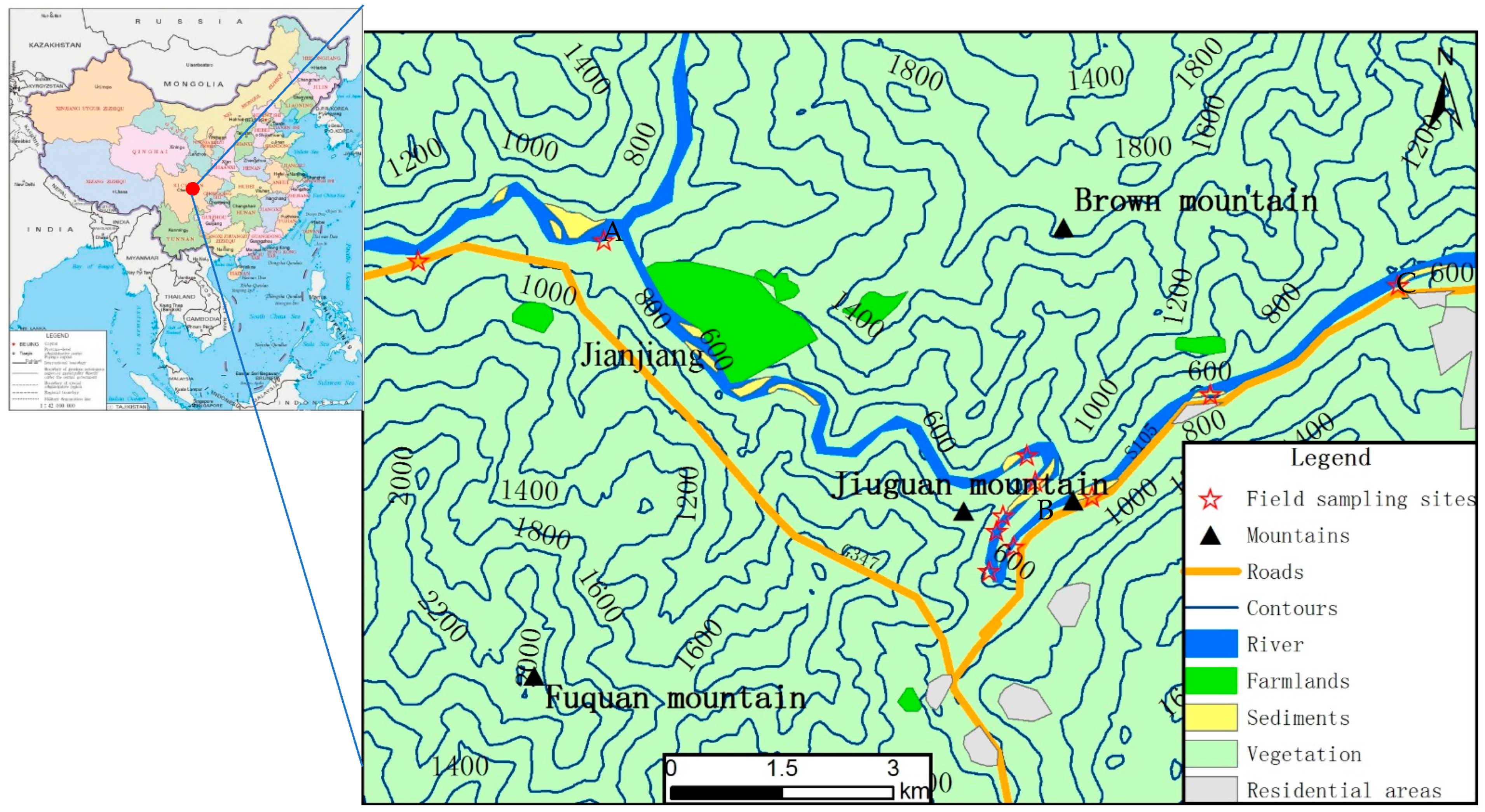
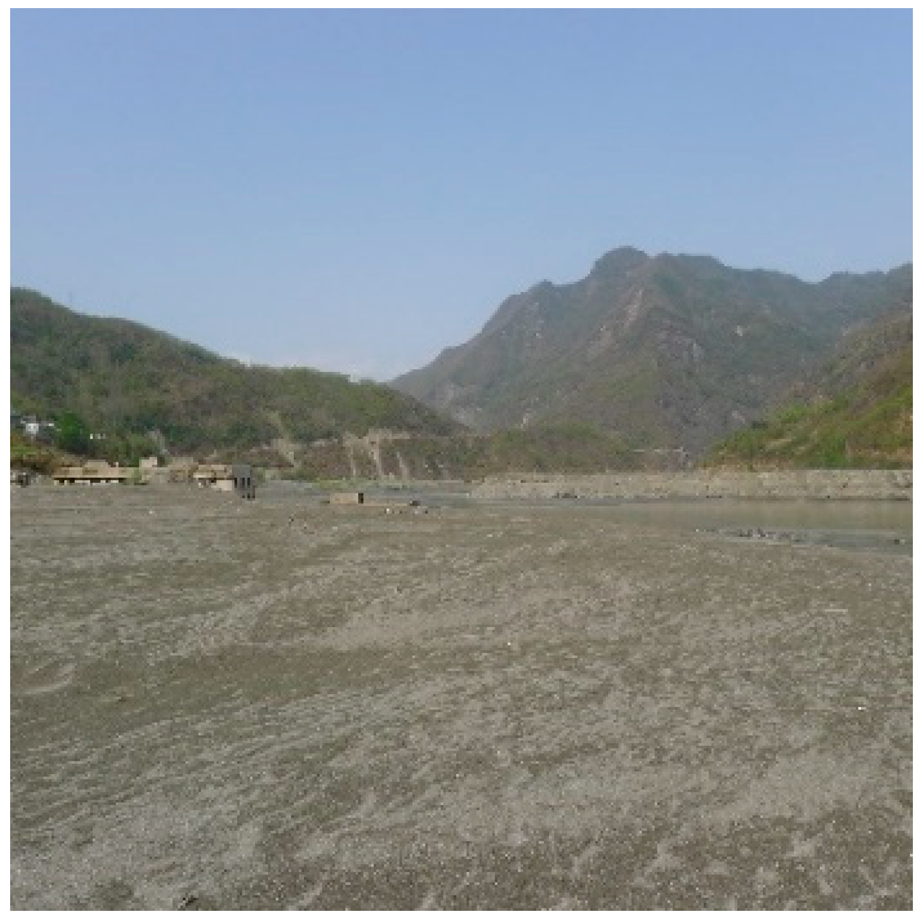
2.1. Study Area
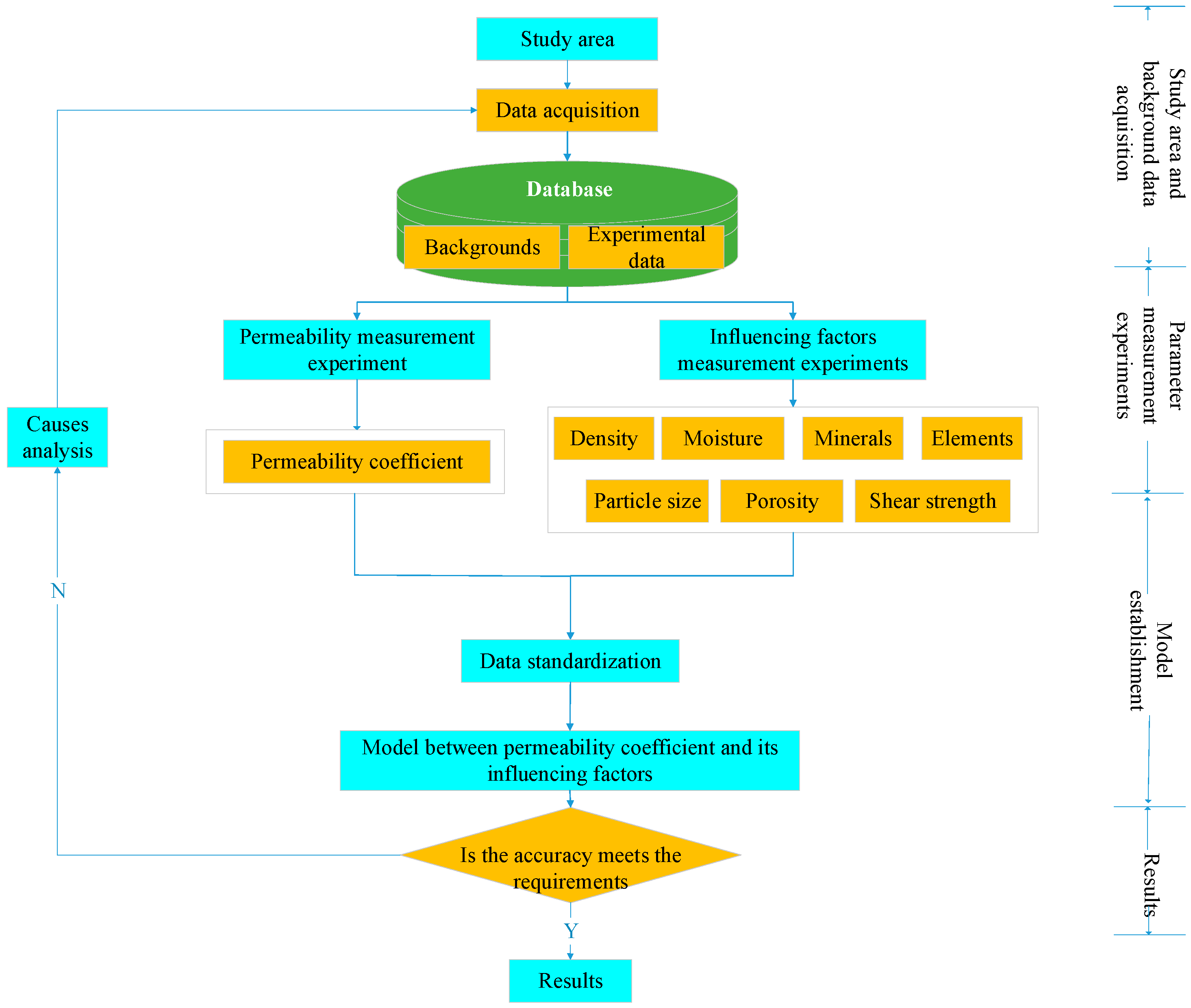
2.2. Methods
- (1)
- Study area and background data acquisition
- (2)
- Parameter measurement experiments
- (3)
- Model establishment
- (4)
- Results
2.3. Data Acquisition and Processing
2.3.1. Background Data
2.3.2. Samples
2.3.3. Parameter Measurement Experiments
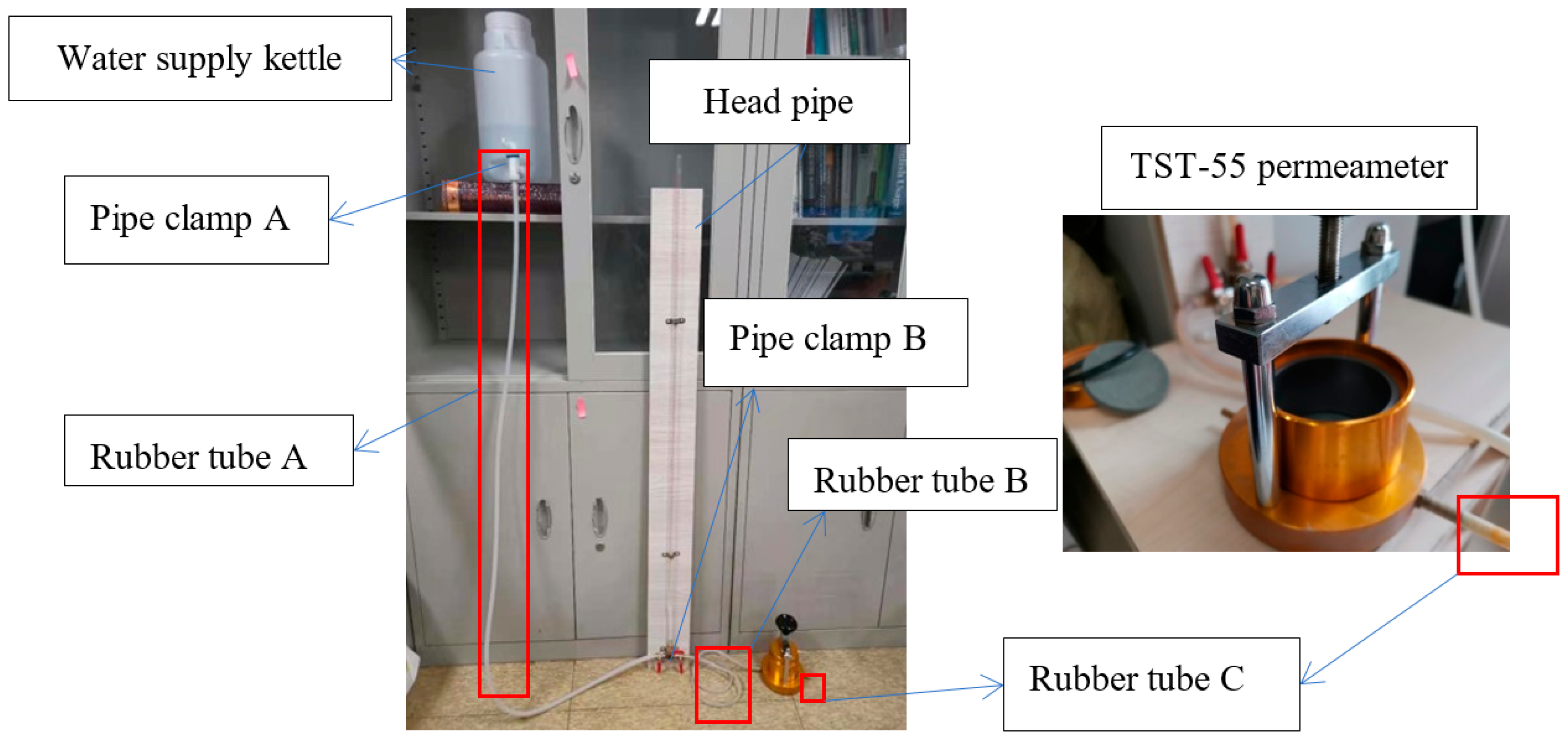
- (1)
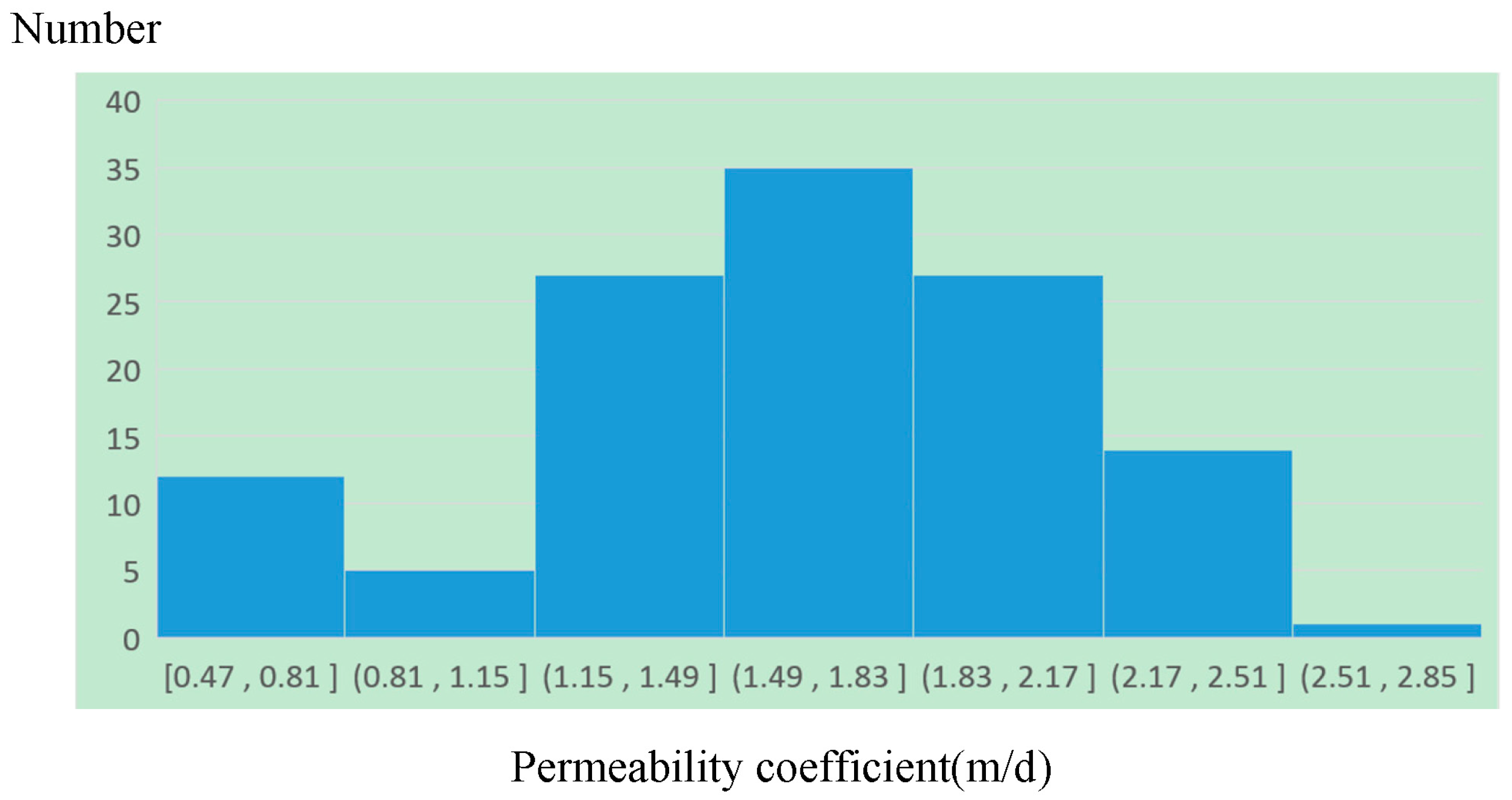
- Permeability coefficient measurement experiment
- (2)
- Measurement experiments on influencing factors of permeability coefficient
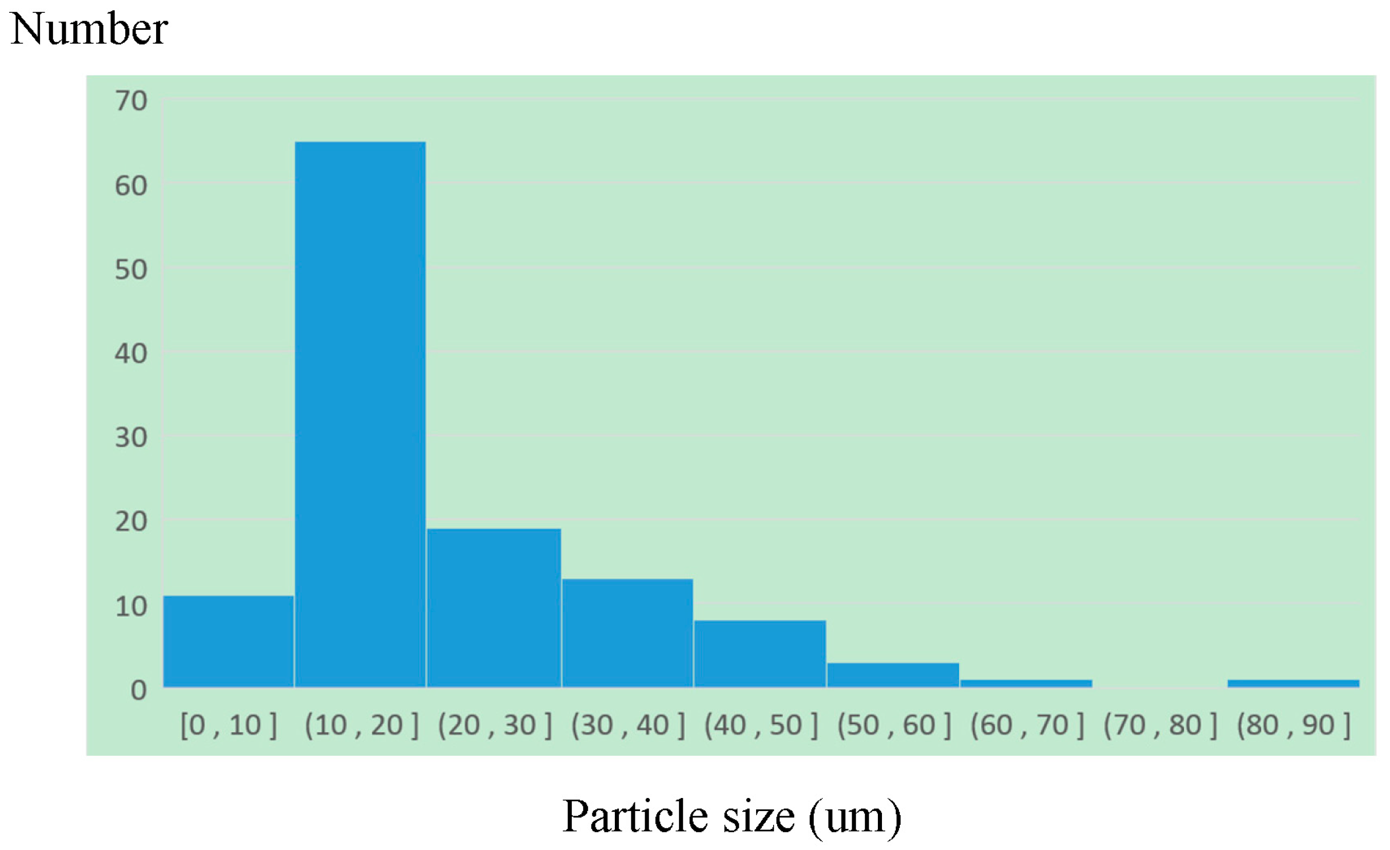
- (a)
- Particle size measurement experiment
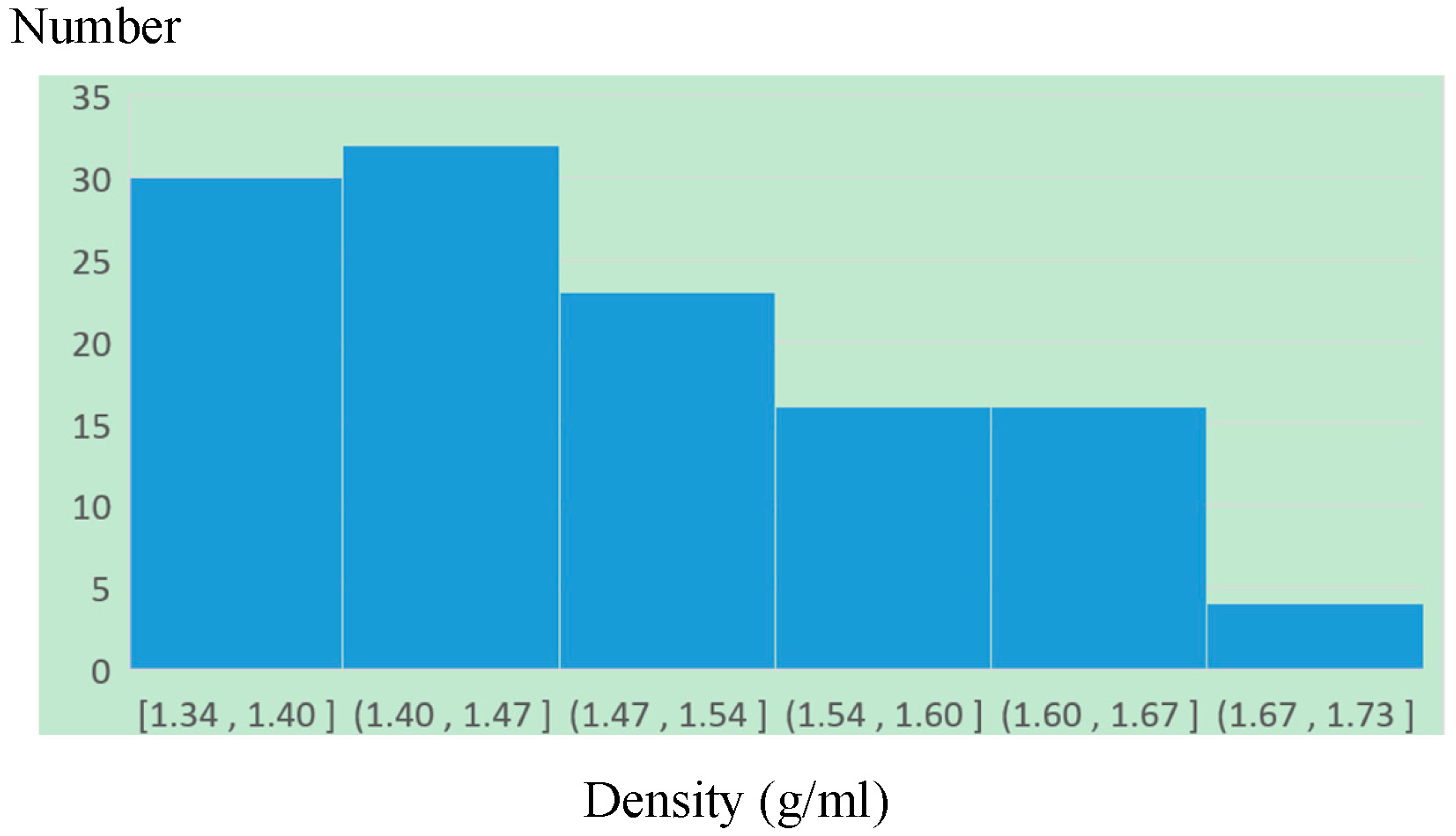
- (b)
- Density measurement experiment
- (c)
- Minerals measurement experiment
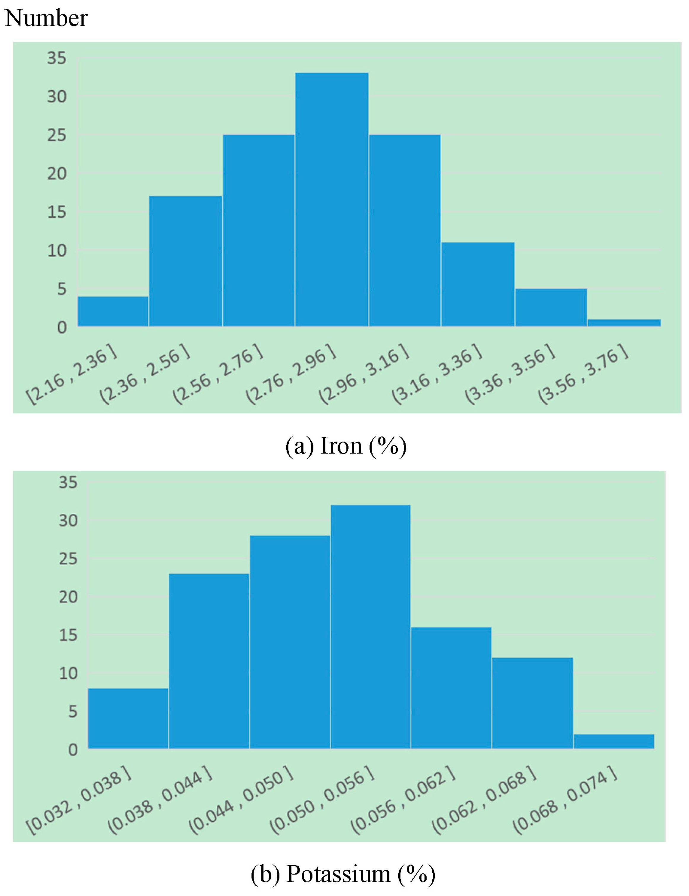
- (d)
- Element measurement experiment
- (e)
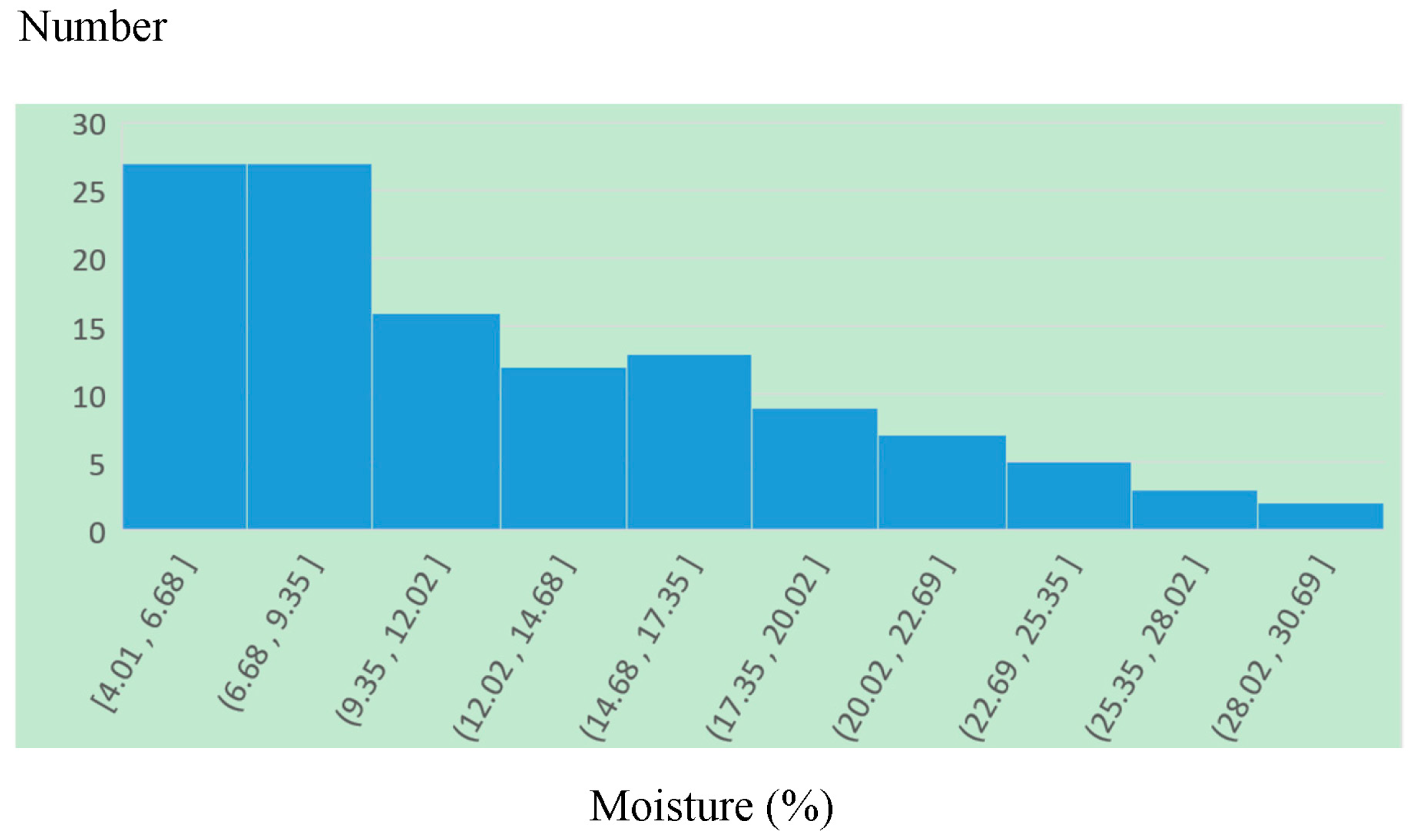
- Moisture measurement experiment
- (f)
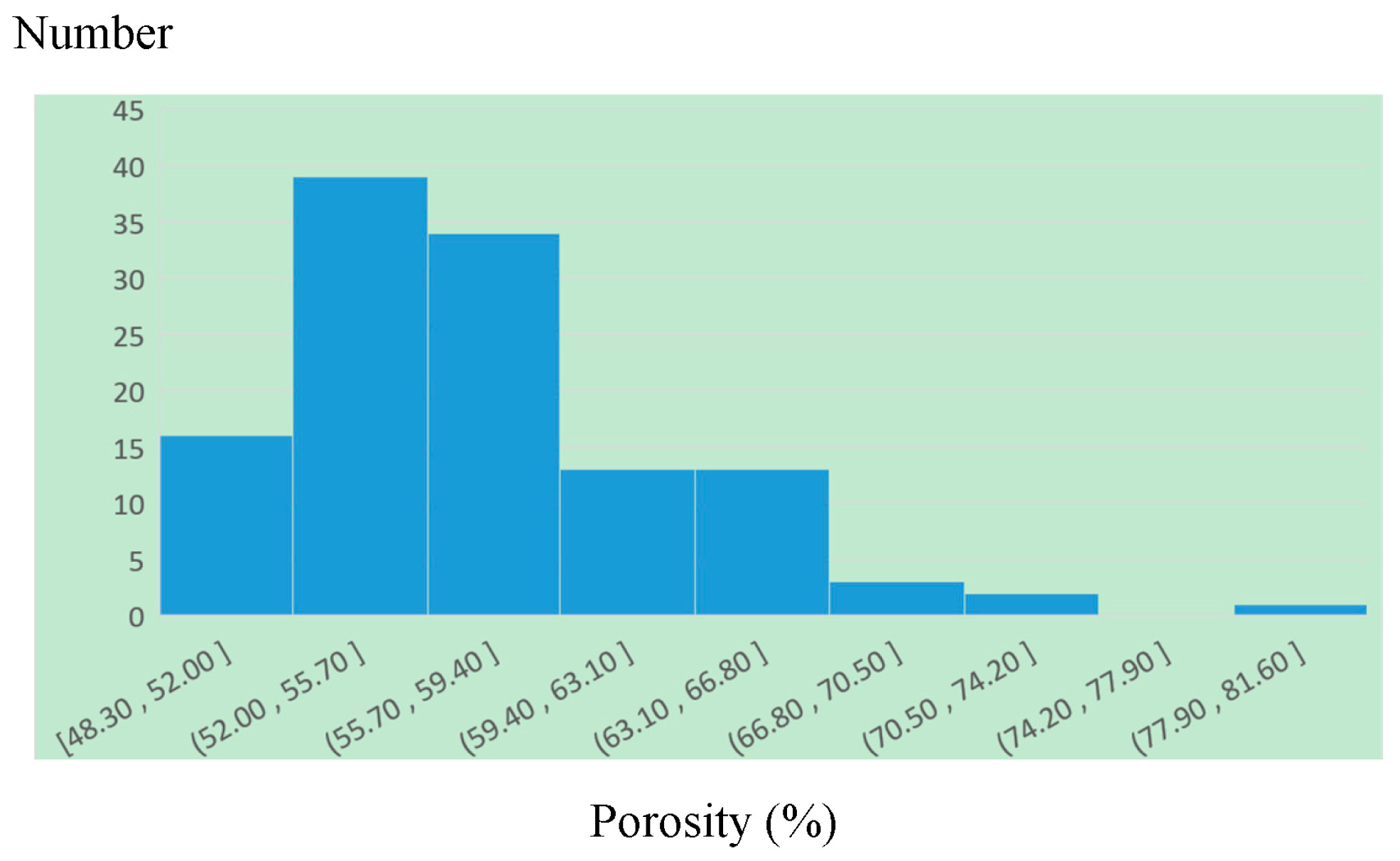
- Porosity measurement experiment
- (g)
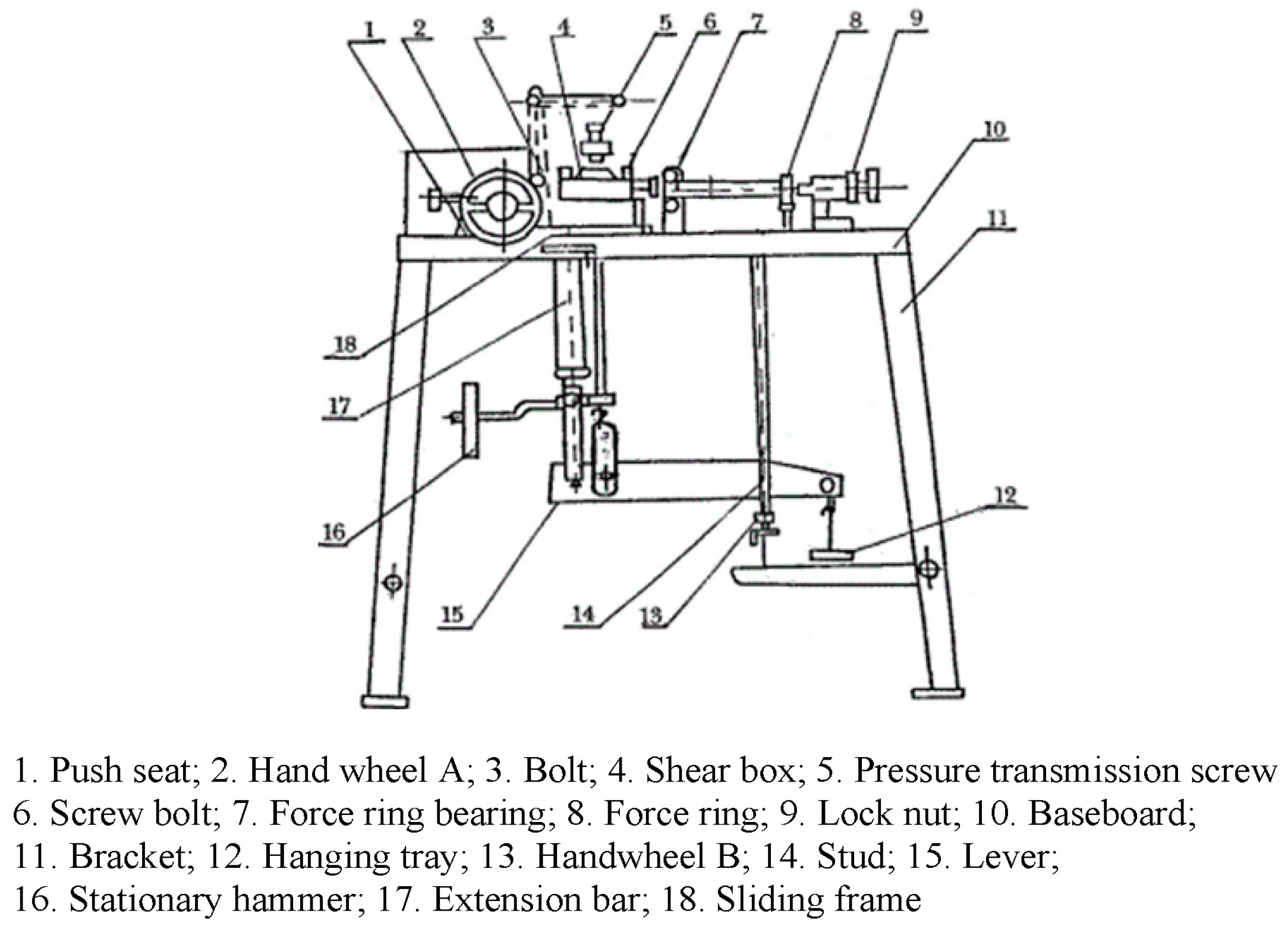
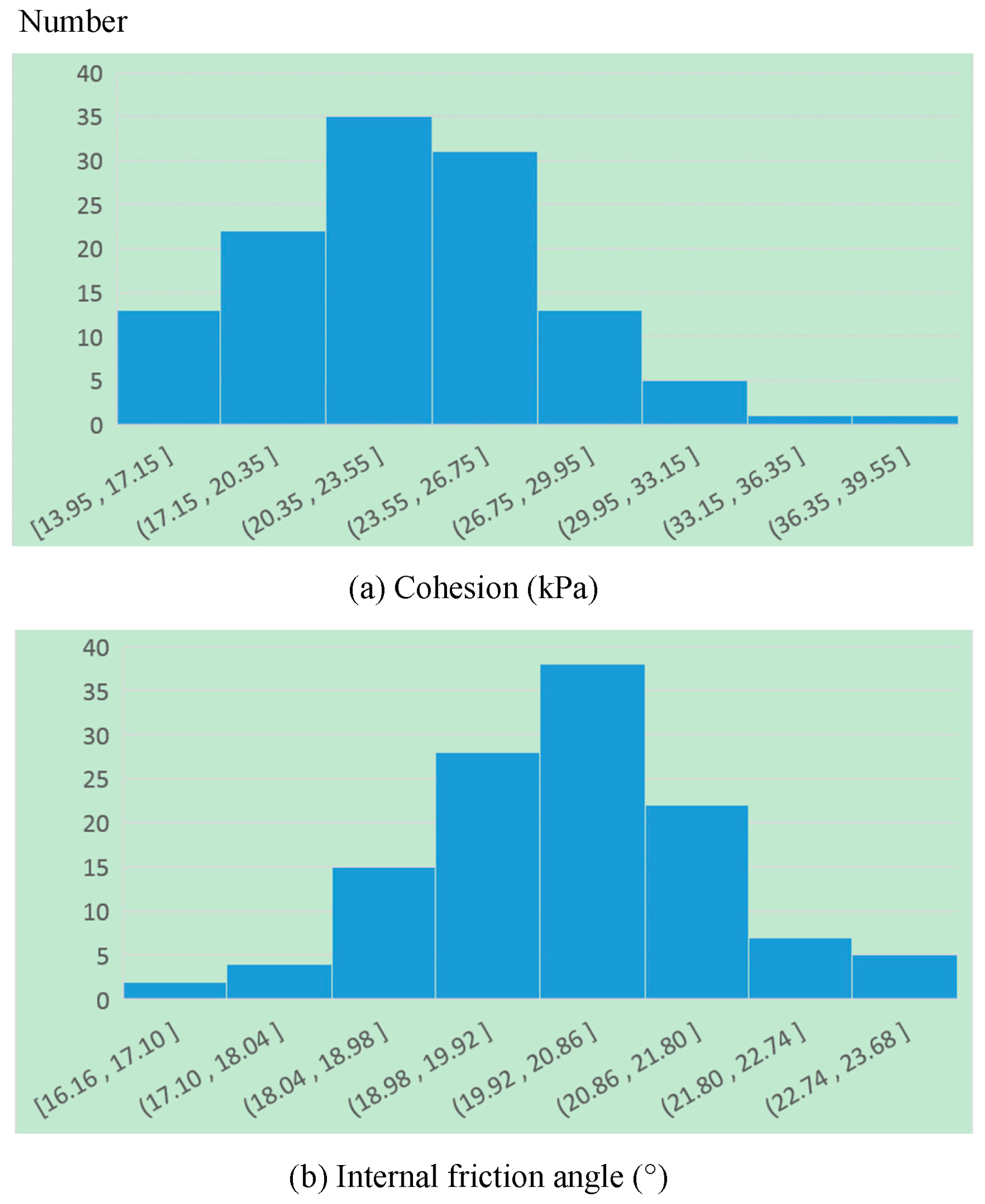
- Shear strength measurement experiment
2.3.4. Data Standardization
2.4. Model
- (1)
- Selection of sensitive factors
- (2)
- Multivariate regression analysis
3. Results
4. Discussion
5. Summary and Conclusions
Author Contributions
Funding
Institutional Review Board Statement
Informed Consent Statement
Data Availability Statement
Conflicts of Interest
References
- Liu, P.; Wei, Y.M.; Wang, Q.J.; Xie, J.J.; Chen, Y.; Li, Z.C.; Zhou, H.Y. A research on landslides automatic extraction model based on the improved mask R-CNN. ISPRS Int. J. Geo-Inf. 2021, 10, 168. [Google Scholar] [CrossRef]
- Xiao, J.B. The Emergency Management Department of China Announced the National Top Ten Disasters in 2019. Available online: http://society.people.com.cn/n1/2020/0112/c1008-31544517.html,2020 (accessed on 2 January 2022).
- Liu, D.Y.; Yu, K. Zhouqu: Why did “Longshang Jiangnan” become a muddy city. Land Resour. Guide 2010, 9, 20–21. [Google Scholar]
- Tang, C.; Liang, J.T. Study on characteristics of 9.24 rainstorm and debris flow in Beichuan, Wenchuan earthquake area. J. Eng. Geol. 2008, 16, 751–758. [Google Scholar]
- Wu, Q.; Xu, L.R.; Zhou, K.; Liu, Z.Q. Starting analysis of loose deposits of gully debris flow. J. Nat. Disasters 2015, 24, 89–97. [Google Scholar]
- Xu, X.C.; Chen, J.P.; Shan, B. Study of grain distribution characteristics of solid accumulation in debris flow. Yangtze River 2015, 46, 51–54. [Google Scholar]
- Ma, M. Stability analysis of high slope of accumulation at the outlet of pressure flood discharge and sediment discharge tunnel of Jiudianxia Water Control Project. Water Conserv. Plan. Des. 2019, 4, 64–67. [Google Scholar]
- Tang, M.G.; Xu, Q.; Li, J.Q.; Luo, J.; Kuang, Y. An experimental study of the failure mechanism of shallow landslides after earthquake triggered by rainfall. Hydrogeol. Eng. Geol. 2016, 43, 128–135. [Google Scholar]
- Jonathan, W.F.R.; Reuben, A.H.; Brian, S.I. Particle size distribution of main-channel-bed sediments along the upper Mississippi River, USA. Geomorphology 2016, 264, 118–131. [Google Scholar]
- Xie, J.; Wang, M.; Liu, K.; Coulthard, T.J. Modeling sediment movement and channel response to rainfall variability after a major earthquake. Geomorphology 2018, 320, 18–32. [Google Scholar] [CrossRef]
- Marcel, H.; Velio, C.; Coraline, B.; Guo, X.; Berti, M.; Graf, C.; Hübl, J.; Miyata, S.; Smith, J.B.; Yin, H.-Y. Debris-flow monitoring and warning: Review and examples. Earth-Sci. Rev. 2019, 199, 102981. [Google Scholar] [CrossRef]
- Dobrokhotov, V.; Oakes, L.; Sowell, D.; Larin, A.; Hall, J.; Kengne, A.; Bakharev, P.; Corti, G.; Cantrell, T.; Prakash, T.; et al. Toward the nanospring-based artificial olfactory system for trace-detection of flammable and explosive vapors. Sens. Actuators B Chem. 2012, 168, 138–148. [Google Scholar] [CrossRef]
- Philip, K.L.; Lalit, K.; Richard, K. Monitoring river channel dynamics using remote sensing and GIS techniques. Geomorphology 2019, 325, 92–102. [Google Scholar]
- Miao, Q.H.; Yang, D.W.; Yang, H.B.; Li, Z. Establishing a rainfall threshold for flash flood warnings in China’s mountainous areas based on a distributed hydrological model. J. Hydrol. 2016, 541, 371–386. [Google Scholar] [CrossRef]
- Wang, Q.J.; Wei, Y.M.; Chen, Y.; Lin, Q.Z. Hyperspectral Soil Dispersion Model for the Source Region of the Zhouqu Debris Flow, Gansu, China. IEEE J. Sel. Top. Appl. Earth Obs. Remote Sens. 2016, 9, 876–883. [Google Scholar] [CrossRef]
- Fan, R.L.; Zhang, L.M.; Wang, H.J.; Fan, X.M. Evolution of debris flow activities in Gaojiagou Ravine during 2008–2016 after the Wenchuan earthquake. Eng. Geol. 2018, 235, 1–10. [Google Scholar] [CrossRef]
- Hu, W.; Scaringi, G.; Xu, Q.; Pei, Z.; Van Asch, T.W.; Hicher, P.-Y. Sensitivity of the initiation and runout of flowslides in loose granular deposits to the content of small particles: An insight from flume tests. Eng. Geol. 2017, 231, 34–44. [Google Scholar] [CrossRef]
- Liu, Y. Study on test method of permeability coefficient of cohesionless coarse-grained soil in hydraulic engineering. Shanxi Water Conserv. 2020, 12, 211–213. [Google Scholar]
- Bayat, B.; Van, D.T.C.; Yang, P.Q.; Verhoef, W. Extending the SCOPE model to combine optical reflectance and soil moisture observations for remote sensing of ecosystem functioning under water stress conditions. Remote Sens. Environ. 2019, 221, 286–301. [Google Scholar] [CrossRef]
- Elżbieta, R.; Maciej, D.; Kazimierz, K. Sediment budget of high mountain stream channels in an arid zone (High Atlas mountains, Morocco). Catena 2020, 190, 104530. [Google Scholar] [CrossRef]
- Jiang, F.; Zhan, Z.; Chen, J.; Lin, J.; Wang, M.K.; Ge, H.; Huang, Y. Rill erosion processes on a steep colluvial deposit slope under heavy rainfall in flume experiments with artificial rain. Catena 2018, 169, 46–58. [Google Scholar] [CrossRef]
- Friedl, F.; Weitbrecht, V.; Robert, M.B. Erosion pattern of artificial gravel deposits. Int. J. Sediment Res. 2018, 33, 57–67. [Google Scholar] [CrossRef]
- Wei, J.; Shi, B.L.; Li, J.L.; Li, S.S.; He, X.B. Shear strength of purple soil bunds under different soil water contents and dry densities: A case study in the Three Gorges Reservoir Area, China. Catena 2018, 166, 124–133. [Google Scholar] [CrossRef]
- Lin, J.; Huang, Y.; Zhao, G.; Jiang, F.; Wang, M.-K.; Ge, H. Flow-driven soil erosion processes and the size selectivity of eroded sediment on steep slopes using colluvial deposits in a permanent gully. Catena 2017, 157, 47–57. [Google Scholar] [CrossRef]
- Li, M.W.; Tang, C.; Chen, M. Spatio-temporal evolution characteristics of landslides in debris flow catchment in Beichuan County in the Wenchuan earthquake zone. Hydrogeol. Eng. Geol. 2020, 47, 182–190. [Google Scholar]
- Li, C.X.; Ma, Y.; He, Y.X. Sensitivity analysis of debris flow to environmental factors: A case of Longxi River basin in Dujiangyan, Sichuan Province. Chin. J. Geol. Hazard Control 2020, 31, 32–39. [Google Scholar]
- Ye, L. The Relationship between the Distribution of Debris Flow and Environmental factors—A Case Study of Counties in Northern Mianyang City. J. Baoshan Univ. 2021, 40, 64–70. [Google Scholar]
- Yang, B.X.; Cao, D.J. The technology innovation and inspiration of “GF-2” satellite high-resolution camera. Spacecr. Recovery Remote Sens. 2015, 36, 10–15. [Google Scholar]
- Yin, Y.P.; Zhang, Z.C.; Zhang, M.S.; Zheng, W.M.; Wei, L.W.; Wu, S.R.; Zhang, R.S.; Yao, X.; Zhang, K.J.; Li, X.C.; et al. Geological and Mineral Industry Standard of the People’s Republic of China: Code for Investigation of Landslide, Collapse and Debris Flow Disasters 1:50,000 (DZ/T 02161-2014); China Standards Press: Beijing, China, 2015. [Google Scholar]
- Xu, M.; Yang, L.Z.; Wang, D.H.; Chen, M.J.; Chu, W.Y. National Standard of the People’s Republic of China: Technical Guide for Soil Sampling of Soil Quality (GB/T 36197-2018); China National Standardization Administration Committee: Beijing, China, 2018.
- Sheng, S.X.; Dou, Y.; Tao, X.Z.; Zhu, S.Z.; Xu, B.M.; Li, Q.Y.; Guo, X.L.; He, X.M. National Standard of the People’s Republic of China: Geotechnical Test Code (SL237-1999); China Water Resources and Hydropower Press: Beijing, China, 1999. [Google Scholar]
- Li, C.M.; Wang, D.; Liu, X.L.; Tan, M.J.; Liu, Y.; Jin, Z.G.; Yin, Y.; Wu, Y.J.; Qiu, R.Q.; Sun, W.; et al. National Standard of the People’s Republic of China: Basic Provisions for Basic Geographic Information Database (GB/T 30319-2013); China National Standardization Administration Committee: Beijing, China, 2013.
- Fan, M.Q.; Teng, Y.J.; Wu, W.; Liu, Y.H.; Luo, M.Y.; Wang, Y.; Xin, H.B.; Zhang, W.; Wen, Y.F.; Gong, B.W.; et al. Engineering Classification Standard for Soil (GB/T 50145-2007); China Planning Press: Beijing, China, 2008. [Google Scholar]
- Sun, X.D.; Wang, D. Analysis of cohesion value of soil. Liaon. Build. Mater. 2010, 3, 39–42. [Google Scholar]
- Zhang, X.J.; Liu, P.; Yang, X.Q.; Wang, Y. A Study of the Relationship between Permeability and Pore Structure of Lime-treated Loess. J. Guangdong Univ. Technol. 2021, 38, 97–105. [Google Scholar]
- Liu, H.W.; Dang, F.N.; Tian, W.; Mao, L.M. Prediction of permeability of clay by modified Kozeny—Carman equation. Chin. J. Geotech. Eng. 2021, 43 (Suppl. S1), 186–191. [Google Scholar]
- Fan, G.Y.; Zhang, J.M.; Shen, J.B. Laboratory study on penetration resistance of sandy soil modified in high sandy soil area. Shanxi Archit. 2021, 47, 68–70. [Google Scholar]
- Hou, Y.B.; Qiao, D.X. Influence of Compaction on Strength and Permeability of Total Tailings Consolidation Body. Met. Mine 2021, 10, 67–74. [Google Scholar]
- Charlotte, J.W.V.V.; Julia, G. Effect of compaction and soil moisture on the effective permeability of sands for use in methane oxidation systems. Waste Manag. 2020, 107, 44–53. [Google Scholar]
- Wang, S. Study on Seepage Law of Riverbed in Desert Section of Hotan River. Master’s Thesis, Tarim University, Xinjiang, China, 2021. [Google Scholar]
- Yu, J. Study on Permeability Characteristics and Fine Particle Migration Law of Deposited Soil in Debris Flow Channel. Master’s Thesis, Sichuan Normal University, Chengdu, China, 2020. [Google Scholar]

| Particle Size | Montmorillonite | K | Fe | Moisture | Density | Porosity | Permeability Coefficient (p) | ln(p) | Internal Friction Angle | Cohesion | |
|---|---|---|---|---|---|---|---|---|---|---|---|
| Particle size | 1.00 | −0.12 | −0.05 | −0.03 | 0.07 | 0.13 | −0.04 | 0.00 | 0.00 | −0.05 | 0.08 |
| Montmorillonite | −0.12 | 1.00 | −0.25 | −0.32 | 0.37 | 0.31 | 0.18 | 0.00 | −0.02 | −0.04 | −0.03 |
| K | −0.05 | −0.25 | 1.00 | 0.82 | −0.74 | −0.58 | −0.42 | 0.16 | 0.20 | −0.09 | −0.04 |
| Fe | −0.03 | −0.32 | 0.82 | 1.00 | −0.65 | −0.56 | −0.33 | 0.11 | 0.16 | −0.15 | −0.06 |
| Moisture | 0.07 | 0.37 | −0.74 | −0.65 | 1.00 | 0.80 | 0.70 | −0.43 | −0.48 | −0.13 | 0.32 |
| Density | 0.13 | 0.31 | −0.58 | −0.56 | 0.80 | 1.00 | 0.38 | −0.46 | −0.51 | −0.08 | 0.36 |
| Porosity | −0.04 | 0.18 | −0.42 | −0.33 | 0.70 | 0.38 | 1.00 | −0.46 | −0.51 | −0.10 | 0.29 |
| Permeability coefficient (p) | 0.00 | 0.00 | 0.16 | 0.11 | −0.43 | −0.46 | −0.46 | 1.00 | 0.97 | 0.32 | −0.56 |
| ln(p) | 0.00 | −0.02 | 0.20 | 0.16 | −0.48 | −0.51 | −0.51 | 0.97 | 1.00 | 0.31 | −0.58 |
| Internal friction angle | −0.05 | −0.04 | −0.09 | −0.15 | −0.13 | −0.08 | −0.10 | 0.32 | 0.31 | 1.00 | −0.66 |
| Cohesion | 0.08 | −0.03 | −0.04 | −0.06 | 0.32 | 0.36 | 0.29 | −0.56 | −0.58 | −0.66 | 1.00 |
| No. | Influencing Factors | Permeability Coefficient (p, m/d) | ln(p) (m/d) |
|---|---|---|---|
| 1 | Cohesion (kPa) | −0.55681 | −0.5834 |
| 2 | Porosity (%) | −0.46196 | −0.51413 |
| 3 | Density (g/mL) | −0.45947 | −0.51207 |
| 4 | Moisture (%) | −0.42836 | −0.4769 |
| 5 | Internal friction angle (°) | 0.323295 | 0.308409 |
| 6 | K (%) | 0.16128 | 0.195123 |
| 7 | Fe (%) | 0.113593 | 0.155239 |
| 8 | Montmorillonite (%) | 0.003181 | −0.01579 |
| 9 | Particle size (um) | 0.002364 | 0.0011 |
| Coefficient | p Value | Lower Limit 95% | Upper Limit 95% | |
|---|---|---|---|---|
| Intercept | 0.1875 | 6.53 × 10−38 | 0.16814 | 0.20687 |
| Density | −0.0387 | 0.00063 | −0.0605 | −0.01688 |
| Porosity | −0.0455 | 4.77 × 10⁻⁵ | −0.06679 | −0.02415 |
| Cohesion | −0.0619 | 5.44 × 10⁻⁸ | −0.08295 | −0.04079 |
Publisher’s Note: MDPI stays neutral with regard to jurisdictional claims in published maps and institutional affiliations. |
© 2022 by the authors. Licensee MDPI, Basel, Switzerland. This article is an open access article distributed under the terms and conditions of the Creative Commons Attribution (CC BY) license (https://creativecommons.org/licenses/by/4.0/).
Share and Cite
Wang, Q.; Xie, J.; Yang, J.; Liu, P.; Chang, D.; Xu, W. Research on Permeability Coefficient of Fine Sediments in Debris-Flow Gullies, Southwestern China. Soil Syst. 2022, 6, 29. https://doi.org/10.3390/soilsystems6010029
Wang Q, Xie J, Yang J, Liu P, Chang D, Xu W. Research on Permeability Coefficient of Fine Sediments in Debris-Flow Gullies, Southwestern China. Soil Systems. 2022; 6(1):29. https://doi.org/10.3390/soilsystems6010029
Chicago/Turabian StyleWang, Qinjun, Jingjing Xie, Jingyi Yang, Peng Liu, Dingkun Chang, and Wentao Xu. 2022. "Research on Permeability Coefficient of Fine Sediments in Debris-Flow Gullies, Southwestern China" Soil Systems 6, no. 1: 29. https://doi.org/10.3390/soilsystems6010029
APA StyleWang, Q., Xie, J., Yang, J., Liu, P., Chang, D., & Xu, W. (2022). Research on Permeability Coefficient of Fine Sediments in Debris-Flow Gullies, Southwestern China. Soil Systems, 6(1), 29. https://doi.org/10.3390/soilsystems6010029