Comparative Assessment of Digital and Conventional Soil Mapping: A Case Study of the Southern Cis-Ural Region, Russia

Abstract

Digital mapping was applied for a key site located at the Southern Cis-Ural region near Ufa city (the Republic of Bashkortostan, Russia). The digital soil map (DSM) was created using the open-source GIS software packages and compared to a conventional (CSM) one. As input parameters, we used standard morphometric values of the topography and field descriptions of soils, including the authors’ data. The DSM was created at the same scale (1:25,000) as the CSM, and soils of different classes were grouped according to the principle of genetic homogeneity and regional agroecological value. Comparing DSM and CSM showed several significant differences in the position, areas, and boundaries of hydromorphic soils and chernozems. The DSM has advantages over CSM at estimating smaller soil areas (areals) and their boundaries, in particular, on elevated topography elements (hills and steep slopes) and upper links of the erosion network (small dry valleys, hollows, and gullies). On the other hand, fluvial soils are mapped rather poorly by the digital approach, and CSM is more appropriate for such soils’ areals. The highest discrepancy is confined to the areas of eroded soils and fluvisols (15% and 12% of total area, respectively) due to significant differences in DSM and CSM approaches for such soil groups. We suppose that the digital method is effective and suitable for the Cis-Ural region, despite 57% soil taxa (types) prediction accuracy and the complexity of the territory by its ruggedness, erosion, and suffusion processes. The implementation and further use of digital mapping methods increase the quality of work, reduce its cost and terms in the region.

1. Introduction

Modern soil mapping combines traditional/conventional (visual-expert) and digital methods. In recent decades, the worldwide growing interest in digital soil maps/mapping (DSM) has been accompanied by a downward trend in the use of conventional maps/mapping (CSM) [1]. Comparative assessments of CSM and DSM are few, while the “real data” of digital mapping and the “conceptual assumptions” of conventional ones, of course, are not compared in favor of the latter [2]. Today’s mood and tendency in soil mapping suppose that DSM preferences are mainly related to: (1) the decrease in subjective (expert) opinion, making maps more objective and reproducible [3]; (2) the reduction of the cost of the mapping process [4,5,6,7,8]; (3) increasing the informativeness of soil maps [9,10]; (4) creating a global DSM [1,11].

Soil mapping in Russia has deep traditions. Mapping methods are primarily inherited from the soil–landscape paradigm of V.V. Dokuchaev. Despite the significant development of the DSM globally, soil maps in Russia were created mainly based on conventional approaches due to the history of domestic soil geography. The first attempts at “soil mapping” in Russia were undertaken back in the 15th century. Mainly, information about soils was collected for the purpose of taxing peasants. The methods of studying soils were primitive, without a detailed analysis of the soil cover. The main criterion for soil assessment was its fertility. “Black” lands were considered as fertile, and “white” or “whitish”—unproductive. Mass soil mapping began in the 1930s–1950s when collective and state farms were formed in the USSR. This was caused by the need to carry out of following tasks: the formation of a land management plan and substantiation of agrochemical measures, reclamation of saline and waterlogged soils, irrigation planning in arid regions, and developing new areas. Over a couple of decades, large and medium-scale soil maps were created for the most of Russian agricultural territories. These maps were made using the conventional (i.e., generally accepted) method [12].

In the 1970s–1980s, the CSM had changed somewhat. This was due to computerization, applying remote sensing data and developing new soil mapping concepts. For example, the Russian soil-cartographic school is associated with the concept of soil cover structure (SCS) [13]. According to this doctrine, the SCS has a hierarchical organization, and depending on the study scale/area; different units serve as the object of mapping. Instead of one dominant soil unit, some maps showed the so-called soil combinations—two to four genetically related soil units. On large-scale maps, these combinations of two to four soil types are due to meso-relief elements. The reflection of accompanying components in each cartographic unit increased the information content of maps for inventory, monitoring, and rational use of soil cover. In particular, the mapping of soil combinations turned out to be in demand for practical purposes since it turned out to be vastly convenient for agriculture.

Today, the DSM in Russia is developing [3,14,15,16,17], but not very intensively compared to foreign countries [6,11,18,19]. However, all results/studies concur about the advantage of using GIS technologies for large and medium-scale DSM. In Russia, conventional and digital approaches still compete; thus, it is essential to compare them. In particular, a comparison of the results of CSM and DSM in the relatively logically deterministic landscape conditions of the Central Russian Upland (Belgorod Oblast) did not reveal fundamental differences in the total areas and spatial arrangement of soils of different taxa, but showed differences in the area of soils with varying erosion intensity. In the case of CSM use, a significant (by three–four times) underestimation of the areas of moderately and strongly eroded soils is noted, because of the poor consideration for factors other than slope steepness in the development of erosion-accumulative processes. With an increase in the steepness of slopes, the discrepancies between the assessments of soil eroded area obtained by CSM and DSM methods tend to increase [17]. The authors are unaware of works using DSM methods alone or comparing with CSM for the Cis-Ural region.

This study aimed to compare the results of CSM and DSM in contrasting landscapes with a predominance of complex micro- and meso-reliefs, high variability of parent rocks, and land use. Such lands include, as a rule, foothill territories. This study selected a key site in the Cis-Ural region in European Russia (in the Republic of Bashkortostan—RB) (Figure 1a,b).

2. Objects and Methods

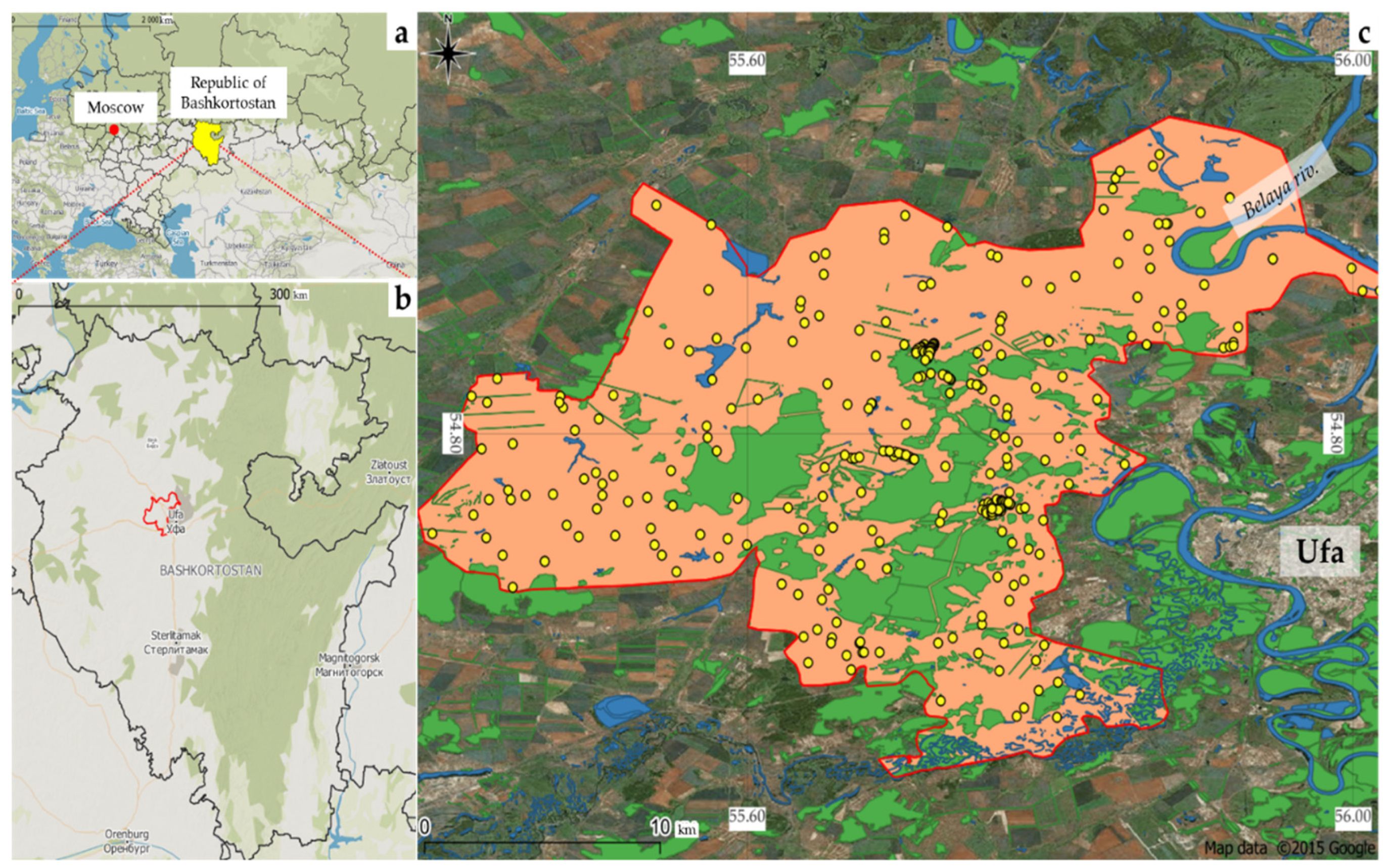
2.1. Study Site Description

The study site (~51,830 ha) is located within the Ufa district of the RB (Figure 1b,c), in the Pribelskaya hilly plain, 100 km west of the macroslope of the South Urals ridge. The hydrographic network of this region is represented by the Belaya River and its tributaries: Ufa, Urshak, and Dyoma rivers. The geographical position, particularly the abundance of floodplain areas and uplands, resulted in an intense dissection of the relief. At the same time, most of the territory of the study site involved the agrarian sector (Figure 1c). For example, among agricultural land (70% of the total area in the Ufa district) only, more than 42% is located on slopes with a steepness of 1–5° [20]. However, it is known that for agriculture, first of all, the territories where the relief is the least dissected are allotted. The climate within the study area is temperate continental, relatively humid (Dfb according to the Köppen–Geiger climate classification [21]). The annual average air temperature is +3.8 °C. Selyaninov’s hydrothermal coefficient (HTC) [22] of humidification is 1.0–1.2 (i.e., slightly humid). The average annual precipitation is 589 mm, about 2/3 of which falls in the summer [23]. The frequency of rainfall with an intensity of 5–7 mm/min does not exceed 5%. The work [24] shows that at such intensity, surface runoff and soil washout begin as early as 5–7 min from the onset of rainfall, and the soil loss reaches 50–100 t/ha, depending on soil type and slope inclination. For the development of erosion processes, an intensity of falling drops of more than 2 mm/min is sufficient, which refers to rains in the category of “showers”. The frequency of such rainfall in the Ufa district is 37.3% of the annual total precipitations; it determines the development of rainfall erosion during the vegetation season. Winter in the region is moderately cold and long. The period with a stable snow cover lasts on average about 5.5 months (from November to April); the average snowpack depth is 0.5 m. The depth of soil freezing reaches 94 cm [25], which, combined with other agro-climatic factors, contributes to soil erosion during snowmelt [26]. Broad-leaved forests with an admixture of birch and oak are widespread in the region Wind erosion is minimal in the study region despite the low forest cover [27].

Along with developing water-erosion processes in the region, karst formation also occurs. In the RB, about 50% of the territory is subject to suffusion processes; almost 30% of them are affected by surface karst manifestations. Dozens of new karst sinkholes are recorded annually; abnormally large sinkholes with a diameter of more than 15 m and a depth of >10 m occur once every 5–6 years [28]. Thus, the forest-steppe zone of the Cis-Urals and, in particular, the Ufa district of the RB are characterized by meso- and micro-relief, the formation of which is due to the complex impact of various exogenous processes. Such processes and the dissected relief of the Ufa district complicate soil mapping (both CSM and DSM).

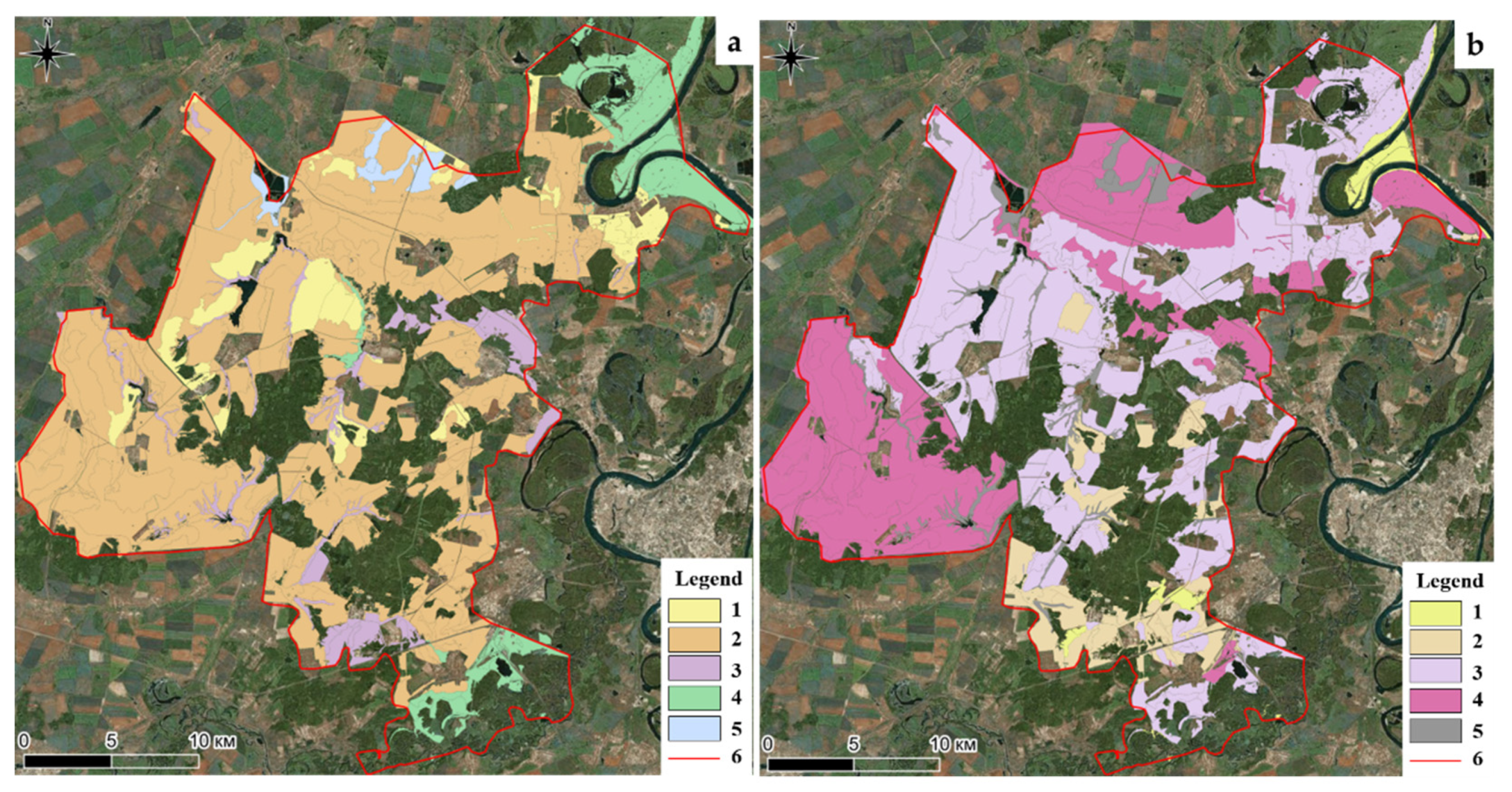
2.2. CSM and Field Data Processing

For the RB, a comprehensive field survey and creation of soil maps were carried out in the 1970s–1980s. Almost 50 years later, updating maps and the monitoring of soils in the RB began again. In 2016, soil scientists of the Bashkir State Agrarian University (BSAU) carried out work on field soil survey, digitization and creation/correction of electronic soil maps, and the formation of explications of soil varieties and agricultural land [29]. The existing soil maps in the RB were created by the conventional method with a 1:25,000 scale. For DSM creation, we used the existing CSM (of 2016) and our own data. The soil sampling array (soil profiles) included 367 descriptions (Figure 1c) with a georeferencing accuracy of up to 10 m, taken from CSM (312 descriptions) and completed during our field survey (55 descriptions). All soil profile locations were chosen in a way to cover the maximum number of different topography forms and soil types. The description of soil profiles (e.g., morphological properties, texture, and soil type determination) was carried out in situ by visual-expert and tactile methods and then refined based on laboratory analysis.

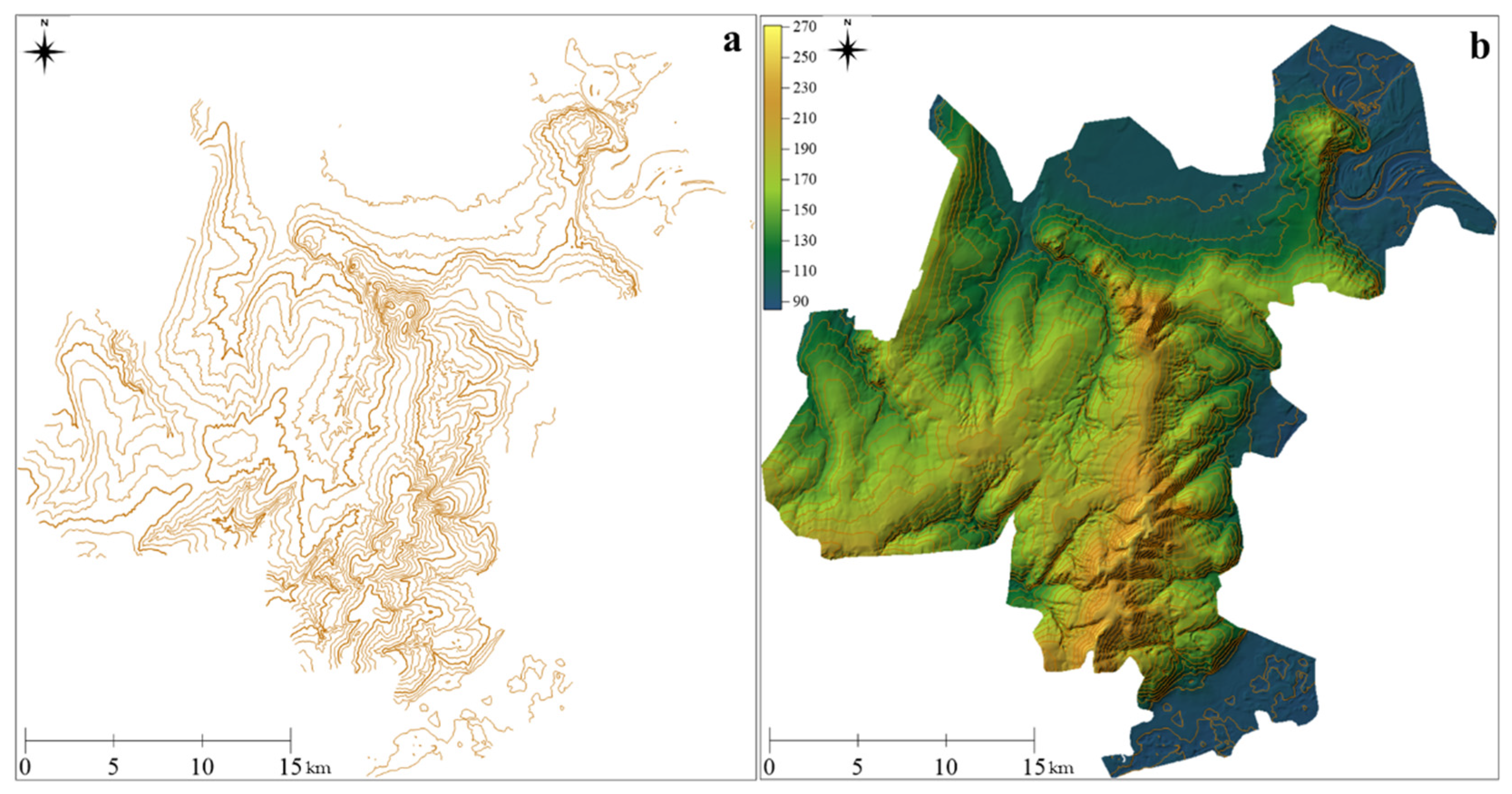
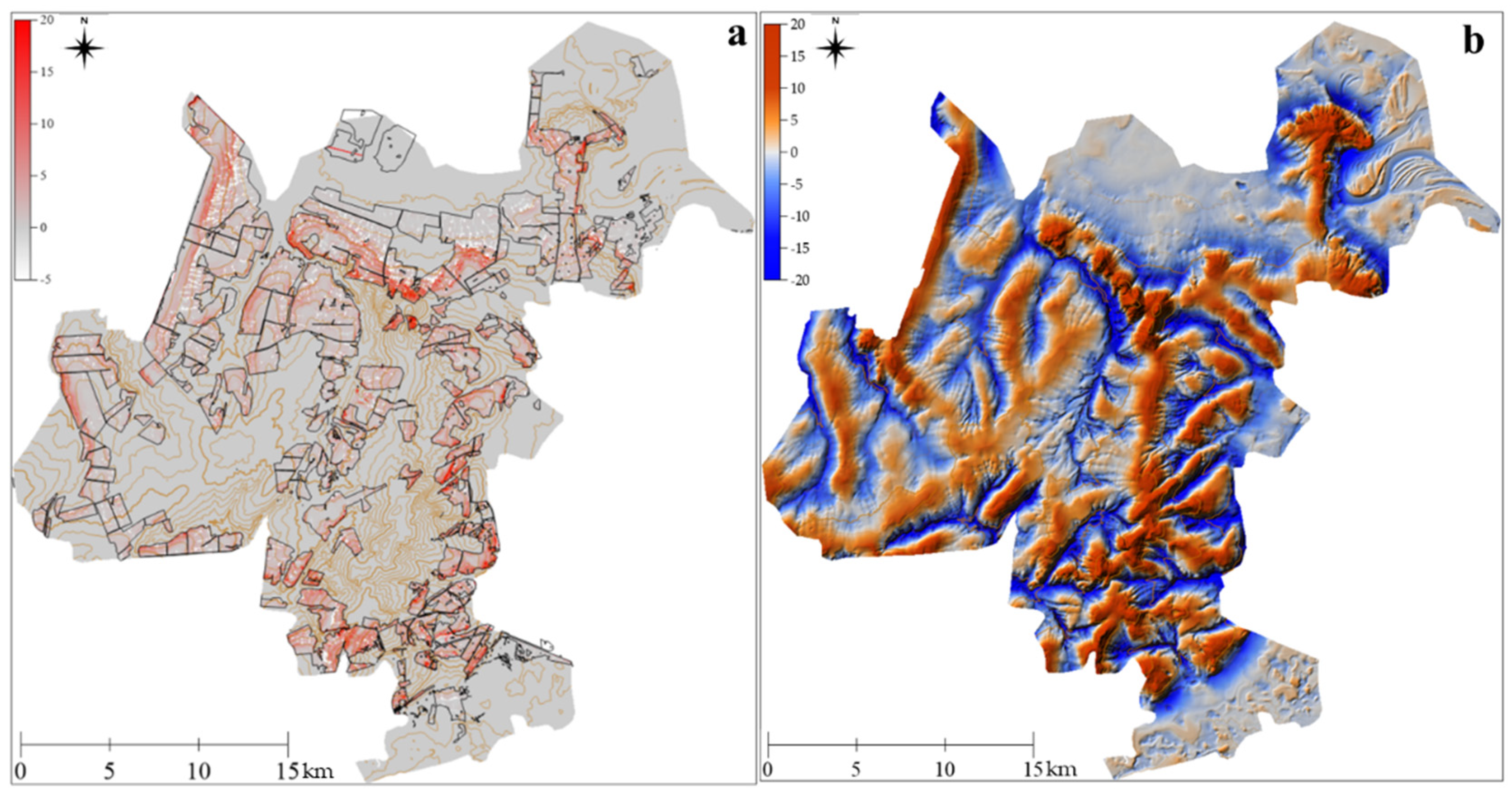
2.3. DSM Methodology

The relief and character of sediments/parent material are the leading factors in soil cover differentiation [20,30,31]. The parent material (Figure 2a) and soil texture (Figure 2b) of the study area are typical for the region. The dominant textures of the topsoil (horizon A) are loam and clay formed on eluvial and deluvial loams.

To improve the quality of creating a digital elevation model (DEM), it is desirable to use large-scale topographic maps, the availability of which in the public domain in most cases is limited. We used detailed topographic maps with a basic cross-section of 2.5 m contour lines in this work. Based on these maps, the contour lines (Figure 3a) were digitized in the QGIS program, and the DEM (Figure 3b) was built in the SAGA GIS program [32] with a resolution of 20 × 20 m by the ordinary kriging method. The scale of DSM was set at 1:25,000 (the same as in CSM). Moreover, the program calculated more than 20 morphometric values reflecting the redistribution processes of heat and moisture [33]. It should be noted that considering the detail of the original topographic maps and the pixel size of the DEM 20 × 20 m, the morphometric values characterize the state of the earth’s surface with dimensions of at least 60 × 60 m elementary soil structures [13,34].

The canonical discriminant analysis was used to model soil–landscape relationships [35,36]. It allows ranking topographic factors according to their contribution to explaining the spatial variability of soil classes and calculating the posterior probability of a pixel’s soil belonging to each soil class following the normal distribution function. The subsequent analysis of the posterior probabilities makes it possible to obtain for each pixel: (1) the certainty of the forecast, as the value of the maximum probability of all possible; (2) the most probable class of soils. The results were verified by comparing the observed and predicted soil taxa at description points.

Areas of eroded soils were also identified by a digital method based on data from a field survey of soils and a mathematical erosion model WaTEM/SEDEM. In particular, the model was applied to determine soil loss/accumulation rates and detection of areas/areals affected by water erosion. The following input parameters were used in the model: (1) data on the rainfall erosivity factor (R-factor) are equal to 240–265 MJ·mm·ha⁻²·h⁻¹·yr⁻¹ according to [37]; (2) the values of erodibility of chernozems (K-factor) were 35 kg·h·MJ⁻¹·mm⁻¹; (3) the soil-protective role (C-factor) of cultivated crops in the crop rotation relative to the erodibility of pure fallow is set at 0.37 [38]. As a result of applying the WaTEM/SEDEM model, soil erosion rates were obtained (Figure 4a) for each cell of the regular grid. The maximum erosion intensity within the key site reaches 20 t/ha per year and is comparable with the data obtained using other methods.

By overlaying the field sampling points on a map of soil erosion rates, a table was obtained containing information on the degree and rates of soil erosion at each point. For each gradation of the calculated rates of erosion (0–5, 5–10, 10–15, etc. t/ha per year), the proportion of soils with different degrees of erosion intensity was calculated. Empirical functions were used to detect the degree of soil erosion in a pixel according to the method described in [39]. Pixels with a total probability of participation of weakly, moderately, and strongly eroded soils of more than 50% were assigned to the category of eroded soils.

3. Results and Discussion

The soil cover within the study area is heterogeneous and diverse. Field survey revealed the following types/subtypes of soils according to the WRB [40]: haplic and luvic chernozems (loamic, hyperhumic, pachic), eutric arenosols (aric, humic), greyzemic stagnic chernic phaeozems (loamic, hyperhumic, pachic), greyzemic gleyic chernic phaeozems (loamic, hyperhumic, pachic), luvic stagnic chernic phaeozems (loamic, hyperhumic, pachic), fluvisols, peat soils, and soils’ complexes of hollows and small dry valleys. According to the principle of genetic homogeneity and agroecological value, the soils were grouped into soil classes/groups: automorphic (all chernozem soils), lithogenic (some arenosols), semi-hydromorphic (stagnic phaeozems), medium- and waterlogged (gleyic phaeozems and other waterlogged soils), floodplain (fluvisols) as well as eroded soils without taxa separation (Figure 5). Chernozems, phaeosems, and fluvisols are usually characterized by a loam and clay texture and arenosols are mostly sandy–loamy (Figure 2b). The regional specific in the particle size distribution of soils lies in the fact that sandy and sandy–loamy soils are widespread within the high interfluves. These areas are not used and not suitable for crop cultivation for the following reasons: lack of nutrients and available water, the spread of erosion processes and/or partial afforestation.

From the broad set of morphometric relief values, the following variables were significant in the separation of soil groups in the attribute space (

Table 1. Significance of variables in soil taxa/group description.

Terrain Parameter	Fisher’s Criterion	p-Value	Physical Sense
Intercept	29.1	0.0
Topographic wetness index	17.0	0.0	Separates soils of an increasing range of moisture as moisture accumulates in concave relief elements
Channel network base level	15.6	0.0	Determines the position of sandy stagnic soils within the high interfluves
Relative slope position	20.1	0.0
Topographic position index	16.0	0.0	Separates soils of convex and concave landforms

): topographic wetness index [41], channel network base level [42], relative slope position [42] and topographic position index (Figure 4b) with radius 1500 m [41].

The discriminant analysis total accuracy was about 57% (

Table 2. Prediction accuracy of soil groups in the study site.

No. and Color of Soil Group	WRB Index	Accuracy, %	Predicted Soils, Units
			Ch	Ar	St Ph	Fl	Gl Ph
1	Ch	69	138	24	1	8	11
2	Ar	50	17	22	1	1	3
3	St Ph	35	2	1	6	7	1
4	Fl	72	0	0	4	15	2
5	Gl Ph	42	2	1	0	4	5
	General	57	200	53	12	35	24

Note: The description of WRB indexes (codes), numbers and colors of soil groups are given in Figure 5.

) in predicting the position of soil taxa in the directive and territorial space. This indicates the possibility of using DSM in areas with complex relief and subject to erosion and suffusion processes in the case of using detailed DEM. It should be noted that there are factors that reduce the model’s reliability. This is due, first of all, to the overlap of some soil taxa in the attribute space and possible errors in binding the points of field descriptions.

The final map of soil groups (Figure 5) reveals with acceptable accuracy the main features of the structure and diversity of the soil cover of the study area, where the dominant soil types are combinations of typical and leached chernozems. Semi-hydromorphic and hydromorphic soils with an increasing range of moisture were formed in wide, slightly concave hollows and small dry valleys. Phaeozems soils occupy the upper parts of hollows. The middle and lower parts of hollows and plumes of slopes with significant extra moisture are occupied by phaeozems soils. The disadvantage of the presented model is the low quality of predicting the areas of hydromorphic (including floodplain) soils, which largely overlap in the feature space of the variables used.

The DSM also shows the regional features of the soil cover. In particular, the position of arenosols in the most convex parts of the high interfluves of the Pribelskaya Upland is clearly distinguished. These soils were formed on sandy loams and sands and have a very thin or almost absent cover of loess-like loams.

Eroded soils, their distribution, and areas are also characterized by regional-specific features. It is generally accepted that erosional SCS have a “tree-like” distribution pattern [13]. A methodology similar to the one used in this work for mapping eroded soils in the Kursk and Belgorod oblasts of European Russia indicated the presence of such a “tree-like” image of soil erosion patterns within the Central Russian Upland [17,39]. However, in the study area in the RB, the classical “tree-like” structure of erosional SCS does not appear, which is probably due to the originality (ruggedness) of the terrain. This feature was noted by us earlier in the field survey and conventional mapping of erosion-accumulation microstructures of the soil cover at the key site within the Ufa district of the RB [43].

The CSM results (Figure 6) were combined to similar groups as it was completed for DSM.

For a more convenient comparison of DSM and CSM, we show fragments of soil maps in the central part of the study site (Figure 7). There are some differences in the presented maps. First of all, the shape of areas of soil groups is somewhat different. Due to well-detailed topography data, the DSM is better in concave positions on hill slopes. On the other hand, the alluvial soils are better shown on a CSM. The DSM shows large areas of hydromorphic soils, but not alluvial, that are typical for floodplains. This is a lack of used predictors in DSM. Space images and Quaternary maps were used to obtain better forecasting results. Secondly, the areas of eroded soils differ significantly. Based on erosion modelling, the DSM approach shows high prediction/detalization of eroded soil areas. For conventional mapping methodology, eroded soil patterns are determined based on slope steepness and cannot show the same detail.

The presented maps differ in soil groups’ areas (

Table 3. The share of soil groups.

No. and Color of Soil Group	WRB Index	DSM		CSM		Area Difference, ha
		Area, ha	%	Area, ha	%
1	Ch	22,286	43	20,732	40	1554
2	Ar	2690	5	3628	7	938
3	St Ph	2802	5	5701	11	2899
4	Fl	8246	16	2073	4	6173
5	Gl Ph	9896	19	6220	12	3676
6	Er	5910	11	13,476	26	7566
Total		51,830

Note: The WRB indexes (codes), numbers, and colors of soil groups are described in Figure 5.

). The dominant soil group for both maps is chernozems. They are related to the well-drained positions on the hills. The subdominant soil group for DSM is hydromorphic, and for CSM is eroded. These differences were described earlier, as well as for the alluvial soils of the floodplains. The most significant differences in areas are devoted to a group of eroded soils. Moreover, there are significant differences in areas of stagnic phaeozems. They are typical for concave topography forms, hollows, and small dry valleys. Their area on the DSM is twice more than the conventional one, due to using a topographic wetness index predictor in the model that was not completed during CSM.

Thus, the comparison of DSM and CSM on the example of different geomorphological areas of the study site (in particular, river valley and watershed slopes, complicated by a network of hollows and small dry valleys) showed that DSM is not inferior to CSM methods, and in some cases shows an even more complete and a realistic pattern of the distribution of some soil types and their boundaries.

The DSM for a part of the Ufa district of the RB has a high potential and can be used for the agroecological assessment of lands and intra-field differentiation of agro-technologies.

4. Conclusions

The digital soil mapping (DSM) methodology was tested at one of the key sites of the Ufa district, the Republic of Bashkortostan (RB). It is shown that this method is effective for mapping the soil cover within the territories complicated by erosion and suffusion processes and having a complex terrain in the case of using detailed digital elevation models. Significant advantages of using the DSM compared to the conventional soil mapping (CSM) were revealed. Firstly, the DSM is a quantitative rather than a subjective approach. Secondly, the resulting DSM shows the shape, size, and position of the areas of eroded soils and shows hydromorphic soils in concave topography forms in much more detail.

On the other hand, the CSM created by specialists using detailed topography and soil data is devoid of potential errors associated with the imperfection of input data. The comparison showed a high difference in areas of soil groups; it is desirable to carry out the additional field soil sampling for better verification and DSM improvement. The highest discrepancy is confined to the areas of eroded soils and fluvisols (15% and 12% of total area, respectively) due to significant differences in DSM and CSM approaches for such soil groups and the high complexity of the topography. It was previously noted in [17] that the discrepancies are much more minor under less complex microrelief conditions. In this case, the subjective expert assessment underlying the traditional mapping doubled the area of eroded soils. On the other hand, based on the analysis of only the relief, the approach used is not entirely correct for floodplain soils areas. This can be eliminated by improving the composition of the predictors, including geological and space images data.

Today’s realities have forced us to assay DSM methods for the RB. Due to high topography and geological complexity, such methods have not previously been used in the region. The experience gained in this work can be used and projected for other territories with a similar specific karst-erosion relief. The use of DSM methods allows the reduction of the cost and speeding up of the work process. It also makes it possible to create more objective (based on formalized parameters) maps, but requires a large number of environmental covariates compared to conventional mapping methodology. The DSM results have increasing importance and high potential in precision agriculture. The authors would like to note that the CSM is by no means a poor method; it has high quality and accuracy. The CSM and DSM are two different products created in two different ways, each with its own advantages and disadvantages.

References

1. Nikiforova, A.A.; Fleis, M.E.; Nyrtsov, M.V.; Kazantsev, N.N.; Kim, K.V.; Belyonova, N.K.; Kim, J.K. Problems of modern soil mapping and ways to solve them. Catena 2020, 195, 104885. [Google Scholar] [CrossRef]
2. Hartemink, A.E.; Krasilnikov, P.; Bockheim, J.G. Soil maps of the world. Geoderma 2013, 207–208, 256–267. [Google Scholar] [CrossRef]
3. Kozlov, D.N.; Sorokina, N.P. Tradition and innovation in large-scale soil mapping. In Digital Soil Mapping: Theoretical and Experimental Research; V.V. Dokuchaev Soil Science Institute: Moscow, Russia, 2012; pp. 35–57. (In Russian) [Google Scholar]
4. Baruck, J.; Nestroy, O.; Sartori, G.; Baize, D.; Traidl, R.; Vrščaj, B.; Bräm, E.; Gruber, F.E.; Heinrich, K.; Geitner, C. Soil classification and mapping in the Alps: The current state and future challenges. Geoderma 2016, 264, 312–331. [Google Scholar] [CrossRef]
5. Hartemink, A.E.; Hempel, J.; Lagacherie, P.; McBratney, A.B.; McKenzie, N.J. GlobalSoilMap.net—A New Digital Soil Map of the World. In Digital Soil Mapping. Bridging Research, Environmental Application, and Operation; Boettinger, J.L., Howell, D.W., Moore, A.C., Hartemink, A.E., Kienast-Brown, S., Eds.; Springer: Dordrecht, The Netherlands, 2010; pp. 423–428. [Google Scholar]
6. McBratney, A.B.; Mendonça Santos, M.L.; Minasny, B. On Digital Soil Mapping. Geoderma 2003, 117, 3–52. [Google Scholar] [CrossRef]
7. Omuto, C.; Nachtergaele, F.; Rojas, R.V. State of the Art Report on Global and Regional Soil Information: Where Are We? Where To Go? Food and Agriculture Organization of the United Nations: Rome, Italy, 2013; ISSN 9251074496. [Google Scholar]
8. Sanchez, P.A.; Ahamed, S.; Carré, F.; Hartemink, A.E.; Hempel, J.; Huising, J.; Lagacherie, P.; McBratney, A.B.; McKenzie, N.J.; Mendonça-Santos, M.L.; et al. Digital Soil Map of the World. Science 2009, 325, 680–681. [Google Scholar] [CrossRef] [PubMed] [Green Version]
9. Brevik, E.C.; Calzolari, C.; Miller, B.A.; Pereira, P.; Kabala, C.; Baumgarten, A.; Jordán, A. Soil mapping, classification, and pedologic modeling: History and future directions. Geoderma 2016, 264, 256–274. [Google Scholar] [CrossRef]
10. Regmi, N.R.; Rasmussen, C. Predictive mapping of soil-landscape relationships in the arid Southwest United States. Catena 2018, 165, 473–486. [Google Scholar] [CrossRef]
11. Arrouays, D.; Poggio, L.; Salazar Guerrero, O.A.; Mulder, V.L. Digital soil mapping and GlobalSoilMap. Main advances and ways forward. Geoderma Reg. 2020, 21, e00265. [Google Scholar] [CrossRef]
12. Shershukova, G.A. Development stages of the large-scale mapping of soils in the USSR. In Large-Scale Soil Mapping; Grigoriev, G.I., Ed.; Science: Moscow, Russia, 1971; pp. 144–166. (In Russian) [Google Scholar]
13. Fridland, V.M. Pattern of the Soil Cover; John Wiley & Sons: Hoboken, NJ, USA, 1977; ISBN 978-0470991671. [Google Scholar]
14. Khitrov, N.; Smirnova, M.; Lozbenev, N.; Levchenko, E.; Gribov, V.; Kozlov, D.; Rukhovich, D.; Kalinina, N.; Koroleva, P. The soil cover patterns of forest-steppe and steppe zones at the East-European Plain. Soil Sci. Annu. 2019, 70, 198–210. [Google Scholar] [CrossRef]
15. Koshelev, A.V. Digital mapping of soils with the use of SRTM data. In Bulletin of the Lower Volga Agro-University Complex: Science and Higher Professional Education; Volgograd State Agrarian University: Volgograd, Russia, 2018; Volume 52, pp. 159–166, (In Russian). [Google Scholar] [CrossRef]
16. Savin, I.Y.; Ovechkin, S.V. On the updating of medium-scale soil maps. Eurasian Soil Sci. 2014, 47, 987–994. [Google Scholar] [CrossRef]
17. Zhidkin, A.P.; Smirnova, M.A.; Gennadiev, A.N.; Lukin, S.V.; Zazdravnykh, Y.A.; Lozbenev, N.I. Digital Mapping of Soil Associations and Eroded Soils (Prokhorovskii District, Belgorod Oblast). Eurasian Soil Sci. 2021, 54, 13–24. [Google Scholar] [CrossRef]
18. Arrouays, D.; Richer-De-Forges, A.C.; Héliès, F.; Mulder, V.L.; Saby, N.P.; Chen, S.; Martin, M.P.; Dobarco, M.R.; Follain, S.; Jolivet, C.; et al. Impacts of national scale digital soil mapping programs in France. Geoderma Reg. 2020, 23, e00337. [Google Scholar] [CrossRef]
19. Minasny, B.; McBratney, A.B. Digital soil mapping: A brief history and some lessons. Geoderma 2016, 264, 301–311. [Google Scholar] [CrossRef]
20. Gabbasova, I.M.; Khabirov, I.K. Distribution, typology and assessing degraded soils of Bashkortostan. Vestn. Bashkir State Agrar. Univ. 2010, 2, 3–11. (In Russian) [Google Scholar]
21. Peel, M.C.; Finlayson, B.L.; McMahon, T.A. Updated world map of the Köppen-Geiger climate classification. Hydrol. Earth Syst. Sci. 2007, 11, 1633–1644. [Google Scholar] [CrossRef] [Green Version]
22. Selyaninov, G.L. About the agricultural evaluation of the climate. Trudy GGO 1928, 20, 177–185. (In Russian) [Google Scholar]
23. Abdrakhmanov, R.F.; Batanov, B.N.; Gabbasova, I.M.; Komissarov, A.V.; Maslov, V.V.; Yunusov, S.A. Water Balance Station; BSAU: Ufa, Russia, 2002; p. 82. (In Russian) [Google Scholar]
24. Sobol, N.V.; Gabbasova, I.M.; Komissarov, M.A. Effect of rainfall intensity and slope steepness on the development of soil erosion in the Southern Cis-Ural region (A model experiment). Eurasian Soil Sci. 2017, 50, 1098–1104. [Google Scholar] [CrossRef]
25. Khalevitskaya, G.S.; Babkina, M.I.; Kuznetsova, V.V. Agroclimatic Resources of the Bashkir ASSR; Gidrometeoizdat: Leningrad, Russia, 1976; p. 235. (In Russian) [Google Scholar]
26. Komissarov, M.A.; Gabbasova, I.M. Snowmelt-induced soil erosion on gentle slopes in the southern Cis-Ural region. Eurasian Soil Sci. 2014, 47, 598–607. [Google Scholar] [CrossRef]
27. Sobol, N.V.; Gabbasova, I.M.; Komissarov, M.A. Impact of climate changes on erosion processes in Republic of Bashkortostan. Arid Ecosyst. 2015, 5, 216–221. [Google Scholar] [CrossRef]
28. Smirnov, A.I.; Durnaeva, V.N.; Abdrakhmanov, R.F. GIS-technologies in study of geohazards of the southern Urals and Cis-Urals. Geol. Bull. 2018, 137–143. [Google Scholar] [CrossRef]
29. Khasanov, A.N. The Current State of Soil Fertility in Agricultural Landscapes of the Southern Forest-Steppe of the Republic of Bashkortostan. Ph.D. Thesis, Bashkir State Agrarian University, Ufa, Russia, 4 October 2019. (In Russian). [Google Scholar]
30. Bugaets, A.N.; Pshenichnikova, N.F.; Tereshkina, A.A.; Krasnopeev, S.M.; Gartsman, B.I. Analysis of the spatial differentiation of the soil cover in the south of the Far East of Russia by the example of the Komarovka River basin. Eurasian Soil Sci. 2015, 48, 231–239. [Google Scholar] [CrossRef]
31. Khaziev, F.K. Soils of Bashkortostan. Vol. 1. Ecologic-Genetic and Agroproductive Characterization; Gilem: Ufa, Russia, 1995; p. 385. (In Russian) [Google Scholar]
32. Conrad, O.; Bechtel, B.; Bock, M.; Dietrich, H.; Fischer, E.; Gerlitz, L.; Wehberg, J.; Wichmann, V.; Böhner, J. System for automated geoscientific analyses (SAGA) v. 2.1.4. Geosci. Model Dev. 2015, 8, 1991–2007. [Google Scholar] [CrossRef] [Green Version]
33. Florinsky, I.V. Digital Terrain Analysis in Soil Science and Geology; Academic Press: Amsterdam, The Netherlands, 2016; p. 506. [Google Scholar]
34. Hole, F.D.; Campbell, J.B. Soil Landscape Analysis; Rowman and Littlefield: Lanham, MD, USA, 1985; p. 214. ISBN 978-0865981409. [Google Scholar]
35. Puzachenko, Y.G. Mathematical Methods in Environmental and Geographic Research; Academy: Moscow, Russia, 2004; p. 416. (In Russian) [Google Scholar]
36. Webster, R.; Burrough, P.A. Multiple discriminant analysis in soil survey. Eur. J. Soil Sci. 1974, 25, 120–134. [Google Scholar] [CrossRef]
37. Panagos, P.; Borrelli, P.; Meusburger, K.; Yu, B.; Klik, A.; Lim, K.J.; Yang, J.E.; Ni, J.; Miao, C.; Chattopadhyay, N. Global rainfall erosivity assessment based on high-temporal resolution rainfall records. Sci. Rep. 2017, 7, 4175. [Google Scholar] [CrossRef] [PubMed] [Green Version]
38. Larionov, G.A. Soil Erosion and Deflation: Basic Patterns and Quantitative Estimates; Moscow University Publishing House: Moscow, Russia, 1993; p. 200. (In Russian) [Google Scholar]
39. Kozlov, D.N.; Zhidkin, A.P.; Lozbenev, N.I. Digital Mapping of Soil Cover Eroded Patterns on the Basis of Soil Erosion Simulation Model (Northern Forest-Steppe of the Central Russian Upland); V.V. Dokuchaev Soil Science Institute: Moscow, Russia, 2019; Volume 100, pp. 5–35, (In Russian). [Google Scholar] [CrossRef]
40. IUSS Working Group WRB. World Reference Base for Soil Resources 2014, update 2015. International soil classification system for naming soils and creating legends for soil maps. In World Soil Resources Reports; FAO: Rome, Italy, 2015; p. 182. [Google Scholar]
41. Weiss, A. Topographic position and landforms analysis. In Proceedings of the Poster Presentation, ESRI User Conference, San Diego, CA, USA, 9–13 July 2001; Volume 200. [Google Scholar]
42. Olaya, V.; Conrad, O. Geomorphometry in SAGA. Dev. Soil Sci. 2009, 33, 293–308. [Google Scholar] [CrossRef]
43. Zhidkin, A.P.; Komissarov, M.A. Erosion and accumulation microstructures of soil cover in the forest-steppe zone of the Cis-Urals, the Republic of Bashkortostan. Vestn. Bashkir State Agrar. Univ. 2020, 53, 12–20. (In Russian) [Google Scholar] [CrossRef]
Figure 1. Location of: (a) the RB (filled by yellow color) within European Russia; (b) the study site (its border is shown by a red line, as well in (c)) within the RB; (c) the study site and the location of soil sampling points (yellow circles) within the Ufa district; land use/cover map specification (gray color indicates urban areas, green—forest and park areas, orange—agricultural lands, blue—water bodies).
Soilsystems 06 00014 g001
Figure 2. The parent rocks (soil horizon C) of the study area: 1—alluvial (river terraces) deposits, 2—eluvial–deluvial carbonate loams, 3—eluvial–deluvial carbonate-free loams, 4—alluvial (floodplain) deposits, 5—lacustrine deposits, 6—the study site boundary (a); (b) Soil texture of the topsoil (horizon A): 1—sandy loam, 2—loam, 3—clay loam, 4—clay, 5—undivided deposits of hollows and small dry valleys, 6—the study site boundary.
Soilsystems 06 00014 g002
Figure 3. Digitized contours (a) and DEM, m (b) of the study area.
Soilsystems 06 00014 g003
Figure 4. The calculated intensity of soil losses (in red) and sedimentation (in grey), t/ha per year (a); the topographic position index map (b).
Soilsystems 06 00014 g004
Figure 5. The soil types/groups at the study site, obtained by the DSM method. 1—Chernozems (Ch); 2—Arenosols (Ar); 3—Stagnic Phaeozems (St Ph); 4—Fluvisols (Fl); 5—Gleyic Phaeozems and other waterlogged soils (Gl Ph); 6—eroded soils (Er); 7—the study site boundary.
Soilsystems 06 00014 g005
Figure 6. Soil groups at the study site, created by the CSM method. Note: The legend description is the same as in Figure 5.
Soilsystems 06 00014 g006
Figure 7. Soil groups of the study site, created by the DSM (a) and CSM (b) methods. Note: The numbers from 1 to 7 in the legend are the same as in Figure 5, while 8—absolute heights of isolines, 9—soil profiles location.
Soilsystems 06 00014 g007