
Ensemble Modeling on Near-Infrared Spectra as Rapid Tool for Assessment of Soil Health Indicators for Sustainable Food Production Systems

 , , , , and
Abstract
:1. Introduction
2. Materials and Methods
2.1. Soil Samples and Types
2.2. NIR Spectroscopy and Reference Laboratory Analysis
2.3. NIR Ensemble Modeling Using Spectroscopic Data
2.4. Model Validation
2.5. Statistical Analysis
3. Results
3.1. Soil Properties across the Study Sites and Spectral Datasets
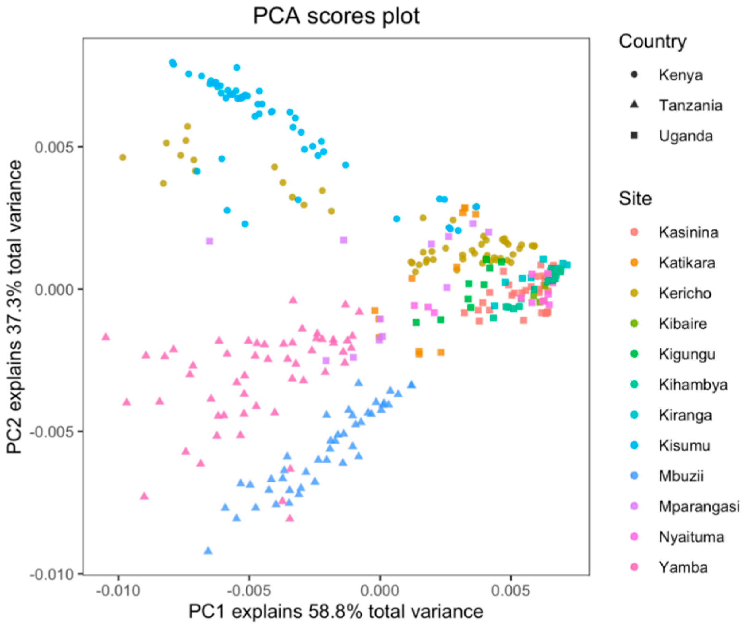
3.2. Exploratory Analysis of Soils Near-Infrared Spectra
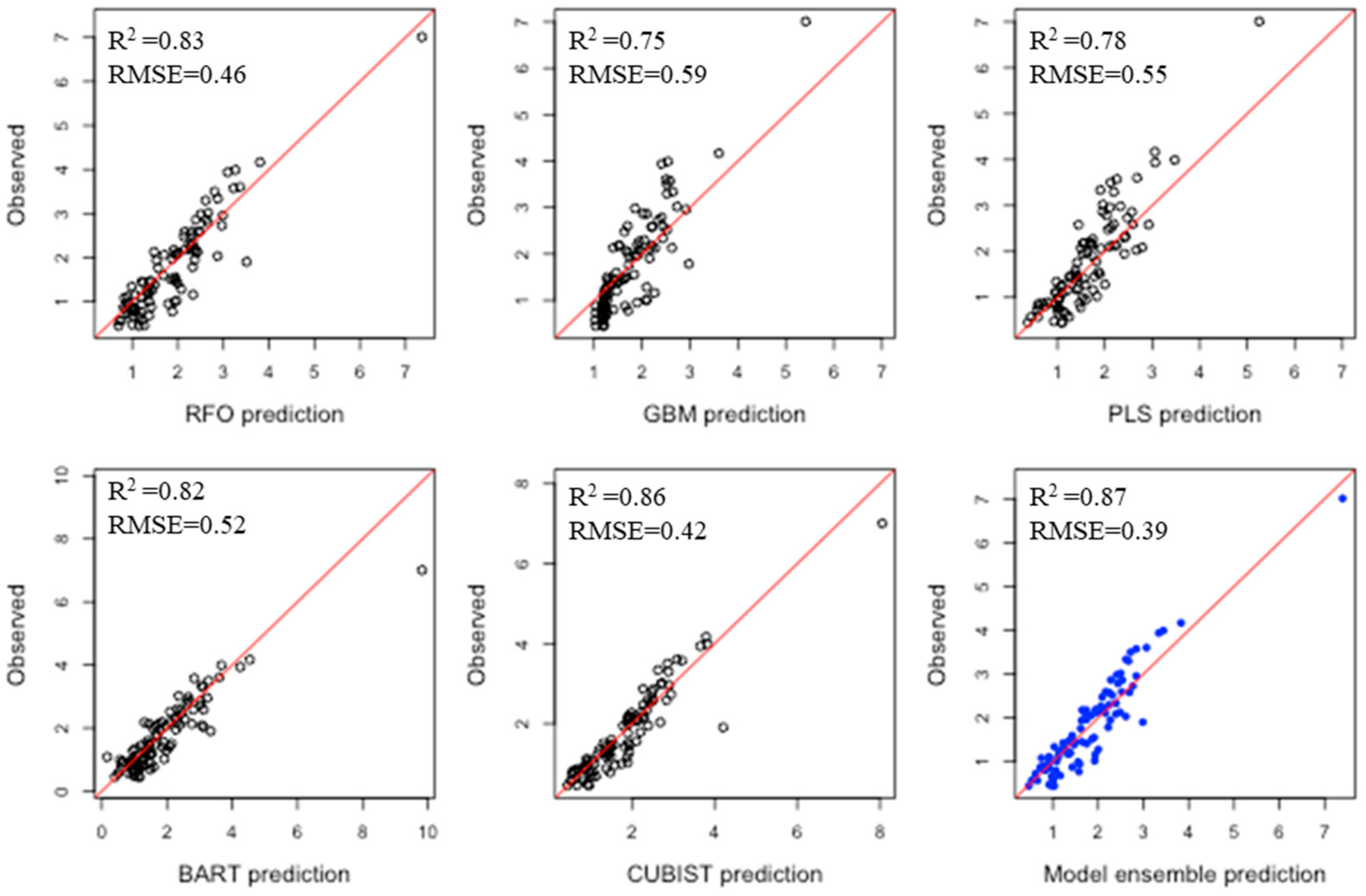
3.3. Comparison of Machine Learning Algorithms for Prediction of Soil Properties
3.4. Soil Health Indicators of Different Land Uses as Predicted by Total Ensemble Algorithm
4. Discussion
5. Conclusions
Author Contributions
Funding
Institutional Review Board Statement
Informed Consent Statement
Data Availability Statement
Acknowledgments
Conflicts of Interest
References
- Segnini, A.; Posadas, A.; da Silva, W.T.L.; Milori, D.M.B.P.; Gavilan, C.; Claessens, L.; Quiroz, R. Quantifying soil carbon stocks and humification through spectroscopic methods: A scoping assessment in EMBU-Kenya. J. Environ. Manag. 2019, 234, 476–483. [Google Scholar] [CrossRef] [PubMed]
- Comino, F.; Aranda, V.; García-Ruiz, R.; Ayora-Cañada, M.J.; Domínguez-Vidal, A. Infrared spectroscopy as a tool for the assessment of soil biological quality in agricultural soils under contrasting management practices. Ecol. Indic. 2018, 87, 117–126. [Google Scholar] [CrossRef]
- Chodak, M.; Khanna, P.; Horvath, B.; Beese, F. Near infrared spectroscopy for determination of total and exchangeable cations in geologically heterogeneous forest soils. J. Near Infrared Spectrosc. 2004, 12, 315–324. [Google Scholar] [CrossRef]
- Nosrati, K. Assessing soil quality indicator under different land use and soil erosion using multivariate statistical techniques. Environ. Monit. Assess. 2013, 185, 2895–2907. [Google Scholar] [CrossRef] [PubMed]
- Butkute, B.; Šlepetiene, A. Application of near infrared reflectance spectroscopy for the assessment of soil quality in a long-term pasture. Commun. Soil Sci. Plant Anal. 2006, 37, 2389–2409. [Google Scholar] [CrossRef]
- Cécillon, L.; Barthès, B.G.; Gomez, C.; Ertlen, D.; Genot, V.; Hedde, M.; Stevens, A.; Brun, J.J. Assessment and monitoring of soil quality using near-infrared reflectance spectroscopy (NIRS). Eur. J. Soil Sci. 2009, 60, 770–784. [Google Scholar] [CrossRef] [Green Version]
- Ahmadi, A.; Emami, M.; Daccache, A.; He, L. Soil Properties Prediction for Precision Agriculture Using Visible and Near-Infrared Spectroscopy: A Systematic Review and Meta-Analysis. Agronomy 2021, 11, 433. [Google Scholar] [CrossRef]
- Soriano-Disla, J.M.; Janik, L.J.; Rossel, R.A.V.; Macdonald, L.M.; McLaughlin, M.J. The Performance of Visible, Near-, and Mid-Infrared Reflectance Spectroscopy for Prediction of Soil Physical, Chemical, and Biological Properties. Appl. Spectrosc. Rev. 2014, 49, 139–186. [Google Scholar] [CrossRef]
- Pinheiro, É.F.M.; Ceddia, M.B.; Clingensmith, C.M.; Grunwald, S.; Vasques, G.M. Prediction of soil physical and chemical properties by visible and near-infrared diffuse reflectance spectroscopy in the Central Amazon. Remote Sens. 2017, 9, 293. [Google Scholar] [CrossRef] [Green Version]
- Ozaki, Y.; Huck, C.W.; Beć, K.B. Near-IR Spectroscopy and Its Applications. Mol. Laser Spectrosc. Adv. Appl. 2018, 11–38. [Google Scholar] [CrossRef]
- De Mastro, F.; Cocozza, C.; Brunetti, G.; Traversa, A. Chemical and spectroscopic investigation of different soil fractions as affected by soil management. Appl. Sci. 2020, 10, 2571. [Google Scholar] [CrossRef] [Green Version]
- Nduwamungu, C.; Ziadi, N.; Tremblay, G.F.; Parent, L.-É. Near-Infrared Reflectance Spectroscopy Prediction of Soil Properties: Effects of Sample Cups and Preparation. Soil Sci. Soc. Am. J. 2009, 73, 1896–1903. [Google Scholar] [CrossRef]
- Askari, M.S.; O’Rourke, S.M.; Holden, N.M. Evaluation of soil quality for agricultural production using visible-near-infrared spectroscopy. Geoderma 2015, 243–244, 80–91. [Google Scholar] [CrossRef]
- Kuang, B.; Mouazen, A.M. Non-biased prediction of soil organic carbon and total nitrogen with vis-NIR spectroscopy, as affected by soil moisture content and texture. Biosyst. Eng. 2013, 114, 249–258. [Google Scholar] [CrossRef] [Green Version]
- Chen, H.; Tan, C.; Lin, Z.; Wu, T. Classification of different liquid milk by near-infrared spectroscopy and ensemble modeling. Spectrochim. Acta-Part A Mol. Biomol. Spectrosc. 2021, 251, 119460. [Google Scholar] [CrossRef]
- Dietterich, T.G. An Experimental Comparison of Three Methods for Constructing Ensembles of Decision Trees: Bagging, Boosting, and Randomization. Mach. Learn. 1999, 22, 1–22. [Google Scholar]
- Elder, J. The Apparent Paradox of Complexity in Ensemble Modeling. In Handbook of Statistical Analysis and Data Mining Applications; Academic Press: Cambridge, MA, USA, 2018; pp. 705–718. ISBN 978-0-12-416632-5. [Google Scholar]
- Freund, Y.; Schapire, R.E. A short introduction to Boosting. J. Jpn. Soc. Artif. Intell. 1999, 14, 771–780. [Google Scholar]
- Genuer, R.; Poggi, J.M.; Tuleau-Malot, C. Variable selection using random forests. Pattern Recognit. Lett. 2010, 31, 2225–2236. [Google Scholar] [CrossRef] [Green Version]
- Mevik, B.H.; Segtnan, V.H.; Næs, T. Ensemble methods and partial least squares regression. J. Chemom. 2004, 18, 498–507. [Google Scholar] [CrossRef]
- Shao, X.; Bian, X.; Cai, W. An improved boosting partial least squares method for near-infrared spectroscopic quantitative analysis. Anal. Chim. Acta 2010, 666, 32–37. [Google Scholar] [CrossRef]
- Reda, R.; Saffaj, T.; Ilham, B.; Saidi, O.; Issam, K.; Brahim, L.; El Hadrami, E.M. A comparative study between a new method and other machine learning algorithms for soil organic carbon and total nitrogen prediction using near infrared spectroscopy. Chemom. Intell. Lab. Syst. 2019, 195. [Google Scholar] [CrossRef]
- Shao, X.; Bian, X.; Liu, J.; Zhang, M.; Cai, W. Multivariate calibration methods in near infrared spectroscopic analysis. Anal. Methods 2010, 2, 1662–1666. [Google Scholar] [CrossRef]
- Chen, H.; Tan, C.; Lin, Z. Ensemble of extreme learning machines for multivariate calibration of near-infrared spectroscopy. Spectrochim. Acta-Part A Mol. Biomol. Spectrosc. 2020, 229, 117982. [Google Scholar] [CrossRef] [PubMed]
- Winowiecki, L.; Vågen, T.G.; Massawe, B.; Jelinski, N.A.; Lyamchai, C.; Sayula, G.; Msoka, E. Landscape-scale variability of soil health indicators: Effects of cultivation on soil organic carbon in the Usambara Mountains of Tanzania. Nutr. Cycl. Agroecosystems 2016, 105, 263–274. [Google Scholar] [CrossRef] [Green Version]
- Recha, J.; Radeny, M.; Kinyangi, J.; Kimeli, P.; Atakos, V.; Lyamchai, C.; Ngatoluwa, R.; Sayula, G. Climate-Smart Villages and Progress in Achieving Household Food Security in Lushoto, Tanzania; CCAFS Info Note; CGIAR Research Program on Climate Change, Agriculture and Food Security (CCAFS): Copenhagen, Denmark, 2015. [Google Scholar]
- Kinyangi, J.; Recha, J.; Kimeli, P.; Atakos, V. Climate-Smart Villages and the Hope of Food Security in Kenya; CCAFS Info Note; CGIAR Research Program on Climate Change, Agriculture and Food Security (CCAFS): Copenhagen, Denmark, 2015. [Google Scholar]
- Friedman, J.H. Stochastic gradient boosting. Comput. Stat. Data Anal. 2002, 38, 367–378. [Google Scholar] [CrossRef]
- Chipman, H.A.; George, E.I.; McCulloch, R.E. BART: Bayesian additive regression trees. Ann. Appl. Stat. 2012, 6, 266–298. [Google Scholar] [CrossRef]
- Zhou, J.; Li, E.; Wei, H.; Li, C.; Qiao, Q.; Armaghani, D.J. Random forests and cubist algorithms for predicting shear strengths of rockfill materials. Appl. Sci. 2019, 9, 1621. [Google Scholar] [CrossRef] [Green Version]
- Metzger, K.; Zhang, C.; Ward, M.; Daly, K. Mid-infrared spectroscopy as an alternative to laboratory extraction for the determination of lime requirement in tillage soils. Geoderma 2020, 364, 114171. [Google Scholar] [CrossRef]
- Bellon-Maurel, V.; Fernandez-Ahumada, E.; Palagos, B.; Roger, J.M.; McBratney, A. Critical review of chemometric indicators commonly used for assessing the quality of the prediction of soil attributes by NIR spectroscopy. TrAC-Trends Anal. Chem. 2010, 29, 1073–1081. [Google Scholar] [CrossRef]
- O’Rourke, S.M.; Stockmann, U.; Holden, N.M.; McBratney, A.B.; Minasny, B. An assessment of model averaging to improve predictive power of portable vis-NIR and XRF for the determination of agronomic soil properties. Geoderma 2016, 279, 31–44. [Google Scholar] [CrossRef]
- R Development Core Team. R: A Language and Environment for Statistical Computing. 2014, p. 2673. Available online: https://www.r-project.org/ (accessed on 6 October 2021).
- Nocita, M.; Stevens, A.; van Wesemael, B.; Aitkenhead, M.; Bachmann, M.; Barthès, B.; Dor, E.B.; Brown, D.J.; Clairotte, M.; Csorba, A.; et al. Soil Spectroscopy: An Alternative to Wet Chemistry for Soil Monitoring. Adv. Agron. 2015, 132, 139–159. [Google Scholar] [CrossRef]
- Ludwig, B.; Murugan, R.; Parama, V.R.R.; Vohland, M. Use of different chemometric approaches for an estimation of soil properties at field scale with near infrared spectroscopy. J. Plant Nutr. Soil Sci. 2018, 181, 704–713. [Google Scholar] [CrossRef]
- Pudełko, A.; Chodak, M. Estimation of total nitrogen and organic carbon contents in mine soils with NIR reflectance spectroscopy and various chemometric methods. Geoderma 2020, 368, 114306. [Google Scholar] [CrossRef]
- Chang, C.; Laird, D.; Mausbach, M.J. Near-Infrared Reflectance Spectroscopy–Principal Components Regression Analyses of Soil Properties. Soil Sci. Soc. Am. J. 2001, 65, 480–490. [Google Scholar] [CrossRef] [Green Version]
- Zhao, D.; Arshad, M.; Li, N.; Triantafilis, J. Predicting soil physical and chemical properties using vis-NIR in Australian cotton areas. Catena 2021, 196, 104938. [Google Scholar] [CrossRef]
- Shepherd, K.D.; Walsh, M.G. Development of Reflectance Spectral Libraries for Characterization of Soil Properties. Soil Sci. Soc. Am. J. 2002, 66, 988–998. [Google Scholar] [CrossRef]
- Moron, A.; Cozzolino, D. Exploring the use of near infrared reflectance spectroscopy to study physical properties and microelements in soils. J. Near Infrared Spectrosc. 2003, 11, 145–154. [Google Scholar] [CrossRef]
- Pirie, A.; Singh, B.; Islam, K. Spectroscopic Techniques to Predict Several Soil Properties. Aust. J. Soil Res. 2005, 43, 713–721. [Google Scholar] [CrossRef]
- Udelhoven, T.; Emmerling, C.; Jarmer, T. Quantitative analysis of soil chemical properties with diffuse reflectance spectrometry and partial least-square regression: A feasibility study Thomas. Plant Soil 2003, 251, 319–329. [Google Scholar] [CrossRef]
- Zhao, J.; Dong, Y.; Xie, X.; Li, X.; Zhang, X.; Shen, X. Effect of annual variation in soil pH on available soil nutrients in pear orchards. Acta Ecol. Sin. 2011, 31, 212–216. [Google Scholar] [CrossRef]
- Takoutsing, B.; Weber, J.C.; Tchoundjeu, Z.; Shepherd, K. Soil chemical properties dynamics as affected by land use change in the humid forest zone of Cameroon. Agrofor. Syst. 2016, 90, 1089–1102. [Google Scholar] [CrossRef]
- Takoutsing, B.; Weber, J.; Aynekulu, E.; Rodríguez Martín, J.A.; Shepherd, K.; Sila, A.; Tchoundjeu, Z.; Diby, L. Assessment of soil health indicators for sustainable production of maize in smallholder farming systems in the highlands of Cameroon. Geoderma 2016, 276, 64–73. [Google Scholar] [CrossRef]
- Moges, A.; Dagnachew, M.; Yimer, F. Land use effects on soil quality indicators: A case study of Abo-Wonsho Southern Ethiopia. Appl. Environ. Soil Sci. 2013, 2013, 1–9. [Google Scholar] [CrossRef]
- Ambaw, G.; Recha, J.W.; Nigussie, A.; Solomon, D.; Radeny, M. Soil carbon sequestration potential of climate-smart villages in East African countries. Climate 2020, 8, 124. [Google Scholar] [CrossRef]
- Sanderman, J.; Savage, K.; Dangal, S.R.S. Mid-infrared spectroscopy for prediction of soil health indicators in the United States. Soil Sci. Soc. Am. J. 2020, 84, 251–261. [Google Scholar] [CrossRef] [Green Version]
- Bian, X.; Wang, K.; Tan, E.; Diwu, P.; Zhang, F.; Guo, Y. A selective ensemble preprocessing strategy for near-infrared spectral quantitative analysis of complex samples. Chemom. Intell. Lab. Syst. 2020, 197, 103916. [Google Scholar] [CrossRef]
- Wang, K.; Bian, X.; Tan, X.; Wang, H.; Li, Y. A new ensemble modeling method for multivariate calibration of near infrared spectra. Anal. Methods 2021, 13, 1374–1380. [Google Scholar] [CrossRef]
- Henaka Arachchi, M.P.N.K.; Field, D.J.; McBratney, A.B. Quantification of soil carbon from bulk soil samples to predict the aggregate-carbon fractions within using near- and mid-infrared spectroscopic techniques. Geoderma 2016, 267, 207–214. [Google Scholar] [CrossRef]
- Minasny, B.; Tranter, G.; McBratney, A.B.; Brough, D.M.; Murphy, B.W. Regional transferability of mid-infrared diffuse reflectance spectroscopic prediction for soil chemical properties. Geoderma 2009, 153, 155–162. [Google Scholar] [CrossRef]
- Zornoza, R.; Guerrero, C.; Mataix-Solera, J.; Scow, K.M.; Arcenegui, V.; Mataix-Beneyto, J. Near infrared spectroscopy for determination of various physical, chemical and biochemical properties in Mediterranean soils. Soil Biol. Biochem. 2008, 40, 1923–1930. [Google Scholar] [CrossRef] [Green Version]
- Viscarrarossel, R.; Walvoort, D.; Mcbratney, A.; Janik, L.; Skjemstad, J. Visible, near infrared, mid infrared or combined diffuse reflectance spectroscopy for simultaneous assessment of various soil properties. Geoderma 2006, 131, 59–75. [Google Scholar] [CrossRef]
- Mulat, Y.; Kibret, K.; Bedadi, B.; Mohammed, M. Soil quality evaluation under different land use types in Kersa sub-watershed, eastern Ethiopia. Environ. Syst. Res. 2021, 10. [Google Scholar] [CrossRef]
- Xia, Y.; Ugarte, C.M.; Guan, K.; Pentrak, M.; Wander, M.M.; Comino, F.; Aranda, V.; García-Ruiz, R.; Ayora-Cañada, M.J.; Domínguez-Vidal, A.; et al. Assessment of soil quality of arable soils in Hungary using DRIFT spectroscopy and chemometrics. Soil Sci. Soc. Am. J. 2018, 11, 80–91. [Google Scholar]
- Arias, M.E.; González-Pérez, J.A.; González-Vila, F.J.; Ball, A.S. Soil health—A new challenge for microbiologists and chemists. Int. Microbiol. 2005, 8, 13–21. [Google Scholar] [CrossRef] [PubMed]
- Tahat, M.M.; Alananbeh, K.M.; Othman, Y.A.; Leskovar, D.I. Soil health and sustainable agriculture. Sustainability 2020, 12, 4859. [Google Scholar] [CrossRef]


| Soil Property | N | Min. | Median | Max. | Mean ± SD | Range | IQR | Skewness | CV% | Kurtosis |
|---|---|---|---|---|---|---|---|---|---|---|
| Total Nitrogen | 315 | 0.02 | 0.11 | 0.83 | 0.13 ± 0.10 | 0.27 | 0.06 | 0.33 | 71.30 | 0.64 |
| Total Carbon | 315 | 0.30 | 1.46 | 11.86 | 1.79 ± 1.32 | 3.44 | 0.53 | 2.59 | 73.41 | 9.34 |
| Sand | 315 | 0.54 | 3.29 | 17.80 | 4.56 ± 3.71 | 17 | 2 | 1.91 | 81.36 | 3.49 |
| Silt | 315 | 1.68 | 6.22 | 56.39 | 9.67 ± 8.68 | 55 | 10 | 31.32 | 89.69 | 14.81 |
| Clay | 315 | 31.71 | 88.94 | 96.22 | 85.85 ± 10.72 | 65 | 10 | −2.81 | 12.48 | 11.34 |
| pH | 315 | 4.43 | 6.35 | 9.08 | 6.44 ± 1.34 | 4.65 | 2.09 | 0.27 | 14.97 | −0.83 |
| m3.Al | 315 | 456.00 | 951.00 | 2700.00 | 1006.97 ± 323.30 | 1274.00 | 479.00 | 0.45 | 32.11 | −0.55 |
| m3.B | 315 | 0.00 | 0.65 | 4.18 | 0.77 ± 0.64 | 2.05 | 0.88 | 0.89 | 82.38 | −0.26 |
| m3.Cu | 315 | 0.00 | 3.07 | 16.00 | 3.47 ± 2.63 | 7.34 | 2.08 | 1.25 | 75.76 | 1.44 |
| m3.Fe | 315 | 23.90 | 92.10 | 436.00 | 107.55 ± 66.52 | 238.10 | 31.10 | 2.30 | 61.85 | 8.20 |
| m3.Mn | 315 | 0.00 | 214.00 | 660.00 | 215.29 ± 155.74 | 390 | 186.40 | 0.07 | 72.34 | −1.15 |
| m3.P | 315 | 0.00 | 1.91 | 166.00 | 6.98 ± 18.96 | 85.40 | 6.52 | 4.70 | 271.56 | 26.77 |
| m3.S | 315 | 0.00 | 3.29 | 226.00 | 9.24 ± 22.76 | 151.00 | 17.58 | 2.49 | 246.35 | 5.61 |
| m3.Zn | 315 | 0.00 | 1.01 | 32.30 | 2.14 ± 3.42 | 14.00 | 1.10 | 4.80 | 159.97 | 24.96 |
| PSI | 315 | 0.98 | 116.00 | 655.00 | 137.08 ± 87.23 | 332.00 | 132.05 | 0.87 | 63.64 | −0.27 |
| ExNa | 315 | 0.00 | 0.05 | 11.70 | 0.66 ± 1.60 | 10.82 | 3.02 | 2.03 | 240.48 | 4.03 |
| ExCa | 315 | 0.31 | 8.60 | 44.05 | 12.46 ± 10.67 | 43.49 | 23.51 | 1.05 | 85.65 | −0.49 |
| ExMg | 315 | 0.07 | 3.17 | 9.83 | 3.26 ± 1.77 | 6.50 | 1.82 | 1.10 | 54.36 | 0.09 |
| ExK | 315 | 0.00 | 0.28 | 5.17 | 0.72 ± 0.87 | 3.25 | 1.49 | 1.10 | 119.62 | 0.16 |
| ExBas | 315 | 0.49 | 12.25 | 58.26 | 17.11 ± 13.56 | 56.77 | 30.42 | 1.03 | 79.24 | −0.58 |
| ECd | 315 | 0.01 | 0.05 | 0.77 | 0.08 ± 0.09 | 0.76 | 0.17 | 1.93 | 108.76 | 3.84 |
| ExAc | 315 | 0.00 | 0.00 | 8.75 | 0.27 ± 0.94 | 4.87 | 0.249 | 3.00 | 344.63 | 9.02 |
| Soil Property | Method | R2 | RMSE | RPIQ | RPD | Soil Property | Method | R2 | RMSE | RPIQ | RPD |
|---|---|---|---|---|---|---|---|---|---|---|---|
| Total Carbon | RFO | 0.83 | 0.46 | 1.15 | 1.28 | m3.Cu | RFO | 0.68 | 1.30 | 1.60 | 1.38 |
| GBM | 0.75 | 0.59 | 0.90 | 1.00 | GBM | 0.59 | 1.51 | 1.38 | 1.19 | ||
| PLS | 0.78 | 0.55 | 0.96 | 1.07 | PLS | 0.34 | 2.09 | 1.00 | 0.86 | ||
| BART | 0.82 | 0.52 | 1.02 | 1.13 | BART | 0.72 | 1.22 | 1.70 | 1.47 | ||
| CUBIST | 0.86 | 0.42 | 1.26 | 1.40 | CUBIST | 0.69 | 1.27 | 1.64 | 1.41 | ||
| ENS | 0.87 | 0.39 | 1.36 | 1.51 | ENS | 0.73 | 1.2 | 1.73 | 1.50 | ||
| Total Nitrogen | RFO | 0.75 | 0.04 | 1.50 | 1.20 | m3.Fe | RFO | 0.63 | 34.96 | 0.89 | 1.14 |
| GBM | 0.76 | 0.04 | 1.50 | 1.20 | GBM | 0.45 | 42.55 | 0.73 | 0.93 | ||
| PLS | 0.72 | 0.04 | 1.50 | 1.20 | PLS | 0.53 | 40.98 | 0.76 | 0.97 | ||
| BART | 0.78 | 0.04 | 1.50 | 1.20 | BART | 0.54 | 39.80 | 0.78 | 1.00 | ||
| CUBIST | 0.67 | 0.05 | 1.20 | 0.96 | CUBIST | 0.69 | 32.01 | 0.97 | 1.24 | ||
| ENS | 0.82 | 0.03 | 2.00 | 1.60 | ENS | 0.73 | 29.67 | 1.05 | 1.34 | ||
| pH | RFO | 0.56 | 0.58 | 3.60 | 2.31 | m3.Mn | RFO | 0.65 | 103.36 | 1.80 | 1.12 |
| GBM | 0.56 | 0.60 | 3.48 | 2.23 | GBM | 0.49 | 125.62 | 1.48 | 0.92 | ||
| PLS | 0.46 | 0.66 | 3.17 | 2.03 | PLS | 0.21 | 212.83 | 0.88 | 0.54 | ||
| BART | 0.57 | 0.58 | 3.60 | 2.31 | BART | 0.72 | 92.26 | 2.02 | 1.25 | ||
| CUBIST | 0.65 | 0.52 | 4.02 | 2.58 | CUBIST | 0.70 | 99.43 | 1.87 | 1.16 | ||
| ENS | 0.66 | 0.51 | 4.10 | 2.63 | ENS | 0.75 | 85.30 | 2.19 | 1.35 | ||
| m3.Al | RFO | 0.49 | 201.58 | 2.38 | 1.65 | m3.P | RFO | 0.26 | 18.65 | 0.35 | 0.70 |
| GBM | 0.41 | 212.01 | 2.26 | 1.56 | GBM | 0.17 | 19.66 | 0.33 | 0.67 | ||
| PLS | 0.62 | 169.48 | 2.83 | 1.96 | PLS | 0.05 | 26.78 | 0.24 | 0.49 | ||
| BART | 0.53 | 190.96 | 2.51 | 1.74 | BART | 0.16 | 19.84 | 0.33 | 0.66 | ||
| CUBIST | 0.56 | 185.55 | 2.58 | 1.79 | CUBIST | 0.41 | 16.79 | 0.39 | 0.78 | ||
| ENS | 0.68 | 157.12 | 3.05 | 2.11 | ENS | 0.41 | 16.58 | 0.39 | 0.79 | ||
| m3.B | RFO | 0.61 | 0.39 | 2.26 | 1.47 | m3.S | RFO | 0.03 | 15.5 | 1.13 | 2.23 |
| GBM | 0.65 | 0.39 | 2.26 | 1.47 | GBM | 0.01 | 13.12 | 1.34 | 2.63 | ||
| PLS | 0.52 | 0.48 | 1.83 | 1.19 | PLS | 0.11 | 12.68 | 1.39 | 2.73 | ||
| BART | 0.62 | 0.38 | 2.32 | 1.51 | BART | 0.00 | 14.08 | 1.25 | 2.46 | ||
| CUBIST | 0.71 | 0.34 | 2.59 | 1.69 | CUBIST | 0.02 | 12.94 | 1.36 | 2.67 | ||
| ENS | 0.73 | 0.32 | 2.75 | 1.79 | ENS | 0.14 | 11.73 | 1.50 | 2.95 | ||
| m3.Zn | RFO | 0.33 | 2.59 | 0.42 | 0.86 | ExNa | RFO | 0.74 | 0.58 | 5.21 | 4.34 |
| GBM | 0.40 | 2.50 | 0.44 | 0.89 | GBM | 0.57 | 0.74 | 4.08 | 3.40 | ||
| PLS | 0.27 | 2.84 | 0.39 | 0.79 | PLS | 0.23 | 1.09 | 2.77 | 2.31 | ||
| BART | 0.44 | 2.49 | 0.44 | 0.90 | BART | 0.72 | 0.6 | 5.03 | 4.19 | ||
| CUBIST | 0.40 | 2.45 | 0.45 | 0.91 | CUBIST | 0.75 | 0.57 | 5.30 | 4.41 | ||
| ENS | 0.49 | 2.24 | 0.49 | 1.00 | ENS | 0.81 | 0.50 | 6.04 | 5.03 | ||
| PSI | RFO | 0.32 | 63.64 | 2.07 | 1.46 | ExCa | RFO | 0.81 | 3.91 | 6.01 | 3.57 |
| GBM | 0.38 | 60.69 | 2.18 | 1.53 | GBM | 0.79 | 4.29 | 5.48 | 3.25 | ||
| PLS | 0.44 | 57.96 | 2.28 | 1.60 | PLS | 0.59 | 7.03 | 3.34 | 1.99 | ||
| BART | 0.37 | 63.32 | 2.09 | 1.46 | BART | 0.80 | 3.97 | 5.92 | 3.52 | ||
| CUBIST | 0.37 | 61.38 | 2.15 | 1.51 | CUBIST | 0.85 | 3.51 | 6.70 | 3.98 | ||
| ENS | 0.52 | 52.61 | 2.51 | 1.76 | ENS | 0.85 | 3.47 | 6.78 | 4.02 | ||
| ExMg | RFO | 0.55 | 1.14 | 1.60 | 1.56 | ExK | RFO | 0.40 | 0.66 | 2.26 | 1.38 |
| GBM | 0.50 | 1.22 | 1.49 | 1.46 | GBM | 0.33 | 0.71 | 2.10 | 1.28 | ||
| PLS | 0.20 | 1.83 | 0.99 | 0.97 | PLS | 0.22 | 0.81 | 1.84 | 1.12 | ||
| BART | 0.54 | 1.14 | 1.60 | 1.56 | BART | 0.47 | 0.62 | 2.40 | 1.47 | ||
| CUBIST | 0.66 | 1.01 | 1.80 | 1.76 | CUBIST | 0.48 | 0.62 | 2.40 | 1.47 | ||
| ENS | 0.67 | 0.96 | 1.90 | 1.85 | ENS | 0.51 | 0.60 | 2.48 | 1.52 | ||
| ExBas | RFO | 0.80 | 5.14 | 5.92 | 3.56 | ECd | RFO | 0.36 | 0.06 | 2.83 | 2.71 |
| GBM | 0.77 | 5.74 | 5.30 | 3.19 | GBM | 0.37 | 0.05 | 3.40 | 3.25 | ||
| PLS | 0.59 | 8.86 | 3.43 | 2.07 | PLS | 0.30 | 0.05 | 3.40 | 3.25 | ||
| BART | 0.79 | 5.25 | 5.79 | 3.49 | BART | 0.23 | 0.07 | 2.43 | 2.32 | ||
| CUBIST | 0.84 | 4.66 | 6.53 | 3.93 | CUBIST | 0.35 | 0.06 | 2.83 | 2.71 | ||
| ENS | 0.84 | 4.65 | 6.54 | 3.94 | ENS | 0.40 | 0.05 | 3.40 | 1.38 | ||
| ExAc | RFO | 0.28 | 0.67 | 0.37 | 1.52 | ||||||
| GBM | 0.28 | 0.68 | 0.37 | 1.50 | |||||||
| PLS | 0.43 | 0.77 | 0.32 | 1.32 | |||||||
| BART | 0.38 | 0.66 | 0.38 | 1.54 | |||||||
| CUBIST | 0.34 | 0.64 | 0.39 | 1.59 | |||||||
| ENS | 0.52 | 0.55 | 0.45 | 1.85 |
| Country | Depth (cm) | Land Use (n) | TN % | T C % | pH Units | Al mg kg−1 | Cu mg kg−1 | Fe mg kg−1 | Mn mg kg−1 | P mg kg−1 | Zn mg kg−1 | PSI Units | ExNa cmolc kg−1 | ExCa cmolc kg−1 | ExMg cmolc kg−1 | ExK cmolc kg−1 | ExBas cmolc kg−1 | ECd cmolc kg−1 |
|---|---|---|---|---|---|---|---|---|---|---|---|---|---|---|---|---|---|---|
| KENYA | 0–15 | AF(6) | 0.15 ± 0.06 ab | 2.14 ± 0.89 ab | 6.72 ± 0.89 a | 676.33 ± 205.70 a | 1.66 ± 0.99 a | 168.4 ± 80.65 a | 338.67 ± 75.46 a | 61.74 ± 61.97 ab | 8.71 ± 11.57 ab | 61.66 ± 56.70 b | 0.06 ± 0.05 b | 18.34 ± 12.80 a | 3.67 ± 1.62 a | 1.24 ± 0.47 bc | 23.31 ± 14.69 a | 0.84 ± 0.05 b |
| CF(6) | 0.24 ± 0.16 a | 3.88 ± 2.82 a | 7.09 ± 0.73 a | 818.83 ± 153.70 a | 2.86 ± 2.02 a | 153.00 ± 52.00 a | 269.50 ± 56.87 ab | 5.50 ± 3.02 b | 4.73 ± 3.91 ab | 136.00 ± 17.75 a | 1.08 ± 1.36 b | 28.78 ± 79.44 a | 5.97 ± 0.80 a | 2.03 ± 0.71 ab | 37.85 ± 9.72 a | 0.22 ± 0.14 ab | ||
| CLSWC(6) | 0.23 ± 0.05 ab | 3.22 ± 0.62 ab | 7.04 ± 0.73 a | 843.83 ± 103.34 a | 4.33 ± 0.29 a | 145.00 ± 12.31 a | 269.50 ± 56.87 ab | 68.95 ± 53.30 a | 12.97 ± 7.01 ab | 89.55 ± 30.15 ab | 0.04 ± 0.03 b | 18.69 ± 6.06 a | 4.33 ± 0.72 a | 2.55 ± 0.57 a | 25.62 ± 6.72 a | 0.12 ± 0.05 ab | ||
| CLNSWC(6) | 0.13 ± 0.06 ab | 1.78 ± 0.78 ab | 6.62 ± 0.89 a | 778.67 ± 48.32 a | 2.13 ± 1.38 a | 221.67 ± 78.57 a | 301.00 ± 81.19 b | 5.58 ± 2.35 b | 2.33 ± 0.58 b | 64.02 ± 32.80 ab | 0.67 ± 0.26 b | 17.32 ± 9.62 a | 3.09 ± 1.92 a | 0.92 ± 0.53 c | 21.98 ± 12.11 a | 0.06 ± 0.02 ab | ||
| GL(6) | 0.14 ± 0.06 ab | 2.11 ± 0.47 ab | 6.93 ± 1.08 a | 765.00 ± 73.52 a | 2.60 ± 1.86 a | 217.88 ± 130.59 a | 169.97 ± 75.45 ab | 2.96 ± 0.75 b | 1.71 ± 0.44 b | 99.05 ± 20.06 ab | 1.04 ± 0.38 b | 22.92 ± 15.52 a | 3.33 ± 2.17 a | 1.59 ± 0.26 c | 28.22 ± 18.34 a | 0.76 ± 0.03 b | ||
| C(6) | 0.09 ± 0.02 b | 1.27 ± 0.41 b | 7.46 ± 0.89 a | 804.17 ± 132.09 a | 2.25 ± 1.68 a | 145.40 ± 62.75 a | 254.33 ± 91.44 ab | 56.27 ± 6.32 b | 1.16 ± 0.28 b | 99.88 ± 24.82 ab | 3.52 ± 2.22 a | 21.91 ± 10.71 a | 3.98 ± 2.06 a | 1.54 ± 0.78 bc | 34.52 ± 10.45 a | 0.26 ± 0.17 a | ||
| 15–45 | AF(6) | 0.10 ± 0.02 ab | 1.49 ± 0.42 ab | 6.70 ± 0.99 a | 789.67 ± 172.60 ab | 1.79 ± 1.50 a | 189.17 ± 101.92 a | 255.17 ± 107.79 a | 13.91 ± 11.28 a | 2.99 ± 2.78 a | 95.08 ± 46.17 ab | 0.19 ± 0.17 b | 15.37 ± 5.48 a | 4.09 ± 1.24 a | 1.43 ± 0.81 abc | 21.07 ± 7.12 a | 0.08 ± 0.06 b | |
| CF(6) | 0.10 ± 0.04 ab | 1.67 ± 0.60 ab | 6.82 ± 1.53 a | 941.17 ± 342.97 ab | 2.83 ± 2.21 a | 170.03 ± 92.27 a | 301.17 ± 61.11 a | 3.00 ± 3.01 a | 2.35 ± 1.22 a | 149.45 ± 50.47 a | 1.73 ± 2.02 b | 23.23 ± 15.02 a | 4.79 ± 0.83 a | 1.32 ± 0.58 abc | 31.07 ± 17.57 a | 0.12 ± 1.10 ab | ||
| CLSWC(6) | 0.15 ± 0.04 a | 2.04 ± 0.65 a | 6.55 ± 0.59 a | 999.67 ± 198.04 a | 4.07 ± 4.17 a | 124.35 ± 35.66 a | 191.60 ± 90.40 b | 17.72 ± 30.79 a | 4.33 ± 4.78 a | 128.52 ± 42.29 ab | 0.08 ± 0.05 b | 13.70 ± 3.65 a | 5.01 ± 1.85 a | 1.86 ± 0.58 ab | 20.66 ± 5.07 a | 0.06 ± 0.02 b | ||
| CLNSWC(6) | 0.10 ± 0.05 ab | 1.54 ± 0.61 ab | 6.94 ± 0.85 a | 694.67 ± 89.00 ab | 2.00 ± 1.64 a | 166.50 ± 34.64 a | 105.85 ± 61.54 ab | 2.37 ± 1.59 a | 2.94 ± 1.95 a | 68.67 ± 46.99 b | 1.49 ± 1.13 b | 18.15 ± 12.27 a | 3.20 ± 2.44 a | 0.88 ± 0.46 bc | 23.71 ± 16.11 a | 0.12 ± 0.10 ab | ||
| GL(6) | 0.07 ± 0.03 b | 1.23 ± 0.17 ab | 7.33 ± 1.13 a | 605.50 ± 38.40 b | 2.82 ± 2.52 a | 153.03 ± 83.50 a | 175.27 ± 98.26 ab | 2.48 ± 1.58 a | 4.78 ± 1.75 a | 78.78 ± 27.82 ab | 1.89 ± 1.43 b | 23.48 ± 15.32 a | 3.32 ± 2.64 ab | 1.77 ± 0.35 c | 29.46 ± 23.72 a | 0.12 ± 0.07 ab | ||
| C(6) | 0.07 ± 0.01 b | 1.07 ± 0.59 b | 8.03 ± 0.60 a | 774.17 ± 153.54 ab | 2.73 ± 1.40 a | 92.47 ± 925.57 a | 265.50 ± 77.56 ab | 12.24 ± 8.91 a | 2.24 ± 1.16 a | 83.65 ± 19.92 ab | 4.64 ± 2.41 a | 30.50 ± 6.07 a | 4.37 ± 2.00 a | 1.97 ± 0.58 a | 41.47 ± 8.38 a | 0.25 ± 0.09 a | ||
| 45–100 | AF(6) | 0.05 ± 0.01 a | 0.74 ± 0.23 a | 6.41 ± 0.76 cd | 863.17 ± 316.21 ab | 1.57 ± 1.64 a | 163.83 ± 47.49 a | 221.00 ± 41.69 a | 15.52 ± 15.63 a | 1.30 ± 0.75 a | 111.23 ± 84.40 ab | 0.29 ± 0.30 b | 11.21 ± 6.80 b | 3.67 ± 1.38 a | 1.77 ± 0.74 ab | 16.94 ± 7.98 b | 0.06 ± 0.05 b | |
| CF(6) | 0.07 ± 0.04 a | 1.27 ± 0.62 a | 6.94 ± 1.69 bcd | 928.50 ± 362.77 ab | 2.83 ± 2.07 a | 153.90 ± 89.84 ab | 304.17 ± 114.36 a | 3.92 ± 4.61 a | 1.63 ± 0.78 a | 132.88 ± 60.88 ab | 2.28 ± 2.28 b | 23.40 ± 15.27 ab | 4.48 ± 0.91 b | 1.16 ± 0.26 b | 31.31 ± 18.35 ab | 0.12 ± 0.11 ab | ||
| CLSWC(6) | 0.09 ± 0.03 a | 1.37 ± 0.67 a | 6.19 ± 0.65 d | 1124.33 ± 151.24 cd | 3.08 ± 3.63 a | 112.43 ± 20.22 abc | 132.82 ± 40.16 a | 2.28 ± 2.79 a | 0.66 ± 0.33 a | 165.23 ± 69.74 a | 0.14 ± 0.13 b | 10.24 ± 4.38 b | 5.54 ± 2.49 a | 1.28 ± 0.51 ab | 17.20 ± 6.50 b | 0.07 ± 0.08 b | ||
| CLNSWC(6) | 0.06 ± 0.01 a | 1.02 ± 0.28 a | 7.91 ± 0.48 abc | 689.33 ± 157.26 b | 2.38 ± 1.84 a | 83.00 ± 23.44 bc | 155.10 ± 146.93 a | 5.71 ± 4.44 a | 0.78 ± 0.27 a | 63.40 ± 17.81 b | 2.78 ± 1.59 ab | 28.71 ± 9.43 a | 4.82 ± 1.53 a | 1.90 ± 0.61 ab | 38.21 ± 11.82 a | 0.21 ± 0.13 ab | ||
| GL(6) | 0.05 ± 0.01 a | 0.88 ± 0.10 a | 8.08 ± 0.59 ab | 731.671 ± 203.55 ab | 2.89 ± 2.44 a | 80.00 ± 29.26 bc | 190.98 ± 168.07 a | 3.33 ± 1.97 a | 0.85 ± 0.28 a | 94.23 ± 34.45 ab | 3.21 ± 1.52 ab | 30.58 ± 9.84 a | 4.92 ± 0.96 a | 1.91 ± 0.75 ab | 40.62 ± 11.14 a | 0.17 ± 0.07 ab | ||
| C(6) | 0.06 ± 0.06 a | 0.78 ± 0.28 a | 8.48 ± 0.30 a | 684.67 ± 186.27 b | 2.89 ± 1.87 a | 61.20 ± 3.44 c | 250.00 ± 18.68 a | 26.22 ± 29.61 a | 3.50 ± 5.15 a | 79.27 ± 7.05 ab | 5.36 ± 2.90 a | 38.14 ± 6.29 a | 4.48 ± 1.71 a | 2.32 ± 0.74 a | 50.30 ± 7.06 a | 0.31 ± 0.17 a | ||
| Tanzania | 0–15 | AF(6) | 0.21 ± 0.04 b | 2.64 ± 0.48 a | 6.40 ± 0.25 a | 908.38 ± 25.28 ab | 7.44 ± 5.56 a | 62.35 ± 10.23 b | 306.33 ± 98.08 ab | 2.39 ± 1.75 a | 7.32 ± 2.79 a | 121.67 ± 28.20 a | 0.02 ± 0.01 a | 10.56 ± 3.17 a | 3.27 ± 0.12 ab | 0.27 ± 0.18 a | 14.11 ± 3.15 a | 0.07 ± 0.01 a |
| CF(3) | 0.24 ± 0.05 b | 2.76 ± 0.50 a | 6.42 ± 0.22 a | 832.67 ± 44.74 b | 7.40 ± 1.23 a | 157.33 ± 41.31 a | 348.67 ± 87.27 a | 2.53 ± 0.97 a | 7.24 ± 1.65 a | 94.47 ± 17.59 a | 0.02 ± 0.00 a | 11.92 ± 3.17 a | 3.88 ± 065 a | 0.13 ± 0.05 a | 15.95 ± 3.86 a | 0.09 ± 0.02 a | ||
| CLSWC(6) | 0.18 ± 0.03 b | 2.23 ± 0.33 a | 5.99 ± 0.46 a | 995.17 ± 89.56 a | 5.97 ± 3.07 a | 78.00 ± 18.57 b | 129.55 ± 97.35 b | 5.80 ± 3.11 a | 2.98 ± 2.40 ab | 97.05 ± 6.71 a | 0.02 ± 0.03 a | 7.89 ± 2.49 ab | 2.52 ± 0.92 ab | 0.17 ± 0.14 a | 10.61 ± 3.42 ab | 0.04 ± 0.01 a | ||
| CLNSWC(6) | 0.22 ± 0.05 b | 2.61 ± 0.61 a | 6.47 ± 0.48 a | 937.33 ± 86.31 ab | 8.32 ± 4.70 a | 81.40 ± 37.31 b | 279.17 ± 124.67 ab | 15.74 ± 22.08 a | 5.85 ± 1.96 a | 96.78 ± 30.02 a | 0.02 ± 0.01 a | 10.53 ± 3.48 a | 3.30 ± 1.18 ab | 0.31 ± 0.39 a | 14.15 ± 5.00 a | 0.08 ± 0.03 a | ||
| GL(6) | 0.21 ± 0.05 b | 2.59 ± 0.43 a | 6.10 ± 0.42 a | 963.33 ± 764.66 a | 6.46 ± 3.72 a | 73.32 ± 18.43 b | 159.37 ± 129.13 ab | 4.49 ± 2.62 a | 3.82 ± 3.27 ab | 101.33 ± 14.60 a | 0.01 ± 0.01 a | 8.68 ± 3.21 ab | 3.00 ± 0.50 ab | 0.13 ± 0.09 a | 11.82 ± 3.42 ab | 0.06 ± 0.01 ab | ||
| C(6) | 0.83 ± 0.03 a | 0.93 ± 0.23 b | 6.28 ± 0.52 a | 930.50 ± 64.20 ab | 4.05 ± 2.01 a | 60.28 ± 13.19 b | 160.05 ± 113.86 ab | 0.44 ± 0.49 a | 0.47 ± 3.27 b | 135.02 ± 39.39 a | 0.02 ± 0.01 a | 4.77 ± 1.90 b | 2.05 ± 1.00 b | 0.08 ± 0.10 a | 9.92 ± 2.71 b | 0.03 ± 0.00 c | ||
| 15–45 | AF(6) | 0.14 ± 0.05 ab | 1.62 ± 0.64 ab | 6.59 ± 0.34 a | 879.50 ± 43.22 a | 6.46 ± 5.34 a | 53.97 ± 11.77 b | 194.90 ± 127.46 ab | 0.93 ± 1.08 ab | 3.35 ± 3.31 a | 133.92 ± 27.43 a | 0.03 ± 0.03 a | 8.23 ± 3.88 a | 2.79 ± 0.66 ab | 0.07 ± 0.05 a | 11.11 ± 4.52 a | 0.05 ± 0.01 a | |
| CF(3) | 0.13 ± 0.01 ab | 1.41 ± 0.11 ab | 6.37 ± 0.12 a | 844.00 ± 10.82 a | 4.64 ± 0.07 a | 116.67 ± 9.50 a | 392.00 ± 124.90 a | 0.00 ± 0.00 b | 3.21 ± 1.35 a | 107.67 ± 5.69 a | 0.03 ± 0.00 a | 7.97 ± 0.80 a | 3.96 ± 0.22 a | 0.08 ± 0.01 a | 12.04 ± 1.00 a | 0.05 ± 0.01 a | ||
| CLSWC(6) | 0.12 ± 0.05 ab | 1.42 ± 0.62 ab | 6.18 ± 0.52 a | 949.83 ± 96.80 a | 4.46 ± 1.83 a | 54.52 ± 17.50 b | 48.97 ± 30.32 b | 1.42 ± 1.81 ab | 0.56 ± 0.45 aa | 115.00 ± 12.55 a | 0.04 ± 0.04 a | 6.63 ± 2.36 a | 2.39 ± 0.95 ab | 0.05 ± 0.02 a | 9.11 ± 3.27 a | 0.04 ± 0.02 a | ||
| CLNSWC(6) | 0.14 ± 0.05 ab | 1.60 ± 0.55 ab | 6.38 ± 0.40 a | 916.67 ± 90.96 a | 5.48 ± 2.34 a | 58.82 ± 11.23 b | 185.50 ± 127.83 ab | 2.75 ± 3.11 ab | 1.93 ± 1.43 a | 107.27 ± 35.80 a | 0.02 ± 0.01 a | 7.52 ± 2.92 a | 2.10 ± 0.59 b | 0.08 ± 0.08 a | 9.72 ± 3.51 a | 0.04 ± 0.01 a | ||
| GL(6) | 0.20 ± 0.04 a | 2.43 ± 0.60 a | 5.98 ± 0.48 a | 981.83 ± 91.02 a | 5.94 ± 3.57 a | 77.03 ± 16.88 b | 134.30 ± 114.82 b | 3.63 ± 2.22 a | 2.79 ± 3.54 a | 104.40 ± 25.07 a | 0.02 ± 0.03 a | 8.40 ± 2.56 a | 2.28 ± 0.86 b | 0.07 ± 0.06 a | 10.77 ± 3.37 a | 0.05 ± 0.01 a | ||
| C(6) | 0.06 ± 0.03 b | 0.75 ± 0.28 b | 6.27 ± 0.71 a | 962.50 ± 100.41 a | 3.45 ± 2.21 a | 57.98 ± 32.52 b | 110.69 ± 120.97 b | 0.21 ± 0.34 ab | 0.16 ± 0.28 a | 141.88 ± 53.08 a | 0.04 ± 0.02 a | 4.29 ± 2.11 a | 1.99 ± 1.16 b | 0.02 ± 0.02 a | 6.33 ± 3.00 a | 0.03 ± 0.01 a | ||
| 45–100 | AF(6) | 0.05 ± 0.01 b | 0.71 ± 0.24 ab | 6.49 ± 0.59 a | 877.17 ± 106.93 a | 2.65 ± 1.14 a | 42.85 ± 20.11 b | 35.22 ± 43.35 b | 0.05 ± 0.12 a | 0.22 ± 0.27 a | 143.93 ± 41.59 a | 0.04 ± 0.01 a | 4.99 ± 2.17 a | 2.06 ± 0.75 ab | 0.03 ± 0.03 a | 7.11 ± 2.76 a | 0.03 ± 0.01 a | |
| CF(3) | 0.07 ± 0.01 ab | 0.69 ± 0.08 ab | 6.48 ± 0.17 a | 888.00 ± 21.66 a | 2.52 ± 0.25 a | 91.30 ± 23.13 a | 233.77 ± 141.97 a | 0.00 ± 0.00 a | 0.54 ± 0.63 a | 142.67 ± 29.67 a | 0.08 ± 0.01 a | 5.46 ± 0.99 a | 3.70 ± 0.58 a | 0.06 ± 0.01 a | 9.30 ± 1.56 a | 0.04 ± 0.01 a | ||
| CLSWC(6) | 0.07 ± 0.04 ab | 0.91 ± 0.52 ab | 6.18 ± 0.47 a | 1000.00 ± 105.50 a | 3.69 ± 1.22 a | 43.15 ± 16.81 b | 21.55 ± 36.55 b | 0.66 ± 0.84 a | 0.04 ± 0.09 a | 122.27 ± 20.81 a | 0.05 ± 0.07 a | 5.59 ± 2.62 a | 2.29 ± 1.26 ab | 0.02 ± 0.02 a | 7,95 ± 3.87 a | 0.04 ± 0.02 a | ||
| CLNSWC(6) | 0.06 ± 0.02 ab | 0.81 ± 0.13 ab | 6.49 ± 0.36 a | 928.00 ± 13.44 a | 4.11 ± 1.17 a | 39.38 ± 9.40 b | 59.62 ± 78.58 b | 0.97 ± 1.09 a | 0.19 ± 0.16 a | 118.80 ± 25.23 a | 0.04 ± 0.03 a | 5.16 ± 0.99 a | 1.57 ± 0.51 a | 0.03 ± 0.03 a | 6.79 ± 1.41 a | 0.03 ± 0.01 a | ||
| GL(6) | 0.12 ± 0.05 a | 1.45 ± 0.63 a | 6.21 ± 0.40 a | 962.67 ± 44.13 a | 4.38 ± 2.66 a | 56.42 ± 12.34 b | 75.33 ± 54.92 b | 0.78 ± 0.95 a | 0.98 ± 1.21 a | 123.17 ± 19.46 a | 0.04 ± 0.03 a | 6.65 ± 1.87 a | 2.04 ± 0.81 ab | 0.04 ± 0.02 a | 8.77 ± 2.59 a | 0.04 ± 0.02 a | ||
| C(6) | 0.05 ± 0.03 b | 0.71 ± 0.34 b | 6.29 ± 0.86 a | 920.33 ± 178.02 a | 3.33 ± 2.15 a | 46.13 ± 18.50 b | 73.62 ± 96.54 b | 0.17 ± 0.19 a | 0.24 ± 0.42 a | 148.02 ± 56.09 a | 0.04 ± 0.02 a | 3.93 ± 2.66 a | 1.84 ± 1.12 b | 0.02 ± 0.02 a | 5.84 ± 3.46 a | 0.03 ± 0.01 a | ||
| Uganda | 0–15 | AF(6) | 0.22 ± 0.03 a | 3.07 ± 0.32 ab | 6.89 ± 0. 72 a | 937.17 ± 115.00 b | 3.68 ± 0. 52 b | 75.08 ± 9.67 b | 468.83 ± 74.49 a | 22.52 ± 45.35 a | 3.25 ± 1.25 a | 89.83 ± 17.08 ab | 0.03 ± 0.01 a | 18.21 ± 7.51 a | 5.50 ± 0.79 a | 0.91 ± 0.74 a | 24.65 ± 8.67 a | 0.10 ± 0.02 a |
| CF(6) | 0.36 ± 0.13 ab | 4.50 ± 1.66 a | 6.03 ± 0.87 abc | 1031.50 ± 351.99 ab | 3.40 ± 1.66 ab | 193.50 ± 104.62 a | 200.38 ± 154.89 c | 14.45 ± 8.43 a | 3.27 ± 0.59 a | 94.95 ± 53.41 ab | 0.13 ± 0.18 a | 14.23 ± 7.23 ab | 5.17 ± 2.13 a | 0.61 ± 0.25 a | 20.37 ± 9.25 ab | 0.1140.02 a | ||
| CLSWC(6) | 0.20 ± 0.05 ab | 2.68 ± 0.76 ab | 6.46 ± 0.29 ab | 922.50 ± 90.68 b | 4.52 ± 0.32 a | 100.02 ± 22.71 b | 557.00 ± 62.53 a | 6.08 ± 4.26 a | 3.24 ± 0.59 a | 64.78 ± 14.50 b | 0.03 ± 0.02 a | 12.15 ± 2.49 abc | 3.24 ± 0.70 ab | 1.17 ± 0.93 a | 16.59 ± 3.66 abc | 0.09 ± 0.03 a | ||
| CLNSWC(6) | 0.23 ± 0.04 ab | 3.40 ± 0.32 ab | 6.32 ± 0.25 abc | 969.67 ± 127.33 ab | 3.36 ± 0.60 ab | 96.62 ± 20.24 b | 398.83 ± 51.47 ab | 2.57 ± 0.46 a | 1.88 ± 1.41 ab | 108.05 ± 42.91 ab | 0.03 ± 0.02 a | 14.41 ± 1.89 ab | 4.13 ± 0.42 ab | 0.56 ± 0.50 a | 19.13 ± 2.07 ab | 0.06 ± 0.02 a | ||
| GL(6) | 0.32 ± 0.25 ab | 4.82 ± 3.47 a | 5.79 ± 0.52 bc | 1483.33 ± 483.47 a | 2.19 ± 0.83 ab | 141.38 ± 55.77 ab | 104.23 ± 122.66 c | 3.63 ± 0. 88 a | 0.76 ± 0.35 b | 220.35 ± 164.81 a | 0.06 ± 0.03 a | 7.96 ± 4.72 bc | 3.11 ± 2.13 ab | 0.40 ± 0.47 a | 11.53 ± 6.74 bc | 0.04 ± 0.02 a | ||
| C(6) | 0.13 ± 0.03 b | 1.35 ± 0.73 b | 5.31 ± 0.59 c | 1391.67 ± 200.00 ab | 2.16 ± 0.90 b | 91.08 ± 29.77 b | 252.66 ± 140.10 bc | 4.91 ± 8. 09 a | 0.76 ± 1.17 b | 223.00 ± 104.40 a | 0.26 ± 0.45 a | 4.79 ± 3.12 c | 2.13 ± 0.91 b | 0.58 ± 0.57 a | 7.73 ± 3.72 c | 0.22 ± 0.27 a | ||
| 15–45 | AF(6) | 013. ± 0.04 a | 1.76 ± 0.54 a | 6.59 ± 0.84 a | 1145.00 ± 165.62 b | 3.54 ± 0.54 a | 92.27 ± 9.40 a | 390.83 ± 129.82 a | 1.28 ± 1.03 ab | 0.89 ± 0.52 ab | 134.55 ± 50.11 bc | 0.05 ± 0.03 a | 10.17 ± 3.73 a | 4.19 ± 1.16 a | 0.82 ± 1.35 a | 15.23 ± 4.77 a | 0.06 ± 0.03 b | |
| CF(6) | 0.16 ± 0.05 a | 2.06 ± 0.73 a | 5.71 ± 0.54 ab | 1251.67 ± 252.62 b | 3.37 ± 1.12 a | 196.43 ± 136.02 ab | 128.95 ± 119.65 b | 3.34 ± 2.34 a | 0.68 ± 0.32 b | 240.35 ± 80.11 bc | 0.78 ± 1.71 a | 3.13 ± 4.42 ab | 3.67 ± 1.70 a | 047. ± 0.39 a | 12.05 ± 5.82 a | 0.05 ± 0.02 ab | ||
| CLSWC(6) | 0.13 ± 0.03 a | 1.58 ± 0.64 a | 6.46 ± 0.10 a | 1024.17 ± 40.05 b | 3.84 ± 0.90 a | 120.40 ± 28.20 ab | 519.17 ± 123.35 a | 1.61 ± 2.50 ab | 1.59 ± 0.83 a | 101.97 ± 27.29 c | 0.02 ± 0.01 a | 9.68 ± 3.28 a | 3.10 ± 0.82 ab | 0.45 ± 0.35 a | 13.25 ± 3.48 a | 0.05 ± 0.02 ab | ||
| CLNSWC(6) | 0.15 ± 0.03 a | 2.12 ± 0.20 a | 6.17 ± 0.53 a | 1144.50 ± 186.72 b | 3.45 ± 0.50 a | 109.78 ± 13.02 ab | 358.00 ± 90.40 a | 0.54 ± 0.34 b | 0.69 ± 0.26 b | 158.50 ± 53.09 bc | 0.05 ± 0.02 a | 10.33 ± 2.78 a | 3.07 ± 0.31 ab | 0.26 ± 0.23 a | 13.71 ± 3.16 a | 0.04 ± 0.01 ab | ||
| GL(6) | 0.23 ± 0.24 a | 3.28 ± 20.95 a | 5.13 ± 0.33 b | 1863.33 ± 496.41 a | 1.73 ± 0.80 b | 103.38 ± 50.45 a | 33.06 ± 41.91 b | 1.29 ± 0.84 ab | 0.39 ± 0.13 b | 346.83 ± 172.25 a | 0.07 ± 0.05 a | 2.03 ± 2.16 b | 0.83 ± 1.15 c | 0.13 ± 0.06 a | 3.06 ± 3.27 b | 0.02 ± 0.01 ab | ||
| C(6) | 0.11 ± 0.09 a | 1.26 ± 1.24 a | 5.05 ± 0.62 b | 1471.67 ± 190.62 ab | 1.57 ± 0.88 b | 70.35 ± 22.24 b | 152.43 ± 106.79 b | 0.23 ± 0.28 b | 0.19 ± 0.15 b | 275.33 ± 72.81 ab | 0.05 ± 0.01 a | 2.76 ± 1.68 b | 1.47 ± 0.68 bc | 0.15 ± 0.09 a | 4.42 ± 2.22 b | 0.07 ± 0.04 a | ||
| 45–100 | AF(6) | 0.09 ± 0.05 a | 1.09 ± 0.87 ab | 6.28 ± 0.74 a | 1215.00 ± 70.92 b | 2.60 ± 0.93 ab | 103.15 ± 23.37 ab | 331.83 ± 167.95 a | 0.61 ± 0.53 ab | 0.39 ± 0.23 a | 170.63 ± 50.87 b | 0.03 ± 0.01 a | 5.72 ± 3.38 a | 2.95 ± 1.03 ab | 0.98 ± 2.05 a | 9.68 ± 4.23 a | 0.04 ± 0.02 a | |
| CF(6) | 0.11 ± 0.03 a | 1.18 ± 0.36 ab | 5.84 ± 1.18 a | 1330.83 ± 294.86 b | 4.58 ± 2.86 ab | 130.12 ± 69.57 a | 99.99 ± 4.02 bc | 1.16 ± 0.94 a | 0.34 ± 0.17 a | 172.52 ± 101.91 b | 2,12 ± 4.71 a | 5.16 ± 2.71 a | 4.28 ± 3.11 a | 0.32 ± 0.23 a | 11.88 ± 9.48 a | 0.06 ± 0.06 a | ||
| CLSWC(6) | 0.08 ± 0.01 a | 0.75 ± 0.26 ab | 6.11 ± 0.50 a | 1118.33 ± 59.81 b | 2.14 ± 0.66 b | 118.45 ± 29.32 ab | 392.00 ± 143.57 a | 0.11 ± 0.28 b | 0.49 ± 0.35 a | 176.67 ± 48.27 b | 0.02 ± 0.01 a | 6.01 ± 2.13 a | 2.83 ± 0.56 ab | 0.23 ± 0.10 a | 9.09 ± 2.16 ab | 0.04 ± 0.01 a | ||
| CLNSWC(6) | 0.09 ± 0.01 a | 0.96 ± 0.09 ab | 5.88 ± 0.68 a | 1278.33 ± 234.15 b | 2.13 ± 0.76 b | 100.60 ± 21.48 ab | 275.00 ± 78.22 ab | 0.00 ± 0.00 b | 0.28 ± 0.04 a | 253.67 ± 69.94 b | 0.03 ± 0.01 a | 5.43 ± 2.87 a | 2.10 ± 1.11 abc | 0.13 ± 0.08 a | 7.69 ± 3.93 b | 0.03 ± 0.01 a | ||
| GL(6) | 0.17 ± 0.17 a | 2.15 ± 1.68 ab | 5.06 ± 0.26 a | 1928.33 ± 335.76 a | 1.50 ± 0.76 b | 76.25 ± 33.43 ab | 18.06 ± 40.90 c | 0.63 ± 0.47 ab | 0.18 ± 0.20 a | 391.33 ± 136.02 b | 0.04 ± 0.02 a | 0.61 ± 0.30 a | 0.26 ± 0.23 c | 0.09 ± 0.06 a | 1.01 ± 0.45 ab | 0.01 ± 0.00 a | ||
| C(6) | 0.07 ± 0.02 a | 0.70 ± 0.22 b | 5.11 ± 0.66 a | 1455.00 ± 169.56 b | 1.14 ± 0.63 b | 57.25 ± 8.67 b | 85.67 ± 140.90 c | 0.15 ± 0.23 b | 0.24 ± 0.25 a | 290.33 ± 66.70 ab | 0.06 ± 0.03 a | 2.58 ± 1.83 ab | 1.01 ± 0.60 bc | 0.19 ± 0.23 a | 3.84 ± 2.50 ab | 0.06 ± 0.05 a |
Publisher’s Note: MDPI stays neutral with regard to jurisdictional claims in published maps and institutional affiliations. |
© 2021 by the authors. Licensee MDPI, Basel, Switzerland. This article is an open access article distributed under the terms and conditions of the Creative Commons Attribution (CC BY) license (https://creativecommons.org/licenses/by/4.0/).
Share and Cite
Recha, J.W.; Olale, K.O.; Sila, A.; Ambaw, G.; Radeny, M.; Solomon, D. Ensemble Modeling on Near-Infrared Spectra as Rapid Tool for Assessment of Soil Health Indicators for Sustainable Food Production Systems. Soil Syst. 2021, 5, 69. https://doi.org/10.3390/soilsystems5040069
Recha JW, Olale KO, Sila A, Ambaw G, Radeny M, Solomon D. Ensemble Modeling on Near-Infrared Spectra as Rapid Tool for Assessment of Soil Health Indicators for Sustainable Food Production Systems. Soil Systems. 2021; 5(4):69. https://doi.org/10.3390/soilsystems5040069
Chicago/Turabian StyleRecha, John Walker, Kennedy O. Olale, Andrew Sila, Gebermedihin Ambaw, Maren Radeny, and Dawit Solomon. 2021. "Ensemble Modeling on Near-Infrared Spectra as Rapid Tool for Assessment of Soil Health Indicators for Sustainable Food Production Systems" Soil Systems 5, no. 4: 69. https://doi.org/10.3390/soilsystems5040069
APA StyleRecha, J. W., Olale, K. O., Sila, A., Ambaw, G., Radeny, M., & Solomon, D. (2021). Ensemble Modeling on Near-Infrared Spectra as Rapid Tool for Assessment of Soil Health Indicators for Sustainable Food Production Systems. Soil Systems, 5(4), 69. https://doi.org/10.3390/soilsystems5040069