Field Comparison of Electrical Resistance, Electromagnetic Induction, and Frequency Domain Reflectometry for Soil Salinity Appraisal

Abstract

By using different physical foundations and technologies, many probes have been developed for on-site soil salinity appraisal in the last forty years. In order to better understand their respective technical and practical advantages and constraints, comparisons among probes are needed. In this study, three different probes, based on electrical resistance (ER), electromagnetic induction (EMI), and frequency domain reflectometry (FDR), were compared during a field survey carried out in a large salt-threatened agricultural area. Information about the soil bulk electrical conductivity (σ_b) at different depths was obtained with each of the probes and, additionally, other soil properties were also measured depending on the specifications of each instrument and, moreover, determined in samples. On average, the EMI and FDR techniques could be regarded as equivalent for σ_b measurement, whereas ER gave higher σ_b values. Whatever the case, EMI, and also ER, had to be supplemented with information about soil clay, organic matter, and water mass fractions to attain, despite this effort, poor soil salinity estimations by means of multiple linear regression models (R² < 0.5). On the contrary, FDR needed only probe data to achieve R² of 0.7, though root mean standard error (RMSE) was still 1.5 dS m⁻¹. The extra measurements and calculations that modern electrical conductivity contact probes integrate, specifically, those based on FDR, remarkably increase their ability for soil salinity appraisal, although there is still room for improvement.

1. Introduction

It has been estimated that nowadays soil salinity constrains agriculture in 10 to 25% of the irrigated lands globally [1,2,3]. Besides, the extension and intensity of salinization is expected to increase in the near future in low-lying areas as the sea-level rises [4], and in dry areas as the climate aridity strengthens [5]. In order to cope with this degradation process, it is necessary to count on reliable, but also fast, methods of soil salinity appraisal.

The electrical conductivity (EC) at 25 °C of the soil saturated extract (σ_e) has been traditionally the standard measurement of soil salinity, and all the studies of crop tolerance to salinity referred to it [6,7,8]. However, the procedure of sampling and subsequent laboratory preparation of water-saturated soil-pastes is destructive and, moreover, time-consuming and laborious, and thus very expensive for data-intensive works. For this reason, several probes for the on-site measurement of the EC of the bulk soil, i.e., σ_b, have been developed during the last forty years in order to estimate the σ_e from the σ_b value. However, the σ_b values result from the combination of several physicochemical soil properties, which include not only the soluble salts, but also the clay percentage and mineralogy, the water content, the organic matter content, the soil structure, and the temperature [9,10,11,12,13,14], thus complicating the prediction of σ_e from σ_b.

Although some of the soil properties influencing σ_b have little importance for practical purposes, other such as the clay percentage and mineralogy have been found to be almost as influential as the soil salinity itself on the soil conductivity measurements taken, e.g., with the EM38 (unpublished results) and cannot be neglected. Therefore, site-specific calibration equations that relate σ_e to σ_b have been developed throughout the years to estimate the soil salinity in different types of soils [15,16,17]. Moreover, in addition to all the soil properties that influence σ_b, different sensors respond differently to the same bulk soil. This occurs, first of all, because of the physical foundations in which the sensor is based, and second, because of the different soil volumes the sensor is sensitive to, in combination with the downward and lateral variability of soils [18]. Different sensing volumes are a logical consequence of the probe size, but also of its specific physical foundations and the working frequency of the electromagnetic fields it uses.

The first commercial devices that were used to measure σ_b were based on the measurement of the soil electrical resistance (ER) by means of four-electrode integrated probes [19]. Nowadays, the ER technique is still arguably the most widely used for σ_b measurement, mostly because it is used in the simplified two-electrode sensors that are integrated within the capacitance-conductance combined (CCC) probes [20,21,22]. Other sensors for σ_b measurement are based on reflectometry, remarkably in the time domain (TDR) [12,23,24]. Then, electromagnetic induction (EMI) is another important technique used in many instruments [25,26], which notably does not need soil contact, and therefore is ideal for data-intensive works [27,28,29,30]. Finally, in more recent years the reflectometry technique has been expanded to the frequency domain with the development of frequency domain reflectometry (FDR) sensors for detection and reading of σ_b in addition to soil relative bulk dielectric permittivity (ε_b) [31,32,33].

The use of electrical conductivity probes offers a cost-effective way for soil salinity appraisal [12,26]. The rapid information obtained with these proximal probes can be readily used in a sustainable agriculture framework for monitoring and, eventually, for decision-making. Empirical or semi-empirical calibrations have been almost always used to estimate σ_e from σ_b, and since the σ_b values obtained with the different available sensors are also different, not only site-specific, but also sensor-proprietary calibrations have been developed [20,21,22]. The calibrations have been developed mostly under laboratory conditions using sandy soils [22,33,34]. Besides, some comparisons between different techniques for σ_b measurement have been carried out, e.g., ER vs. TDR [22], TDR vs. FDR [35], ER vs. FDR [21], and EMI vs. TDR [18,36]. However, a comparison between more than two techniques, such as ER, EMI, and FDR, and for the appraisal of soil salinity in a large agricultural irrigated area of diverse soil texture has not been done up to date to the best of our knowledge. Comparisons of this kind are of the utmost interest for scientists and practitioners to help them choose among the different available options.

In the present work three commercial probes with different physical foundations, that is, electrical resistance (SCT-10), electromagnetic induction (EM38), and frequency domain reflectometry (WET-2) were compared for the measurement of σ_b and, eventually, for the estimation of salinity in terms of σ_e in an ample salt-threatened irrigated area in south-eastern Spain.

2. Physical Basis of the Soil Electrical Conductivity Measurements

Each probe used in this work has a different physical foundation to measure the soil electrical conductivity. Additionally, each one has a different sensing volume and, moreover, provides other supplementary measurements and calculations (

Table 1. Characteristics of the three probes used in this work to measure the soil electrical conductivity.

Probe Model	Physical Basis of the Electrical Conductivity Measurement	Sensing Volume (cm3)	Measured Properties †	Calculated Properties †
SCT-10	Electrical Resistance	2 × 103	σb, T	σb,25
EM38	Electromagnetic Induction	106	σb*
WET-2	Frequency Domain Reflectometry	5 × 102	σb, εb, T	θw, σp

^†T: temperature; ε_b: Soil bulk dielectric permittivity; θ_w: Soil water volumetric fraction; σ_b: Soil bulk electrical conductivity; σ_b,25; Soil bulk electrical conductivity at 25 °C; σ_b*: Depth-weighted soil electrical conductivity; σ_p: Soil pore water electrical conductivity.

).

2.1. The Martek SCT-10

The SCT-10 (Martek Instruments, Inc., Raleigh, NC, USA) is an ER compact four-electrode probe with a vertical configuration developed from the Wenner’s array concept to be readily used in agriculture for continuous burial measurements and surveys [19,37]. In this probe a standard current (I_std) of 1 kHz frequency (f) is applied to the soil by means of the outer two electrodes. At this super low working frequency, the soil impedance is overwhelmingly contributed by the soil resistance, and therefore, the potential drop (ΔV) between the remaining inner electrodes results to be inversely proportional to the soil resistance like in a pure direct current measurement. Accordingly, a σ_b measurement related to I_std and ΔV by Equation (1) is obtained:

σ_b = k · I_std/ΔV

(1)

In Equation (1), k is the geometrical sensor parameter with units of reciprocal of length, which is known as the cell constant and assessed by calibration using a KCl conductivity standard aqueous solution. According to its specifications [38], the SCT-10 responds to a soil volume of roughly 2000 cm³ surrounding the probe. Additionally, the SCT-10 measures the soil temperature (T) with a built-in thermistor and subsequently calculates the σ_b at the reference temperature of 25 °C (σ_b,25) by using the following third order polynomial:

σ_b,25 = σ_b·(1.91 − 6.05·10⁻²·T + 1.22·10⁻³·T² − 1.06·10⁻⁵·T³)

(2)

Equation (2) is essentially equivalent to the ratio and exponential models developed for aqueous solutions [39], and its application gives an σ_b,25 value that can be more advantageously related to σ_e for practical interpretation.

Since resistance measurements depend on contact, in the usual practice an access hole with a slightly smaller diameter than the SCT-10 probe is drilled in the soil to ensure the best possible contact between all four electrodes and the soil.

Although the production of the SCT-10 was discontinued, the Eijkelkamp EC-probe (Eijkelkamp, Giesbeek, The Netherlands) is based on the same physical foundations and has a very similar design and working frequency (0.45 kHz), being nowadays available from its manufacturer.

2.2. The Geonics EM38

The EM38 (Geonics Ltd., Mississauga, ON, Canada) is a compact two-coil EMI sensor that is mainly used for agricultural soil surveys. The transmitter coil (Tx) of the EM38 creates a primary oscillating magnetic field of H_p amplitude and 13.2 kHz frequency that induces the formation of eddy currents within the soil. The receiver coil (Rx) of the EM38 responds to the secondary oscillating magnetic field of H_s amplitude induced, in turn, by the soil eddy currents. However, the Rx also directly responds to the primary field and therefore, the ratio of the quadrature-phase of H_s (H_s,π/2) to H_p is the quantity that is proportional to the soil conductivity. Accordingly, a depth-weighted σ_b average measurement, for which the siymbol σ_b* stands for, and which depends on the ratio H_s,π/2/H_p, is obtained and shown to the user [40]:

σ_b* = 4 · (H_s,π/2/H_p)/(μ₀·ω·s²)

(3)

In Equation (3) μ₀ is the vacuum magnetic permeability (μ₀ = 4·π·10⁻⁷ H/m), ω is the angular frequency (ω = 2·π·f) and s is the separation between the coils, which is 1 m (s = 1 m) in the EM38. The measurement of a σ_b* value instead of a σ_b with the EMI sensors is a consequence of the fact that the distinct soil layers in which the soil can be conceptually split, contribute differently to the sensor signal. In the case of the EM38 two soil depth (z) sensitivity functions were derived by McNeill [40] from an asymptotic approximation of the Maxwell’s equations that hold for soils with low enough conductivity, i.e., featuring low induction numbers. Each of the sensitivity functions correspond to one of the two possible orientations in which the EM38 measurements can be taken: the vertical (Equation (4)) and the horizontal (Equation (5)):

$${\mathsf{\phi }}_{\mathrm{V}}(z)=\frac{4z}{{(4z^2+1)}^{3/2}}$$

(4)

$${\mathsf{\phi }}_{\mathrm{H}}(z)=2-\frac{4z}{{(4z^2+1)}^{1/2}}$$

(5)

The main advantage of EMI probes compared to others is that they allow in-depth measurements, specifically down to 2 m with the EM38, without any soil contact [15]. This non-invasive technique presents, however, two drawbacks, which are the non-direct interpretation of the sensor reading, i.e., σ_b*, and the nonlinear response at high soil conductivity. To overcome the first drawback, σ_b* measurements must be taken at both horizontal and vertical dipole orientations and at several heights over the ground. If, additionally, the soils are low-to-moderate in conductivity, the following linear relationship among the σ_b of up to n soil layers and the 2 × m σ_b* measurements holds [41,42], and full advantage of the EMI technique can be taken:

$$\left[\begin{array}{c}\begin{array}{c}{\sigma }_{b(\mathrm{V}{h}_1)}*\\ {\sigma }_{\mathrm{b}(\mathrm{V}{h}_2)}*\\ \dots \\ {\sigma }_{\mathrm{b}(\mathrm{V}{h}_{\mathrm{m}})}*\end{array}\\ \begin{array}{c}{\sigma }_{\mathrm{b}(\mathrm{H}{h}_1)}*\\ {\sigma }_{\mathrm{b}(\mathrm{H}{h}_2)}*\\ \dots \\ {\sigma }_{\mathrm{b}(\mathrm{H}{h}_{\mathrm{m}})}*\end{array}\end{array}\right]=\left[\begin{array}{c}\begin{array}{cccc}{\displaystyle {\int }_0^{d_1}{\mathsf{\phi }}_{\mathrm{V}}(z+h_1)\mathrm{d}z}& {\displaystyle {\int }_{d_1}^{d_2}{\phi }_{\mathrm{V}}(z+h_1)\mathrm{d}z}& \dots & {\displaystyle {\int }_{d_{n-1}}^{d_n}{\mathsf{\phi }}_V(z+h_1)\mathrm{d}z}\\ {\displaystyle {\int }_0^{d_1}{\mathsf{\phi }}_{\mathrm{V}}(z+h_2)\mathrm{d}z}& {\displaystyle {\int }_{d1}^{d_2}{\phi }_{\mathrm{V}}(z+h_2)\mathrm{d}z}& \dots & {\displaystyle {\int }_{d_{n-1}}^{d_n}{\mathsf{\phi }}_V(z+h_2)\mathrm{d}z}\\ \dots & \dots & \dots & \dots \\ {\displaystyle {\int }_0^{d_1}{\mathsf{\phi }}_{\mathrm{V}}(z+h_m)\mathrm{d}z}& {\displaystyle {\int }_{d_1}^{d_2}{\phi }_{\mathrm{V}}(z+h_m)\mathrm{d}z}& \dots & {\displaystyle {\int }_{d_{n-1}}^{d_n}{\mathsf{\phi }}_V(z+h_m)\mathrm{d}z}\end{array}\\ \begin{array}{cccc}{\displaystyle {\int }_0^{d_1}{\mathsf{\phi }}_{\mathrm{H}}(z+h_1)\mathrm{d}z}& {\displaystyle {\int }_{d_1}^{d_2}{\phi }_{\mathrm{H}}(z+h_1)\mathrm{d}z}& \dots & {\displaystyle {\int }_{d_{n-1}}^{d_n}{\mathsf{\phi }}_{\mathrm{H}}(z+h_1)\mathrm{d}z}\\ {\displaystyle {\int }_0^{d_1}{\mathsf{\phi }}_{\mathrm{H}}(z+h_2)\mathrm{d}z}& {\displaystyle {\int }_{d_1}^{d_2}{\phi }_{\mathrm{H}}(z+h_2)\mathrm{d}z}& \dots & {\displaystyle {\int }_{d_{n-1}}^{d_n}{\mathsf{\phi }}_{\mathrm{H}}(z+h_2)\mathrm{d}z}\\ \dots & \dots & \dots & \dots \\ {\displaystyle {\int }_0^{d_1}{\mathsf{\phi }}_{\mathrm{H}}(z+h_m)\mathrm{d}z}& {\displaystyle {\int }_{d_1}^{d_2}{\phi }_{\mathrm{H}}(z+h_m)\mathrm{d}z}& \dots & {\displaystyle {\int }_{d_{n-1}}^{d_n}{\mathsf{\phi }}_{\mathrm{H}}(z+h_m)\mathrm{d}z}\end{array}\end{array}\right]\left[\begin{array}{c}{\sigma }_{\mathrm{b}(d_1)}\\ {\sigma }_{\mathrm{b}(d_2)}\\ \dots \\ {\sigma }_{\mathrm{b}(d_n)}\end{array}\right]$$

(6)

The n σ_b values in which the soil can be split according to Equation (6) can be calculated from the σ_b* measurements by an inverse matrix multiplication.

2.3. The Delta-T WET-2

The WET-2 (Delta-T Devices Ltd., Burwell, Cambridge, UK) is an FDR compact light-weight two-electrode probe devised to be used for continuous burial measurements and surveys [43]. In this probe, a pulse current oscillating at 20 MHz is applied to an RLC circuit that involves the soil as one capacitor, and the circuit settles at its resonant frequency, i.e., the frequency at which the current amplitude is maximum (A_max). At this relative low working frequency, the capacitor formed by the two electrodes and the soil in-between behaves as a lossy capacitor, i.e., as a capacitor that also conducts some electricity, and therefore, loses charge and energy to the surrounding medium. As a consequence, the soil impedance is contributed by both soil resistance and capacitance, and a σ_b measurement related to the amplitude at resonance is taken and shown to the user:

σ_b = k/R(A_max)

(7)

In Equation (7), k is again the probe cell constant and R(A_max) stands for the amplitude-dependent resistance that features the RLC circuit at resonance. According to its specifications [43], the WET-2 responds to a soil volume of roughly 500 cm³ surrounding the probe electrodes. Besides, the WET-2 measures also the temperature by means of a thermistor at the central electrode tip. However, what is more remarkable about the WET-2 is that it also gets a measurement of the soil capacitance (C) from the resonant frequency and hence the soil relative bulk dielectric permittivity (ε_b) is evaluated by means of the following equation:

ε_b = C(f_res)/k

(8)

where k is again the geometrical probe factor with units of reciprocal of length, and C(f_res) stands for the resonance-frequency-dependent capacitance. This way the WET-2 is moreover able to estimate the soil water content (θ_w), specifically by means of the simplified dielectric mixing model that follows:

θ_w = (−b₀ + ε_b^1/2)/b₁

(9)

where b₀ and b₁ are two empirical coefficients that mainly depend on soil texture and organic matter. On the basis of the information given in the WET-2 user’s manual [43], both coefficients can be estimated from the mass fractions of clay (w_c) and organic matter (w_om), provided these are known for the soil of interest:

b₀ = 1.4 + 0.6 (w_c − w_om)

(10)

b₁ = 8.4 + 2.6 (w_c − w_om)

(11)

Besides θ_w, the WET-2 combines the σ_b, ε_b, and T measurements using the following equation [31] to calculate the electrical conductivity in the soil pore water (σ_p), which is also shown to the user alongside θ_w and the other measurements:

σ_p = σ_b·ε_w(T)/(ε_b − ε_{σ = 0})

(12)

where ε_w(T) is the temperature-dependent soil water relative dielectric permittivity, for which the following equation for pure water is used [44]:

ε_w(T) = 80.18 − 0.365·(T − 20)

(13)

Finally, ε_{σ = 0} in Equation (12) is the soil permittivity at zero conductivity, i.e., theoretically the permittivity of the dry soil or either the soil solids. This offset parameter can be found by calibration and in the WET-2 is taken equal to 4.1.

3. Materials and Methods

3.1. Study Area

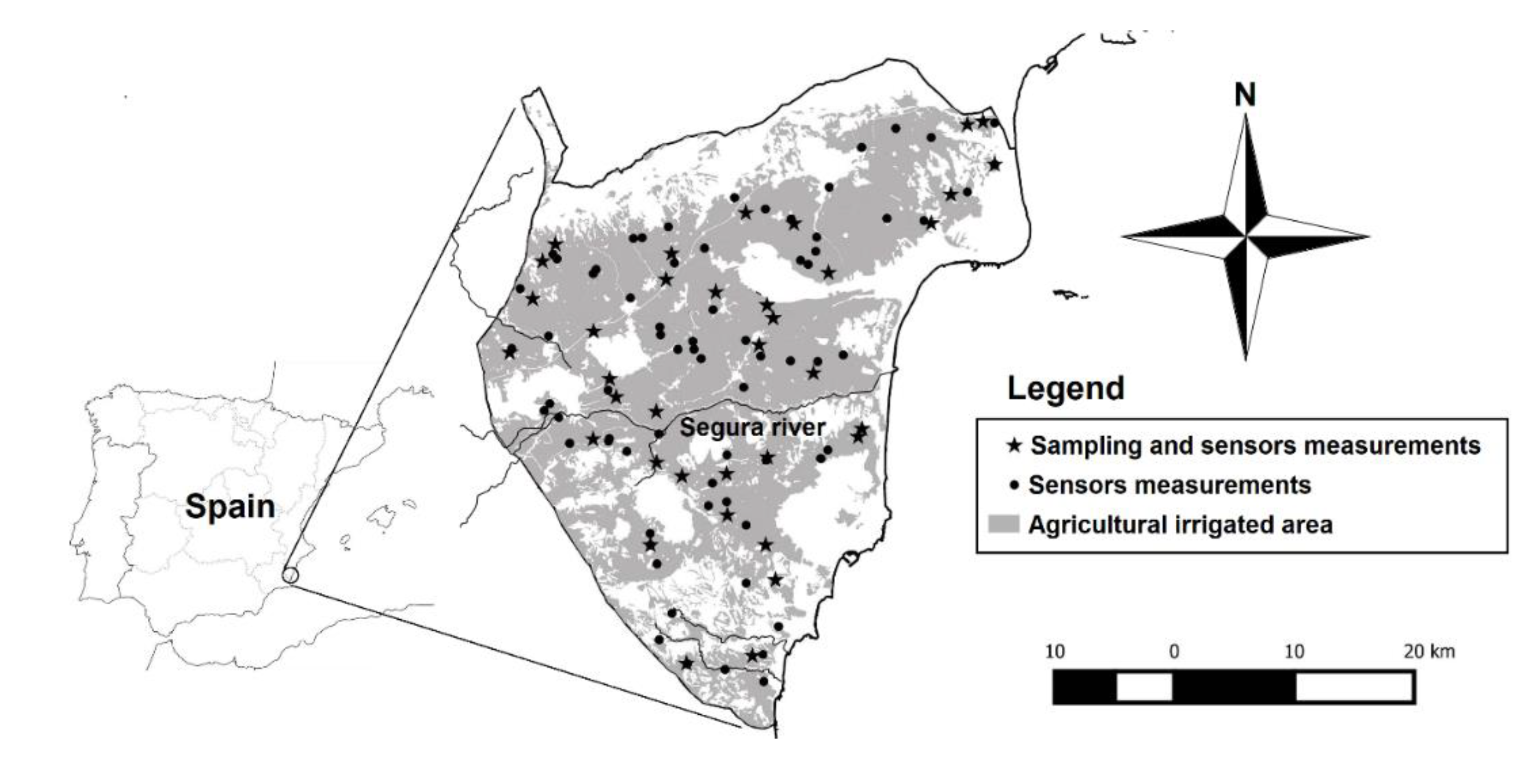
The Vega Baja del Segura and Baix Vinalopó jointly constitute an area in south-eastern Spain with over 55,000 ha under irrigation (Figure 1). This area is salt-threatened because of the low quality of the irrigation waters, the aridity of the climate, and the limitations for land drainage [45].

3.2. Survey Design

A systematic-random sampling design was applied to the entire study area and used to gather a dataset of measurements and sampling agricultural irrigated sites that were representative, thus capturing the soil variability but avoiding bias [46]. Specifically, a total of 107 sites were selected for the measurement of the soil electrical conductivity with the probes SCT-10, EM38, and WET-2 (Figure 1). From these, 37 sites were also sampled, as is described in the following subsection (Figure 1).

3.3. Soil Field Measurements and Sampling

In each site, first of all, the EM38 was set up away from the target spot by leaving the instrument to warm-up in the shade for 15 min, then by switching the I/P and Q/P controls to have a zero measurement with the instrument laying on a sufficiently large expanse of homogeneous low-conductive ground, e.g., the access road, and finally, by switching the Q/P control to have a measurement in the vertical dipole mode double than in the horizontal one at 1.5 m height.

Once the EM38 setup was finished, the EM38 was taken to the exact target agricultural site and the σ_b* measurements were taken in the vertical and horizontal dipole orientations at five different heights over the ground: 0, 50, 100, 150, and 200 cm.

Next, just below the center of the EM38, the WET-2 was used to take its corresponding σ_b, ε_b, and T measurements at the soil surface (0 cm) and additionally, by drilling with a Riverside auger, at 10, 30, and, either 50 or 60 cm depending on soil compactness. The extracted soil was separately collected from the 0–10, 10–30, 30–65, and 65–95 depth intervals, saved in plastic bags, and carried to the laboratory.

Additionally, on a spot 1 to 2 m from the center of the EM38, another hole was drilled with another narrower auger and the SCT-10 measurements of σ_b and T were taken at the following depths: 10, 30, 50, 60, 70, and 80 cm providing there was good enough contact between the probe electrodes and the soil.

3.4. Soil Laboratory Determinations

In the laboratory the soil samples were first of all analyzed for field water mass fraction (w_w) by weighing a representative subsample, oven-drying at 105 °C for 24 h, and weighing again. Then, the whole samples were spread out on trays, left to air-dry, and gently deaggregated to pass a 2-mm mesh sieve. The air-dried fine earths were then analyzed for hygroscopic water mass fraction (w_h), saturated paste water mass fraction (w_e), electrical conductivity at 25 °C in the saturation extract (σ_e), clay mass fraction (w_c), and soil organic matter mass fraction (w_om) using the ensuing methods.

The saturated soil pastes were prepared according to Rhoades [47], but using deionized water (σ₂₅ ≈ 1 μS/cm) as the only reagent in the entire procedure, allowing the soil-water mixtures to equilibrate for approximately four hours and taking a subsample for w_e determination, which was done by means of oven-drying at 105 °C for 24 h. Then, the saturation extract was obtained by suction with a vacuum system, and the σ_e was measured within one hour of extract collection with a microCM 2201 conductivity meter (Crison Instruments S.A., Barcelona, Spain) equipped with a conductivity cell of 1.1 cm⁻¹ constant.

The clay, along with the silt and sand mass fractions according to the USDA, were determined using the Bouyoucos densimeter method [48]. The soil organic matter mass fraction was determined following the Walkley-Black procedure [49].

3.5. Calculation of the σ_b Values for the Sampled Soil Layers

The σ_b and T values of the four soil layers in which the soil was split for sampling, i.e., 0–10, 10–30, 30–65, and 65–95, were calculated from the probe measurements at the point soil depths at which these latter were made, as is explained in the following. These soil-depth-standardized σ_b and T values were then used for all the comparisons and models.

3.5.1. From the Martek SCT-10 and Delta-T WET-2 σ_b Measurements

In the case of the SCT-10 and WET-2 probes, the σ_b and T values corresponding to the sampled soil depth intervals were calculated by linear interpolation, taking the mid depths of 5, 20, 47.5, and 80 cm for, respectively, the 0–10, 10–30, 30–65, and 65–95 cm depth layers.

3.5.2. From the Geonics EM38 σ_b* Measurements

In the case of the EM38, the σ_b of the aforementioned layers in addition to the soil below 95 cm were assessed from the σ_b* measurements in both dipole orientations and heights over the ground by the inverse matrix multiplication of Equation (6). However, since all the σ_b* measurements were highly correlated, this inverse problem was computationally ill-defined and could not be addressed the simply way.

A Tikhonov regularization in which the minimum of the following target function (Φ) is searched trying different values of the λ parameter has been found to satisfactorily sort out the aforementioned problem [41,42]:

$${\mathrm{\Phi }}_{\mathrm{A}}={\displaystyle \sum _{i=1}^{2m}{({\sigma }_{\mathrm{b}(\mathrm{X}{h}_i)}*-{\sigma }_{\mathrm{b}(\mathrm{X}{h}_i)}*\prime )}^2+{\lambda }^2{\displaystyle \sum _{j=1}^n{\displaystyle \sum _{k=1}^n{(l_{jk}{\sigma }_{\mathrm{b}(d_k)})}^2}}}$$

(14)

In Equation (14), X stands for V (vertical) or H (horizontal), σ_b(Xhi)* and σ_b(Xhi)*′ are, respectively, the observed and predicted depth-weighted electrical conductivity in the X dipole mode at the h_i height, and l_jk is the element of the jth row and kth column of the following second derivative matrix L (Equation (15)):

$$L=\left[\begin{array}{ccccc}-2& 1& 0& \dots & 0\\ 1& -2& 1& \dots & 0\\ 0& 1& -2& \dots & 0\\ \dots & \dots & \dots & \dots & 1\\ 0& 0& 0& 1& -2\end{array}\right]$$

(15)

In this work different values of the λ parameter within the range from 0 to 2 were used, and the value that featured the vertex of the L-shaped curve that arises when the first term on the right is graphed against the second one was selected as the most adequate for each site.

After the σ_b calculations were done, the hypothesis of low enough conductivity was checked through the calculation of the soil induction number N_B

N_B = s·(μ₀·ω·σ_{b_m}/2)^1/2

(16)

where σ_{b_m} is the depth-average soil conductivity calculated according to:

σ_{b_m} = (Σ σ_b(d_j)·Δd_j)/Σ Δd_j

(17)

where σ_b(d_j) and Δd_j are, respectively, the σ_b and thickness of the dj soil layer.

3.6. Calculation of σ_b at 25 °C (σ_b,25)

The SCT-10 calculates the bulk soil electrical conductivity at 25 °C (σ_b,25) and offers this value to the user, however, the EM38 and the WET-2 do not. For these latter two probes, the σ_b,25 was calculated from σ_b by applying the same equation used by the SCT-10 (Equation (2)) along with the temperature measured by the WET-2.

3.7. Data Analyses

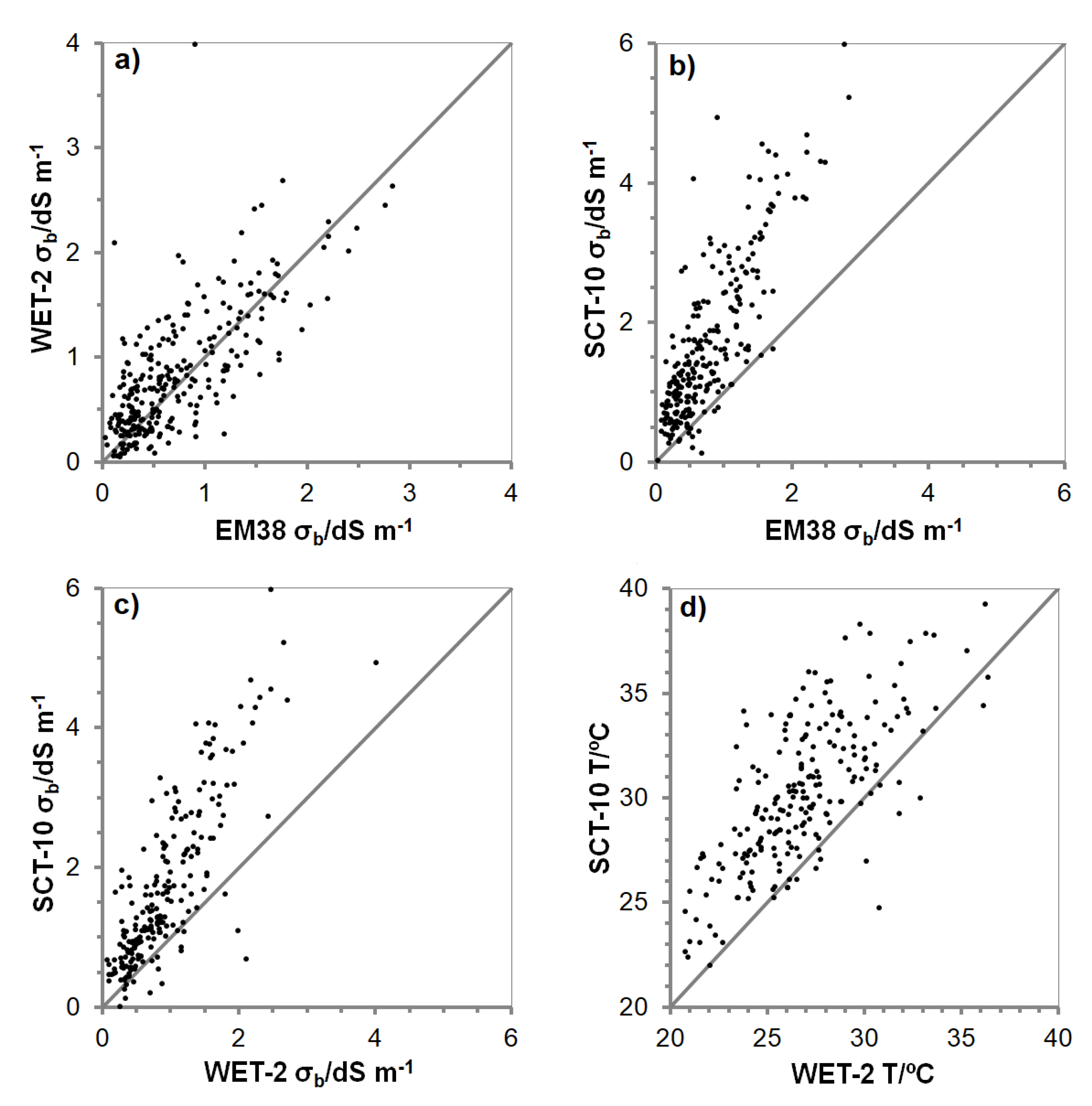
The values of σ_b obtained with each probe were pairwise compared, first graphically and then analytically, by testing the equality to zero of the mean standardized difference with the aid of the Student’s t-test [50].

Next, the three probes were further compared by developing multiple linear regression (MLR) models in order to assess the σ_e from the σ_b measurements, additionally finding out whether the inclusion of other soil properties, either measured, calculated, or determined in the laboratory may improve the model’s prediction ability. In order to know in which order these properties should be tried to be included in the corresponding MLR model, the Pearson’s product moment correlation coefficients of σ_e with each property were calculated in advance for the sites and depths for which the specific probe measurements were available. Then, the MLR models were built, including one property at a time from the highest to the lowest correlation coefficient in absolute value. Every time one new property was included in the model, the equality to zero of its regression coefficient was tested using the Student’s t-test. If the regression coefficient was different from zero at the 95% confidence level, the property was kept in the model, otherwise it was dropped. In this way, the ability of the probes to assess the σ_e was evaluated by means of the coefficients of determination, the root mean standard errors (RMSE), and the Lin’s concordance correlation coefficients [51] of the MLR models, as well as the significance of the regression coefficients. All the statistical analyses were carried out with the R software [52].

4. Results

4.1. Soil Determinations

The soils in the study area range in soil texture from silty clay to sandy loam with clay mass fractions from as low as 0.15 g g⁻¹ to as high as 0.69 g g⁻¹ with mean of 0.36 ± 0.02 g g⁻¹ with barely any differences among depths, while the soil organic matter mass fractions were found between 0.007 and 0.046 g g⁻¹ with mean of 0.021 ± 0.003 g g⁻¹ in the topsoil (

Table 2. Statistical summary of the data on saturation extract electrical conductivity at 25 °C (σ_e) and field water (w_w), clay (w_c), and organic matter (w_om) mass fractions in the different sampled depth intervals.

Depth Interval/cm	0–10	10–30	30–65	65–95
σe/dS m−1
Count	37	36	31	30
Mean	4.34	3.88	4.77	4.58
Std. Dev.	2.37	2.33	3.13	2.55
Maximum	11.24	10.84	13.76	13.50
Minimum	0.72	1.08	1.35	1.19
Skewness	4.679	3.758	5.566	3.260
ww/g g−1
Count	37	36	31	29
Mean	0.180	0.183	0.190	0.184
Std. Dev.	0.067	0.048	0.058	0.063
Maximum	0.320	0.270	0.374	0.378
Minimum	0.058	0.085	0.089	0.084
Skewness	3.012	−1.224	2.152	−0.417
wc/g g−1
Count	37	36	31	30
Mean	0.354	0.363	0.359	0.381
Std. Dev.	0.095	0.093	0.118	0.145
Maximum	0.592	0.622	0.613	0.691
Minimum	0.173	0.211	0.168	0.152
Skewness	0.700	3.664	3.663	0.657
wom/g g−1
Count	37	36	31	30
Mean	0.021	0.012	0.008	0.006
Std. Dev.	0.009	0.006	0.005	0.003
Maximum	0.046	0.025	0.021	0.012
Minimum	0.007	0.004	0.002	0.002
Skewness	4.430	3.261	2.390	2.424

). The σ_e was between 0.72 and 13.8 dS m⁻¹ with mean of 4.4 ± 0.4 dS m⁻¹, thus indicating that the area is salt-affected. The field water mass fraction was between 0.058 and 0.378 g g⁻¹ with mean of 0.18 ± 0.01 g g⁻¹. Regarding the probability distributions of the soil properties, the Pearson’s skewness coefficients were well over 1 for most of them, and thus they were positively skewed in general.

4.2. Probe Measurements

The σ_b measurements were between 0.03 and 6.00 dS m⁻¹ with mean of 1.70 ± 0.14 dS m⁻¹ for the SCT-10 probe with distributions heavily positively skewed (

Table 3. Statistical summary of the soil bulk electrical conductivity (σ_b) and temperature (T) measurements taken in the study area with the SCT-10 at different depths.

Depth/cm	10	30	50	60	70	80
σb/dS m−1
Count	82	92	84	69	25	11
Mean	1.33	1.74	2.05	2.28	1.61	2.17
Std. Dev.	0.95	1.11	1.31	1.41	1.32	2.09
Maximum	4.98	4.83	5.97	6.05	6.40	7.59
Minimum	0.03	0.21	0.15	0.27	0.16	0.60
Skewness	6.856	8.301	8.721	10.747	3.632	3.841
T/°C
Count	82	92	84	69	25	11
Mean	31.6	29.7	28.8	28.0	27.2	26.5
Std. Dev.	3.7	3.3	3.0	2.9	2.6	2.0
Maximum	39.4	37.6	36.1	35.3	32.6	28.7
Minimum	22.4	22.6	22.1	21.8	22.4	22.6
Skewness	2.305	1.732	5.066	3.494	0.579	1.633

), and between 0.06 and 4.00 dS m⁻¹ with mean of 0.86 ± 0.07 dS m⁻¹ for the WET-2 with distribution also very positively skewed (

Table 4. Statistical summary of the soil bulk electrical conductivity (σ_b), relative dielectric permittivity (ε_b), and temperature (T) measurements taken in the study area with the WET-2 at different depths.

Depth/cm	0	10	30	50
σb/dS m−1
Count	103	104	99	67
Mean	0.67	0.80	0.96	1.13
Std. Dev.	0.62	0.49	0.61	0.70
Maximum	4.19	2.87	2.87	2.83
Minimum	0.04	0.09	0.14	0.13
Skewness	9.311	4.388	6.928	6.756
εb
Count	103	104	99	67
Mean	23.90	26.59	27.76	27.60
Std. Dev.	9.34	7.66	8.68	8.66
Maximum	55.59	42.81	46.94	45.14
Minimum	8.11	9.61	12.69	11.73
Skewness	3.349	0.651	−0.744	0.590
T/°C
Count	103	104	99	67
Mean	28.91	26.57	25.80	25.18
Std. Dev.	3.76	2.59	2.29	2.44
Maximum	38.00	32.60	32.20	30.30
Minimum	20.80	20.70	20.60	20.70
Skewness	3.326	0.817	−2.578	−0.180

). The σ_b* measured with the EM38 on the soil surface were between 0.03 and 2.47 dS m⁻¹ in the vertical dipole mode and between 0.05 and 2.21 dS m⁻¹ in the horizontal one with data very positively skewed (

Table 5. Statistical summary of the soil depth-weighted electrical conductivity measurements taken in the study area with the EM38 in the vertical (σ_bV*) and horizontal (σ_bH*) dipole modes at different heights.

Height/cm	0	50	100	150	200
σbV*/dS m−1
Count	107	107	107	107	107
Mean	0.79	0.44	0.30	0.22	0.16
Std. Dev.	0.55	0.29	0.19	0.14	0.09
Maximum	2.47	1.31	0.90	0.57	0.40
Minimum	0.03	0.01	0.01	0.00	0.00
Skewness	7.555	8.965	8.093	7.045	5.457
σbH*/dS m−1
Count	107	107	107	107	107
Mean	0.70	0.22	0.15	0.10	0.08
Std. Dev.	0.44	0.14	0.09	0.07	0.05
Maximum	2.21	0.62	0.41	0.28	0.20
Minimum	0.05	0.00	−0.03	−0.04	−0.05
Skewness	9.148	6.785	8.664	6.546	5.000

). The σ_b* values systematically decreased as the instrument was lifted (Table 5). The σ_b data obtained from the EM38 σ_b* measurements by the inversion of Equation (6) were between 0.02 and 2.83 dS m⁻¹ with mean of 0.71 ± 0.04 dS m⁻¹ (

Table 6. Statistical summary of the soil bulk electrical conductivity at different soil depth intervals estimated by inversion of Equation (6) in the soils of the study area using the Tikhonov regularization and the induction numbers (N_B) calculated using Equation (16).

Depth Interval/cm	0–10	10–30	30–65	65–95	>95	NB
σb/dS m−1
Count	107	107	107	107	107	107
Mean	0.43	0.78	0.95	0.87	0.54	0.055
Std. Dev.	0.27	0.50	0.62	0.57	0.36	0.019
Maximum	1.36	2.40	2.83	2.57	1.61	0.101
Minimum	0.02	0.04	0.04	0.04	0.02	0.012
Skewness	8.445	9.031	9.367	9.166	8.349	4.280

), and the corresponding induction numbers were between 0.012 and 0.101 with mean of 0.055 ± 0.004 (Table 6), which can be considered remarkably lower than the unity (N_B << 1). This gives support to the hypothesis of low-to-moderate conductivity of the soils of the study area and therefore, to the use of the linear model represented by Equation (6) for σ_b calculation. All the σ_b data calculated from the EM38 measurements presented very positively-skewed distributions in resemblance to the SCT-10 and WET-2 σ_b values.

Regarding the rest of the probe measurements, the temperature registered with the SCT-10 was between 21.0 and 39.3 °C with mean of 30.0 ± 0.4 °C, while the WET-2 measured temperatures were between 20.7 and 37.2 with mean of 26.9 ± 0.4 °C. The soil relative bulk dielectric permittivity was only measured with the WET-2 and was between 9.0 and 53.6 with mean of 26 ± 1.

4.3. Comparison of σ_b Values

The EM38 σ_b calculated data was, with r = 0.73, remarkably correlated with the WET-2 σ_b measurements (Figure 2a). Besides, in spite of the wide range of differences between the EM38 and the WET-2 measurements, which was 4.0 dS/m, the mean difference was only −0.13 dS/m. However, according to the test of the normalized difference, this value, though small, was significantly different from zero (p < 0.001), which indicates that the EM38 gave, on average, slightly lower σ_b values than the WET-2.

Regarding the SCT-10, even though its σ_b measurement exhibited even higher correlation with either the EM38 or the WET-2 σ_b, i.e., respectively, r = 0.83 and r = 0.82, it was on average much higher than whichever of them, specifically, 0.94 dS/m higher than the EM38 σ_b and 0.81 dS/m higher than the WET-2 σ_b (Figure 2b,c). This disagreement was observed even in the temperature, with the SCT-10 consistently measuring higher than the WET-2, specifically, 3.4 °C more on average (Figure 2d).

4.4. Development of Models for σ_e Estimation

4.4.1. The Martek SCT-10

With a correlation coefficient of 0.55 the property correlated the most with the σ_e was the σ_b. This was followed by temperature, the organic matter, the clay, and the field water mass fractions (

Table 7. Pearson’s product-moment correlation coefficients among the SCT-10 probe measurements and calculations and soil properties in the sites and depths the former were available.

	σb	T	σb,25	σe	ww	wc
T	0.053
σb,25	0.994	−0.022
σe	0.548	0.144	0.521
ww	0.564	−0.172	0.567	0.041
wc	0.320	0.197	0.307	−0.054	0.310
wom	−0.004	0.345	−0.040	0.132	0.092	0.312

). Interestingly, the correlation of σ_e dropped to 0.52 when the temperature-standardized σ_b,25 was used instead of σ_b.

According to the order of the correlation coefficients, the properties σ_b, T, w_om, w_c, and w_w were tried to be included following this succession in an increasingly complex MLR for σ_e estimation with the SCT-10 probe. The simple linear regression model using σ_b explained 30% of variance (

Table 8. Coefficients of determination and regression along with their standard errors, student’s t and p values for the different multiple linear regression models developed to estimate the saturation extract electrical conductivity at 25 °C (σ_e), where the best most parsimonious model for each probe has been highlighted in italics.

Model Number	Probe	R2	Regress. Coeff.	σb	εb1/2	T	ww	wc	wom
1	SCT-10	0.300	Value	1.19	‒	‒	‒	‒	‒
			Std. Dev.	0.20	‒	‒	‒	‒	‒
			t	5.96	‒	‒	‒	‒	‒
			p	<0.001	‒	‒	‒	‒	‒
2	SCT-10	0.326	Value	1.20	‒	0.12	‒	‒	‒
			Std. Dev.	0.20	‒	0.06	‒	‒	‒
			t	6.10	‒	1.79	‒	‒	‒
			p	<0.001	‒	0.078	‒	‒	‒
3	SCT-10	0.318	Value	1.19	‒	‒	‒	‒	40.95
			Std. Dev.	0.20	‒	‒	‒	‒	27.88
			t	6.01	‒	‒	‒	‒	1.47
			p	<0.001	‒	‒	‒	‒	0.146
4	SCT-10	0.359	Value	1.37	‒	‒	‒	−6.00	‒
			Std. Dev.	0.20	‒	‒	‒	2.20	‒
			t	6.74	‒	‒	‒	−2.73	‒
			p	<0.001	‒	‒	‒	0.008	‒
5	SCT-10	0.441	Value	1.77	‒	‒	−15.10	−4.80	‒
			Std. Dev.	0.22	‒	‒	4.36	2.09	‒
			t	7.94	‒	‒	−3.46	−2.30	‒
			p	<0.001	‒	‒	<0.001	0.024	‒
6	EM38	0.203	Value	2.00	‒	‒	‒	‒	‒
			Std. Dev.	0.34	‒	‒	‒	‒	‒
			t	5.81	‒	‒	‒	‒	‒
			p	<0.001	‒	‒	‒	‒	‒
7	EM38	0.203	Value	2.00	‒	‒	0.00006	‒	‒
			Std. Dev.	0.35	‒	‒	0.02386	‒	‒
			t	5.67	‒	‒	0.00272	‒	‒
			p	<0.001	‒	‒	0.998	‒	‒
8	EM38	0.310	Value	2.97	‒	‒	‒	−9.10	‒
			Std. Dev.	0.39	‒	‒	‒	2.02	‒
			t	7.67	‒	‒	‒	-4.50	‒
			p	<0.001	‒	‒	‒	<0.001	‒
9	EM38	0.336	Value	3.20	‒	‒	‒	−10.58	54.36
			Std. Dev.	0.39	‒	‒	‒	2.10	23.84
			t	8.11	‒	‒	‒	−5.05	2.28
			p	<0.001	‒	‒	‒	<0.001	0.024
10	WET-2	0.303	Value	2.46	‒	‒	‒	‒	‒
			Std. Dev.	0.39	‒	‒	‒	‒	‒
			t	6.22	‒	‒	‒	‒	‒
			p	<0.001	‒	‒	‒	‒	‒
11	WET-2	0.518	Value	5.53	−2.56	‒	‒	‒	‒
			Std. Dev.	0.59	0.41	‒	‒	‒	‒
			t	9.34	−6.26	‒	‒	‒	‒
			p	<0.001	<0.001	‒	‒	‒	‒
12	WET-2	0.594	Value	5.71	−2.51	0.23	‒	‒	‒
			Std. Dev.	0.55	0.38	0.06	‒	‒	‒
			t	10.41	−6.63	4.04	‒	‒	‒
			p	<0.001	<0.001	<0.001	‒	‒	‒
13	WET-2	0.608	Value	5.61	−2.30	0.23	‒	−3.34	‒
			Std. Dev.	0.55	0.39	0.06	‒	1.93	‒
			t	10.29	−5.85	4.15	‒	−1.73	‒
			p	<0.001	<0.001	<0.001	‒	0.087	‒
14	WET-2	0.594	Value	5.73	−2.51	0.22	‒	‒	5.42
			Std. Dev.	0.56	0.38	0.06	‒	‒	23.34
			t	10.29	−6.59	3.69	‒	‒	0.23
			p	<0.001	<0.001	<0.001	‒	‒	0.817

, model number 1). The inclusion of either the temperature or the organic matter content barely increased R². The regression coefficients of both were not either different from zero at the 95% confidence level and therefore, they were eventually not included in the model for σ_e estimation (Table 8, model numbers 2 and 3). On the contrary the inclusion of the clay mass fraction and the field water mass fraction did increase R² and moreover, their regression coefficients were different from zero at the 95% level, thus being eventually kept in a model of the form: σ_e = a σ_b + b w_c + c w_w (Table 8, model numbers 4 and 5). This last model explained 44% of the variance in the σ_e data and had RMSE of 1.8 dS m⁻¹ (44%). The fit between predictions and measurements of σ_e according to model 5 can be appreciated in Figure 3a, with an associated Lin’s concordance correlation coefficient equal to 0.61.

4.4.2. The Geonics EM38

With a correlation coefficient of 0.45 the property correlated the most with the σ_e was the σ_b. This was followed by the field water, the clay and the organic matter mass fractions (

Table 9. Pearson’s product-moment correlation coefficients among the EM38 σ_b calculated values, and soil properties in the sites and depths the former were available.

	σb	σb,25	σe	ww	wc
σb,25	0.996
σe	0.451	0.434
ww	0.466	0.408	0.092
wc	0.559	0.477	−0.019	0.435
wom	−0.088	−0.098	0.014	0.133	0.206

). Similarly to what happened with the SCT-10, the correlation with σ_e dropped to 0.43 when the temperature-standardized σ_b,25 was used instead of σ_b.

In accordance with the calculated correlation coefficients, the properties σ_b, w_w, w_c, and w_om were tried to be included in this order in an increasingly complex MLR for σ_e estimation with the EM38 instrument. The simple linear regression model using σ_b explained 20% of variance (Table 8, model number 6). The inclusion of the field water mass fraction did not increase R². This fact, along with a regression coefficient not different from zero at the 95% confidence level, made this property not be included in the eventual model for σ_e estimation (Table 8, model number 7). Contrary to this, the inclusion of the clay and the organic matter mass fractions did increase R² and moreover, since their regression coefficients were different from zero at the 95% level, both were kept in a model of the form: σ_e = a σ_b + b w_c + c w_om (Table 8, model numbers 8 and 9). This last model explained 34% of variance and had RMSE of 2.1 dS m⁻¹ (48%). The fit between predictions and measurements of σ_e according to model 9 can be appreciated in Figure 3b, which presents a Lin’s concordance correlation coefficient equal to 0.50.

4.4.3. The Delta-T WET-2

With a correlation coefficient of 0.55, the property correlated the most with the σ_e was again the σ_b, this was followed by the ε_b^1/2, the temperature, the clay, and the organic matter mass fractions (

Table 10. Pearson’s product-moment correlation coefficients among the WET-2 probe measurements and calculations and soil properties in the sites and depths the former were available.

	σb	T	σb,25	εb	σp	εb1/2	σe	ww	wc
T	−0.166
σb,25	0.995	−0.241
εb	0.838	−0.194	0.836
σp	0.904	−0.222	0.907	0.607
εb1/2	0.821	−0.207	0.820	0.995	0.610
σe	0.551	0.180	0.525	0.187	0.705	0.199
ww	0.641	−0.216	0.639	0.822	0.419	0.825	0.078
wc	0.263	−0.029	0.269	0.379	0.130	0.383	−0.091	0.379
wom	−0.181	0.363	−0.209	−0.113	−0.283	−0.113	−0.023	0.139	0.266

). Interestingly again, the correlation with σ_e dropped to 0.53 when the temperature-standardized σ_b,25 was used instead of σ_b.

On the basis of the order found for the correlation coefficients, the properties σ_b, ε_b^1/2, T, w_c, and w_om were tried to be included following this sequence in an increasingly complex MLR model for σ_e estimation with the WET-2 probe. The simple linear regression model using σ_b was able to explain 30% of variance (Table 8, model number 10). The inclusion of ε_b^1/2, which was calculated from the WET-2 ε_b measurement, remarkably increased R². This fact alongside a regression coefficient very significantly different from zero (p < 0.001) made this property be kept in the eventual model for σ_e estimation (Table 8, model number 11). The inclusion of the WET-2-measured temperature appreciably increased R² again. Since the temperature had also a regression coefficient very significantly different from zero (p < 0.001), it was also kept in the model (Table 8, model number 12). Contrary to this, the inclusion of the mass fractions of either the clay or the organic matter did not noticeably increase R² and moreover, their regression coefficients were not different from zero at the 95% confidence level (Table 8, model numbers 13 and 14). As a consequence, these last two laboratory-determined properties were not included in the eventual model for σ_e estimation, and an equation of the form σ_e = a σ_b + b ε_b^1/2 + c T could be accepted for the WET-2 probe. This model explained 59% of variance and had RMSE of 1.7 dS m⁻¹ (38%). The fit between predictions and measurements of σ_e according to the best most parsimonious model for the WET-2 σ_b, ε_b^1/2 and T data can be appreciated in Figure 3c, which features a Lin’s concordance correlation coefficient equal to 0.74.

In accordance with the correlation coefficients calculated between σ_e and the probe measurements and calculations, the σ_p given by Equation (12) was remarkably more correlated with σ_e (r = 0.71) than whichever of the σ_b measurements (0.45 ≤ r ≤ 0.55). Therefore, whether the use of σ_p instead of σ_b would improve the MLR model obtained for the WET-2 was tested with the replacement of σ_b by σ_p in model 12 (Table 8). The model with the form σ_e = a σ_p + b ε_b^1/2 + c T preserved all the regression coefficients significantly different from zero (p < 0.001), and was able to explain 69% of the variance in the σ_e data with a RMSE of 1.5 dS m⁻¹ (33%). The fit between predictions and measurements of σ_e according to this model for the WET-2 σ_p, ε_b^1/2 and T data can be appreciated in Figure 3d, which presents a Lin’s concordance correlation coefficient equal to 0.81.

5. Discussion

Nowadays, soil scientists and practitioners have different techniques available for salinity appraisal by means of σ_b measurements. These techniques can be arranged in order of increasing complexity and hence age, from first to last: Electrical resistance (ER), electromagnetic induction (EMI), time domain reflectometry (TDR), and frequency domain reflectometry (FDR). In this work, three out of these four were compared, namely, ER, EMI, and FDR, by means of classical devices, respectively, the Martek SCT-10, the Geonics EM38, and the Delta-T WET-2. The σ_b measurements taken with all three instruments were moderate-to-highly correlated, however, not only scattering occurred, but also remarkable systematic deviations. These happened mainly between the SCT-10 probe and the other two because this ER sensor gave consistently higher σ_b measurements.

In the case of the EM38, which is a contactless technique, the σ_b values were not measured but, alternatively, they had to be calculated by means of the inversion of Equation (6). This 1D inversion uses the sensitivity functions developed by McNeill [40], which were derived from an asymptotic approximation to the Maxwell’s equations and are valid as long as the ability of the soil to attenuate the primary magnetic field of the EMI instrument is not too high. This occurs when the soils are not very conductive or, in other words, when the induction number is low enough (N_B << 1). According to different researches, the limit between low and high induction numbers (N_B) lays somewhere between 0.32 and 0.02 [53]. In our work, they have been estimated to be between 0.012 and 0.101 with mean of 0.055, i.e., closer to the lower part of that range than to the higher one, thus giving us confidence that the low induction number hypothesis was acceptably fulfilled.

Therefore, assuming that the McNeill’s approach to Maxwell’s equations is acceptable for most of our soils, the σ_b values calculated by inversion of Equation (6) using Equations (4) and (5) are considered to adequately correspond to true σ_b values [53], i.e., those that would be measured by a reliable direct contact technique, e.g., either ER, FDR, or TDR. In our case, the dispersion between the EM38-calculated σ_b values and the WET-2 σ_b measurements can be attributed in an important extent to the very different soil volumes sensed by each probe as shown in Table 1, which was also a cause indicated by Coppola et al. [18] when comparing between EMI and TDR. However, in spite of this fact, on average, the EM38-calculated σ_b data were very similar to the WET-2 measurements thus boosting our confidence that the 1D inversion of Equation (6) had been appropriate.

The systematic departures in the SCT-10 measurements in comparison to the other two devices were even observed in the temperature. However, in spite of these differences all three instruments may still be profitably used for soil salinity appraisal provided probe-specific and maybe site-specific calibrations are developed. In this regard, modelling for σ_e estimation on the basis of only σ_b led to very poor models, mainly with the EM38 (R² = 0.20), but also with the SCT-10 and the WET-2 probes (R² = 0.30 both). Interestingly, the use of temperature-standardized measurements worsened the models. This fact indicates that an equation like Equation (2), which has been developed for aqueous solutions, does not satisfactorily work for the bulk soils. This is an already observed effect, which has been explained on the basis of the contribution to σ_b from the exchange ions within the bound soil water, whose conductivity would increase with temperature more steeply than the conductivity of the ions within the free soil water [54]. Therefore, since the soils of the study area are remarkably clayey, temperature should be included in the models for σ_e estimation, however, this must not be done with equations developed for aqueous systems, but through an alternative means. The inclusion of the temperature as another factor within an empirical MLR model was tried as this alternative in this research and it worked better, although significantly only for the WET-2 probe (p < 0.05).

Besides, since the σ_b is known to depend not only on salinity and temperature, but on several soil properties [9,10,11,12,14], other ground attributes were checked in the MLR models for σ_e estimation as has been done by other researchers [55]. These properties were selected considering the most influential on the σ_b* measurements taken with the EM38 (unpublished results): w_c, θ_w, bulk density (ρ_b), w_om, and T. Specifically, three of these properties were tried to be included as such since they had been either determined or measured (w_c, w_om and T), whereas for ρ_b no data was available, and for θ_w the inclusion was tried by means of surrogates, which were ε_b^1/2 in the case of the WET-2, and w_w, in the case of the SCT-10 and the EM38.

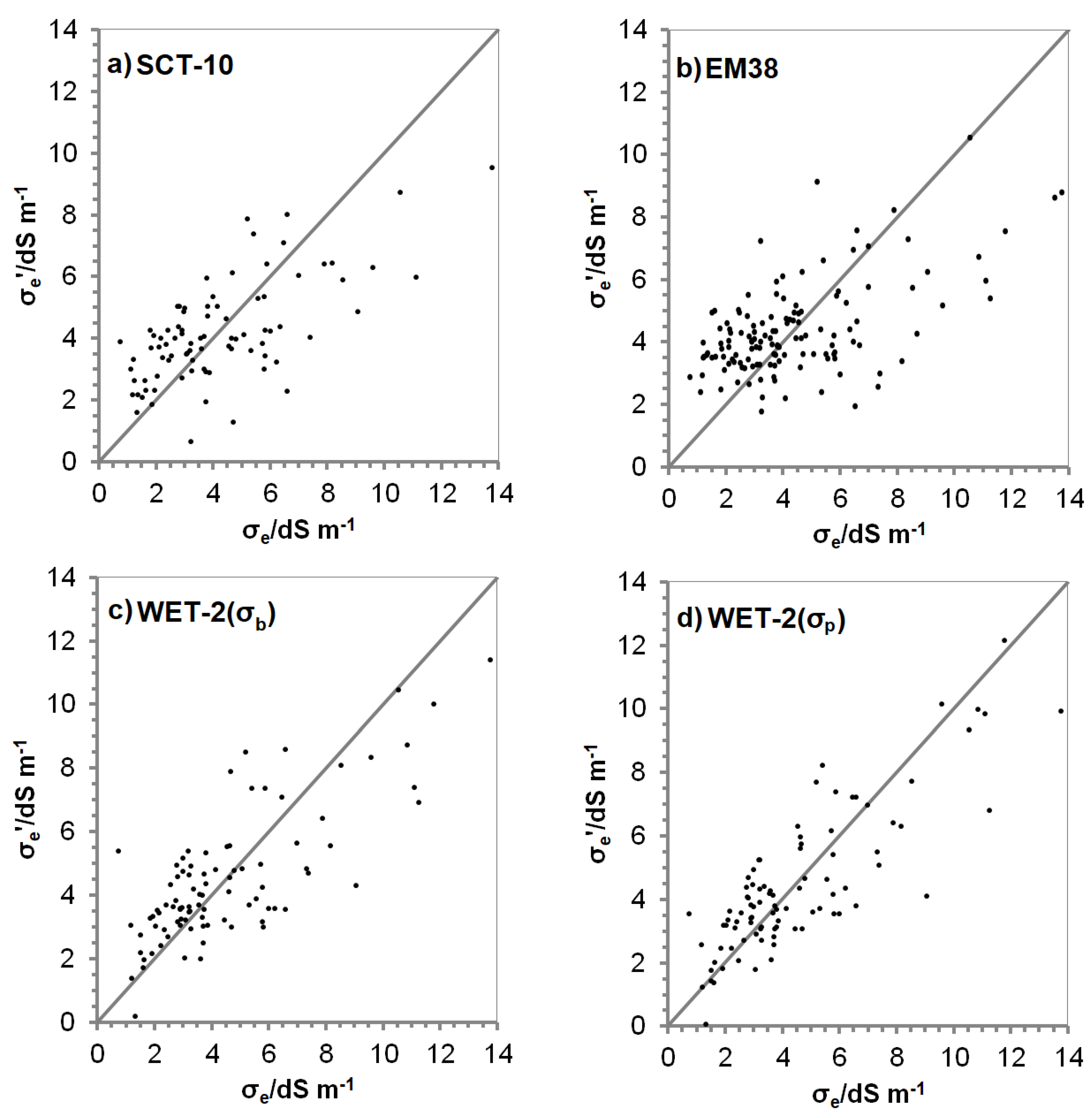
Certainly, the inclusion of other soil properties for the estimation of the σ_e and thus salinity appraisal improved the prediction, giving rise to models with R² and RMSE values of 0.44 and 1.8 dS m⁻¹, 0.34 and 2.1 dS m⁻¹, and 0.59 and 1.7 dS m⁻¹ for, respectively, the SCT-10, the EM38, and the WET-2. Apparently, these model performance coefficients do not compare well with the ones obtained in other works, e.g., Zemni et al. [34] achieved RMSE values below 1 dS m⁻¹ for a CCC probe, and Samson et al. [22] R² up to 0.98 for CCC and TDR probes. However, compared to theirs and other researchers’, the testing conditions of the study area in this work were very challenging because of its large extension and thus diversity of soils. This fact contrasts with the conditions of the aforementioned studies in which only one sandy soil was tested. Besides, in this work, the estimation of σ_e was tried, whereas in the aforesaid and most others’ the easier σ_p is tried. In any case, in this work, the use of θ_w instead of w_w and the additional use of ρ_b would have improved the models. Besides, the use of soil samples more representative of the actual soil volume sensed by the EM38 would have decreased the scattering of predicted against observed σ_e and hence increased R² and decreased RMSE. Finally, the use of different model approaches would have maybe improved a bit more the models’ prediction ability. Nevertheless, the development of the best possible model for each probe was not the objective of this investigation, but a means to compare among them.

Therefore, what it is interesting is to note that, whatever the case, in order to attain better estimation performances, the soil must be drilled regardless of the instrument that is used, even with the contactless EM38. Additionally, samples should be separately taken from different soil depth intervals and analyzed in the laboratory for field water and clay mass fractions in the case of the SCT-10, and for clay and organic matter mass fractions in the case of the EM38, but not in the case of the WET-2. This way of working overshadows some of the benefits of using sensors in the case of the SCT-10 and even more the EM38. On the contrary, in the case of the WET-2, only probe measurements were needed to develop an MLR model for σ_e estimation and therefore for salinity appraisal on the basis of σ_b. The use of the sensor-calculated σ_p instead of the sensor-measured σ_b further improved the σ_e estimation reaching a R² of 0.69. However, the RMSE was still 1.5 dS m⁻¹, which is somewhat far from satisfactory since the amplitude interval of the lower classes of salt affected soils is 2 dS m⁻¹ (

Table 11. Soil salinity assessment scheme for agriculture based on the threshold-slope model of crop yield decline. Re-elaborated from Richards et al. [58] and Ayers and Westcot [59].

†σet/dS m−1	Salt Affected Crops	†σea/dS m−1	Soil Salinity Class
<1.3	Sensitive	<2	Non saline
[1.3, 3)	Moderately sensitive	[2, 4)	Slightly saline
[3, 6)	Moderately tolerant	[4, 8)	Moderately saline
[6, 10)	Tolerant	[8, 16)	Strongly saline
≥10	Halophytes	≥16	Extremely saline

^†σ_et: Soil saturation extract electrical conductivity at 25 °C, over which yield starts to decline; σ_ea; Soil saturation extract electrical conductivity at 25 °C, over which yield drops below 90% of maximum for all classes except for the last one, for which it drops below 70% of maximum.

).

Given that working at higher frequencies is known to attenuate the effects of soil type, σ_b and T on the ε_b measurement [56], the use of frequencies over 20 MHz in WET-2-like FDR and TDR sensors such as the CS655 (Campbell Scientific, Inc., Logan, UT, USA), which uses two frequencies of 175 MHz and 100 MHz in order to better characterize σ_b and thus refine the ε_b measurement [57], is expected to enhance the soil salinity appraisal with the aim of diminishing the RMSE down to more acceptable values while keep using only sensor data.

6. Conclusions

The field comparison made between three classical commercial devices capable of EC detection, each one featuring a different physical foundation, i.e., ER, EMI, and FDR, revealed several interesting things related to the evolution the technology for field soil salinity appraisal has witnessed in the past forty years. The comparison has shown, first of all, that the use of one specific device determines the way of working not only because of the physical foundation of the σ_b measurement, but also because of the add-ons the specific devices include. These extra features can be additional measurements such as temperature, which is naturally and easily integrated with the aid of a built-in thermistor alongside contact techniques like ER (SCT-10) and FDR (WET-2), and relative dielectric permittivity, which can only be implemented in FDR and TDR technologies or integrated with the aid of the two-electrode ER technique in combined probes such as the modern capacitance-conductance (CCC) ones. These extra features can also be additional calculations such as the temperature-standardized σ_b,25, as well as θ_w and σ_p in FDR and TDR or CCC. Regarding temperature, it has been also shown that the evolution of temperature in aqueous solutions does not represent the evolution in bulk soils and that an alternative should be chosen, e.g., another factor in the framework of an MLR model. Finally, in this work it has been shown that an FDR contact probe like the WET-2 not only provided the best estimation model making use of the additional σ_p calculation, but also provided a balance between labor and information obtained because, even though with this contact device soil drilling is necessary to access the subsoil layers, it is also the only one in which soil sampling and laboratory analysis are not needed at all to develop a σ_e estimation model. The ongoing development of light weight non expensive FDR and TDR probes, specifically working at higher frequencies for enhanced ε_b and σ_b estimations, offers a promising way in which salinity appraisal is going to improve and made available for a greater audience. In the future, similar comparisons will be made, including the most recent commercial TDR and CCC probes.