Digital, Three-Dimensional Visualization of Root Systems in Peat

Abstract

Belowground plant structures are inherently difficult to observe in the field. Sedge peat that mainly consists of partly decayed roots and rhizomes offers a particularly challenging soil matrix to study (live) plant roots. To obtain information on belowground plant morphology, research commonly relies on rhizotrons, excavations, or computerized tomography scans (CT). However, all of these methods have certain limitations. For example, CT scans of peat cores cannot sharply distinguish between plant material and water, and rhizotrons do not provide a 3D structure of the root system. Here, we developed a low-cost approach for 3D visualization of the root system in peat monoliths. Two large diameter (20 cm) peat cores were extracted, frozen and two smaller peat monoliths (47 × 6.5 × 13 cm) were taken from each core. Slices of 0.5 mm or 1 mm were cut from one of the frozen monoliths, respectively, using a paper block cutter and the freshly cut surface of the monolith was photographed after each cut. A 3D model of the fresh (live) roots and rhizomes was reconstructed from the resulting images of the thinner slices based on computerized image analysis, including preprocessing, filtering, segmentation and 3D visualization using the open-source software Fiji, Drishti, and Ilastik. Digital volume measurements on the models produced similar data as manual washing out of roots from the adjacent peat monoliths. The constructed 3D models provide valuable insight into the three-dimensional structure of the root system in the peat matrix.

1. Introduction

About 20% of the global soil carbon is stored in peatlands [1]. Next to mosses, plant roots are an important constituent of global peats. In the temperate parts of Europe in particular, sedge dominated fens were once a dominant landscape feature [2]. Soil carbon sequestration in sedge peat is mainly through plant roots that are growing into deeper strata. After they die, the roots form new peat that displaces the existing peat matrix. Sedge peats are “displacement peat” [3,4], in which peat accumulates (“grows up”) through the addition of material belowground. An understanding of peat formation through displacement by roots starts with an understanding of root growth.

Although roots are of major importance for the individual plant, competitive interactions, and ecosystem processes, relatively little is known about them, because belowground structures of the vegetation are inherently difficult to study [5,6]. Thus, the development of new techniques for studying root systems is important to increase our understanding of the root system under field conditions. In situ examination of belowground plant biomass is often still limited to hand-sieving methods or mechanical root washers, which are time-consuming and error-prone methods [7] that do not provide information about the structure of the root system in the soil. The use of rhizotrons or minirhizotrons has been widely adopted to study root growth and demography in situ [8,9], but the method lacks accuracy in determining the actual spatial patterns of root systems, as it only produces 2D image data. In addition, only few attempts have been made to determine the in situ shape of root systems of vascular plants in peat soils [7,10,11,12], as these are even more challenging than mineral soils. Computed tomography (CT) can provide 3D images, and has been implemented successfully for roots in the soil matrix, however, this method is not suitable for peat soils. For example, 3D representations of Sphagnum peat structure using CT exist [13,14,15], but so far could only be applied on relatively small volumes of a few cubic centimeters. Moreover, these CT scans cannot sharply distinguish between (dead) plant material and water [13] and even in dried peat no sharp distinction can be made between live and dead roots. Davey et al. [7] used CT to examine the distribution of live coarse roots and rhizomes in peat marsh soils, but no 3D visualization could be derived from the image data. Thus, a low-cost method allowing for an in situ 3D visualization of belowground plant biomass that covers large peat soil volumes over several decimeters of depth, is hitherto not available.

Here, we present a serial section (tomography) workflow combined with (semi-)automated image analysis and 3D visualization techniques to create 3D models of in situ belowground plant biomass from peat monoliths. We use the model to determine the volume of different root fractions over depth and compare the findings with results from conventional sieving and washing of roots.

2. Materials and Methods

2.1. Sampling

Visualization methods were developed and tested on peat monoliths taken in September 2018 in the Relzower Wiesen in the Peene valley near Anklam, Mecklenburg-Western Pomerania, Germany. The sampling site was located ca. 170 m east of the B109 highway, south of the village of Relzow (N 53.879019, E 13.694643) at an altitude of 0 m above sea level (Supplementary Material Map S1). The Relzower Wiesen are a slightly degraded, but wet percolation mire consisting of sedge peat. Vegetation is dominated by Carex acutiformis, Molinia caerulea, Carex disticha, and Carex flacca. Phragmites australis grows in the immediate vicinity of the sampling site at a distance of two meters. The area is mown annually to suppress the expansion of Phragmites, most recently in the year before sampling.

Two cylindrical peat cores (diameter 20 cm) were extracted by means of a Clymo-corer [16]. The northern core with a length of 44.5 cm is referred to as “RWSN”, the southern core with a length of 42 cm as “RWSS”. Cores were transported upright and stored at −18 °C until further preparation.

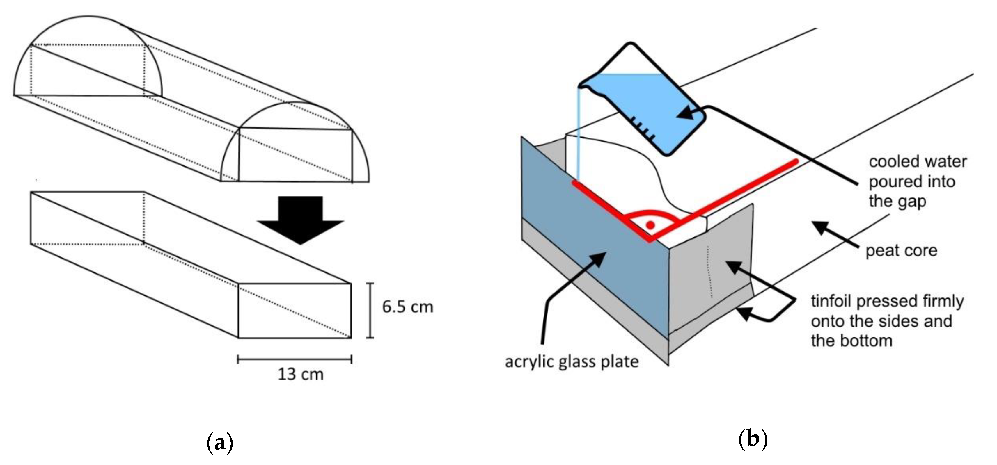
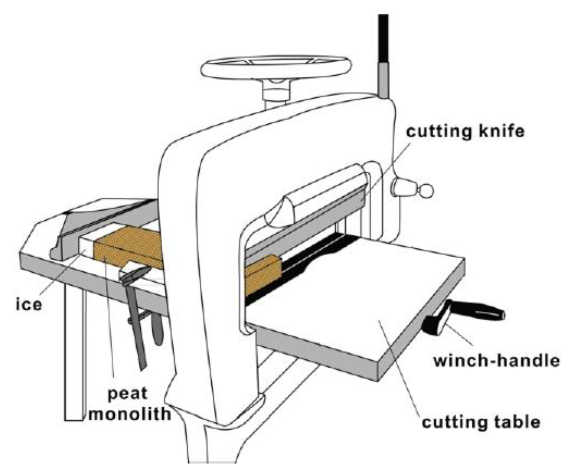
2.2. Sample Preparation

The frozen cores were cut longitudinally using an angle grinder for the PVC tubes and a coarse toothed pruning saw to cut the peat. One half of each core was prepared for sectioning with DAMOCLES [17], a device for cutting frozen peat, and the other half for root washing.

In order to be cut with DAMOCLES, the peat monoliths were cut with a pruning saw into bricks with a width of 13 cm and a height of 6.5 cm (Figure 1a). The surfaces of all sides were smoothed with a metal surform tool. An ice cap was added to the uneven surface of plants and litter at the top of the core to create a level surface perpendicular to the sides of the core. This cap increased the stability of the peat core along the guidance rod of DAMOCLES and moreover allowed sampling of the upper peat and litter strata. The best results in creating an ice cap were obtained using a mold made of acrylic glass and tinfoil joined together by hot glue (Figure 1b).

Sectioning with DAMOCLES (Figure 2) was done at a temperature of −5 °C in a freezing chamber. Core RWSN was cut lengthwise using the whole length of the DAMOCLES blade, while RWSS was cut crosswise from bottom to top. After each cut, the sliced off material was removed before lifting the knife. Subsequently, a photograph of the freshly cut surface of the peat core was taken using a Canon SLR Eos 700 D with a polarization filter covering the lens. The camera was installed on a ball head connected to an autopole stand via an extension arm and a “super clamp”. A remote shutter release was used to avoid vibrations. For each picture, a photographic reference scale was placed alongside the right edge of the core to allow for pixel size calculation during image analysis. Different camera settings were needed for the two cutting techniques (Appendix A).

In lengthwise cutting of RWSN, a total of 101 cuts were made with a preset cutting thickness of 1 mm. Due to increasing instability of the core, the final 1.9 cm remained uncut.

In crosswise cutting of RWSS, a total of 944 cuts were made with a preset cutting thickness of 0.5 mm. The average true cutting thickness was calculated by dividing the total length of the cut monolith by the total number of cuts (

Table 1. Spatial measures of cores cut with DAMOCLES.

Sample Core	Length of Cutting Distance [cm]	Number of Cuts/Images	Number of Pixels in 1 mm	Voxel Depth [mm]
RWSN	10.1	101	11	1.0
RWSS	44.9	944 1	19	0.48

¹ Only the upper 769 images were used for creating the 3D model.

) and later used in image analysis to determine the voxel depth of the model (cf., Appendix B).

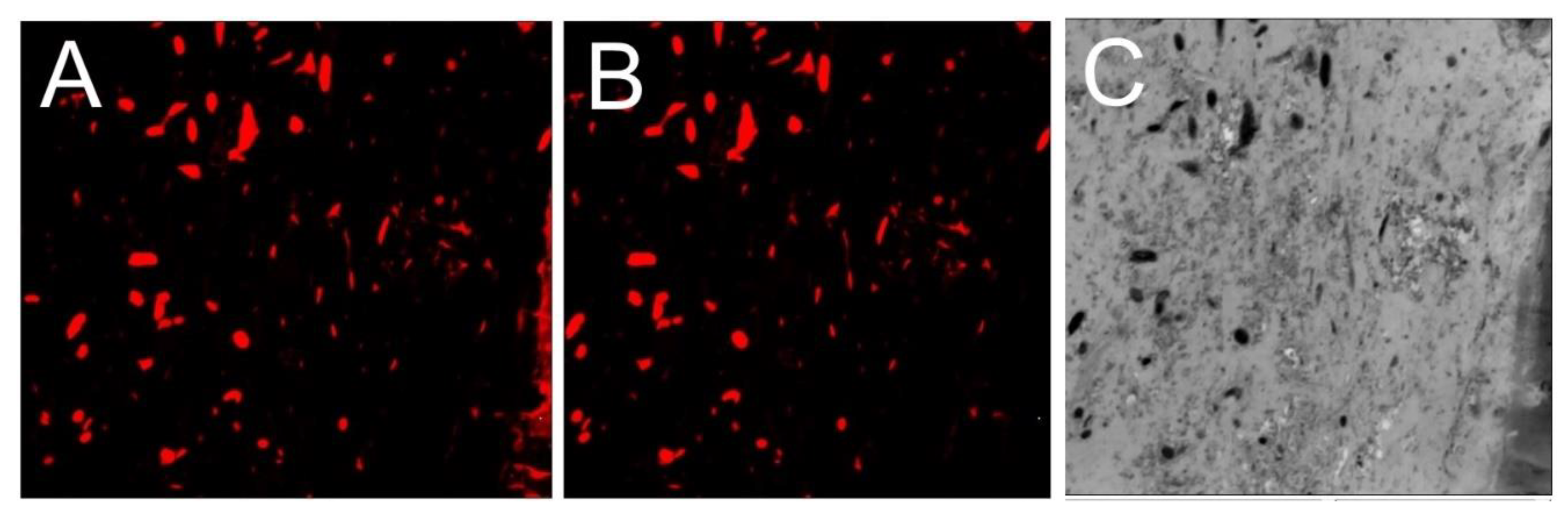
2.3. Digital Image Analysis

Image analysis (Figure 3) was performed using open-source software. A detailed protocol on the individual steps of the image analysis can be found in the Supplementary Material S2. We used the following software: GIMP [18], Fiji (Fiji Is Just ImageJ) [19], Ilastik [20], Drishti (v.2.6.3, v.2.6.4 and v.2.6.5) [21], MeshLab (release 23.12.2016) [22], and Autodesk^® Meshmixer^TM 3.5 (Autodesk, Inc., San Rafael, CA, USA). We used three different versions of Drishti, as the newer versions unfortunately crashed for this high computing demand operation on our computer.

Preprocessing with GIMP included contrast adjustments and compression to 8-bit grayscale files. Stitching and alignment of the images were not necessary. During the cutting of core RWSS, some larger pieces of reed rhizome became detached from the matrix, leaving a cavity in the core, where “rhizomes” were manually painted onto the images. The number of pixels in one millimeter on the reference scale was measured in Fiji to determine the height and width of the 3D model. Subsequently, images were inverted and cropped.

During transfer from the camera’s SD card to the computer, a series of nine images of core RWSS were lost. As a result, the 3D model covers only the contiguous upper 769 images (36.6 cm). The lower 8.6 cm of the RWSS core were not used.

On the images, fresh (alive) belowground biomass could be recognized as elliptical shapes or short thin lines of a bright yellowish or white color. In image analysis, the classification process in which an image is divided into its constituent parts and background, creating distinct object classes, is called segmentation [23]. Segmentation was carried out semiautomatically on all preprocessed images to separate biomass pixels from peat pixels. We used the Fiji plugin “Trainable WEKA segmentation” (TWS) [24], which is based on the RandomForest algorithm from the machine learning toolkit Waikato Environment for Knowledge Analysis (WEKA) [25].

To train and test the algorithm and its settings, objects and areas in a small number of images were manually classified either as “live roots” or “peat matrix”. Different settings for segmentation with the TWS plugin were tested on small substacks of 20 image files containing images from the start, middle, and end of the two image stacks. All tested settings are listed in Appendix C. After selecting the best setting, an automatic segmentation was computed for the complete data set. The large size of the image stacks (RWSN: 101 images, 310 MB and RWSS: 769 images, 1.97 GB) caused memory errors, in spite of 64 GB RAM. To solve this problem, RWSN was divided into four substacks of 25 (26) images and RWSS was divided into seven substacks of 110 (108) images. Segmentation was performed on each substack, creating both probability maps and classified binary images. The substacks were then merged into complete image stacks for the respective cores.

To reduce noise in the segmented images, a size filter was applied. All objects whose small size did not allow a direct affiliation to corresponding objects in neighboring slices were filtered out. A suitable filter was not available for Fiji, so we used the software Ilastik [20]. Segmentation parameters were optimized for a test stack of 20 images (cf., Appendix D). The threshold size for objects was defined as the area of a circle with a diameter equal to the mean distance between cuts, i.e., the mean slice thickness (cf., Appendix E). All objects smaller than 0.79 mm² (95 pixels) in RWSN and 0.18 mm² (65 pixels) in RWSS were discarded.

Objects that were not belowground biomass, but showed the same image signal included ice from the ice cap added to each core, ice crystals that had formed in air pockets in the cores, as well as stones and gravel. Segmentation included these objects in the class of belowground biomass and they would have to be removed by deleting them individually from the image. Only the ice cap signal was removed from the segmented images with the brush tool in Fiji (Figure 4).

Visualization as a 3D volume was carried out using the software Drishti [21]. 3D models were created from filtered as well as unfiltered data stacks. Volume was rendered and slightly smoothed meshes of the volumes of both cores were created.

Additionally, DrishtiPaint v.2.6.5 was used to manually segment single reed rhizomes in the size-filtered data stack of RWSS and extract them as a separate 3D volume of the reed biomass.

2.4. Volume Measurements

Digital volume measurements on the 3D model of RWSS were carried out using DrishtiPaint v.2.6.3. For comparison with manual volumetric measurements on 3 cm thick peat slabs (see below), the model was divided into 13 substacks of 63 images (=3 cm) each starting at the bottom. Volumes were calculated from the number of voxels multiplied by the defined volume of one voxel in cm³ (Appendix F). Additionally, digital volume measurements were carried out using the Fiji plugin “Analyze particles”.

Roots were washed out of the remaining halves of the sample cores. Samples of 3 cm thickness (Appendix G) were washed over a series of four sieves to obtain six subsamples, viz., gravel (>2 mm), sand (0.063–2 mm), rhizomes, living roots with a diameter larger than 2 mm (coarse roots), living roots with a diameter between 2 mm and 1 mm (fine roots), living roots with a diameter smaller than 1 mm (extra fine roots). For each fraction fresh, undecomposed roots and rhizomes were separated manually from detritus. Texture and color of cross-sections were used to identify fresh roots; objects that were dark brown or black instead of white or yellowish in cross-section and which easily fell apart were discarded. In the fractions that were smaller than 1 mm, roots and detritus particles could not always be reliably separated and the smaller root fractions were likely to be slightly overestimated. All lateral roots smaller than 1 mm in diameter were removed with tweezers. The volumetric measurements for all samples were carried out with a Hubbard pycnometer (cf., Appendix H).

3. Results

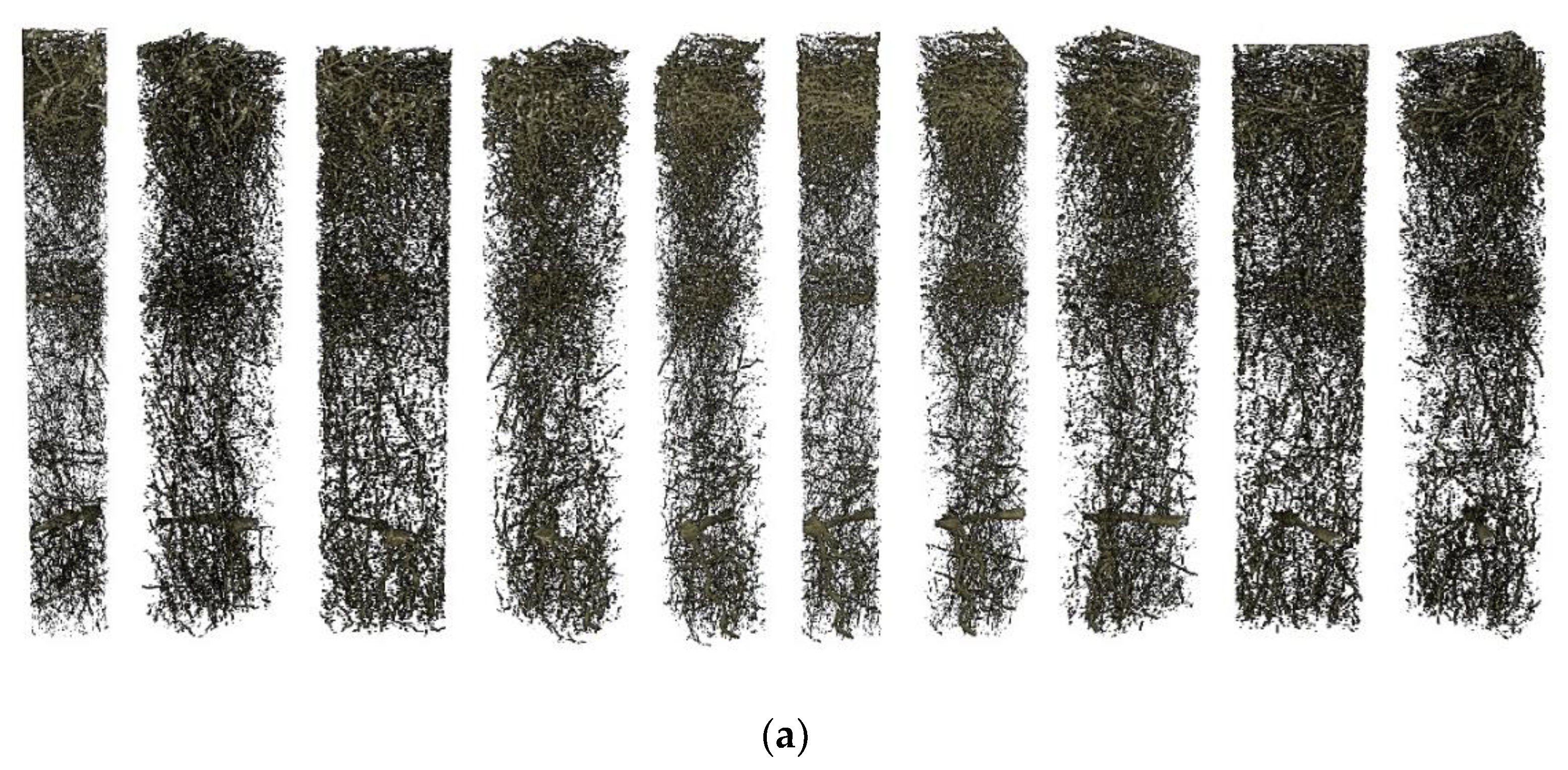
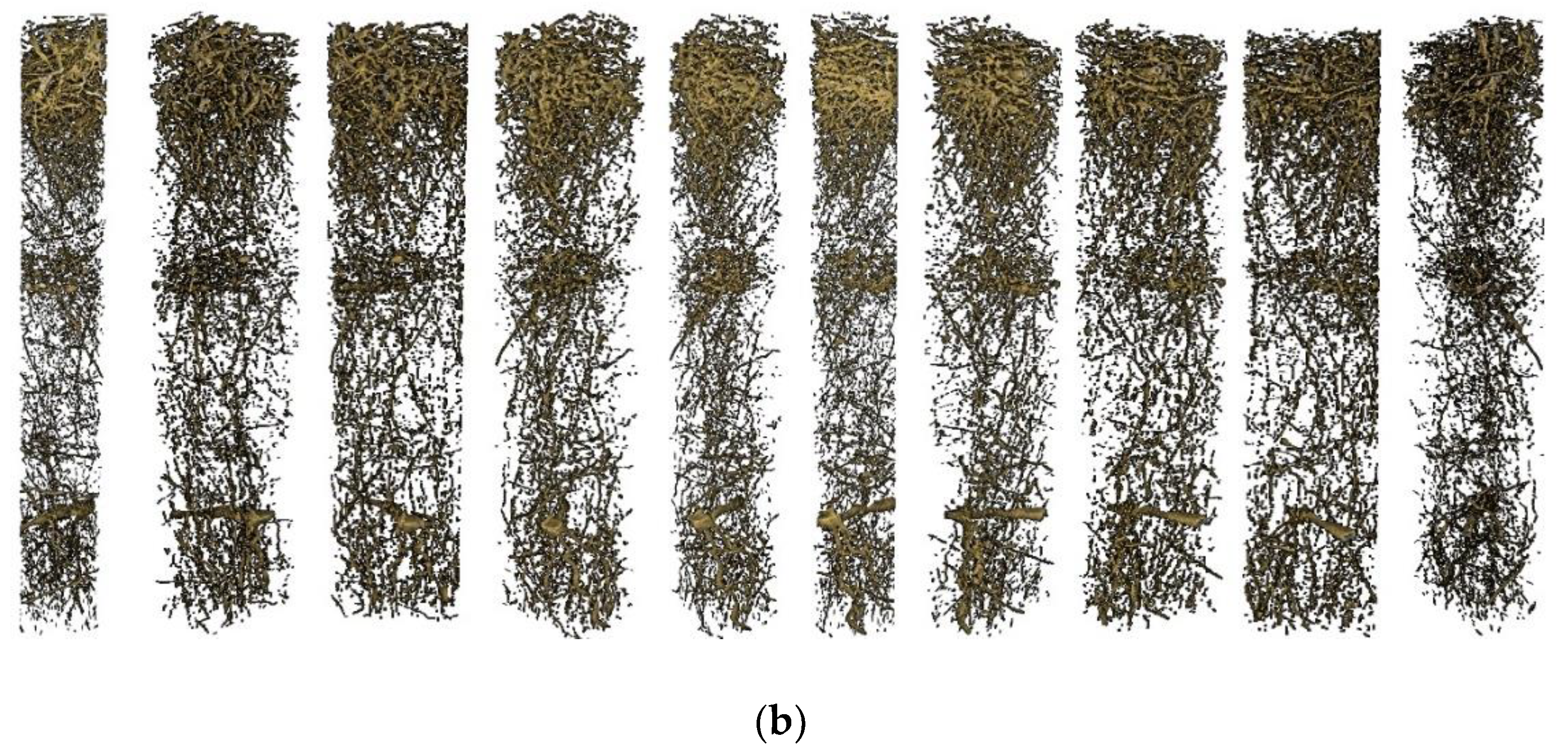
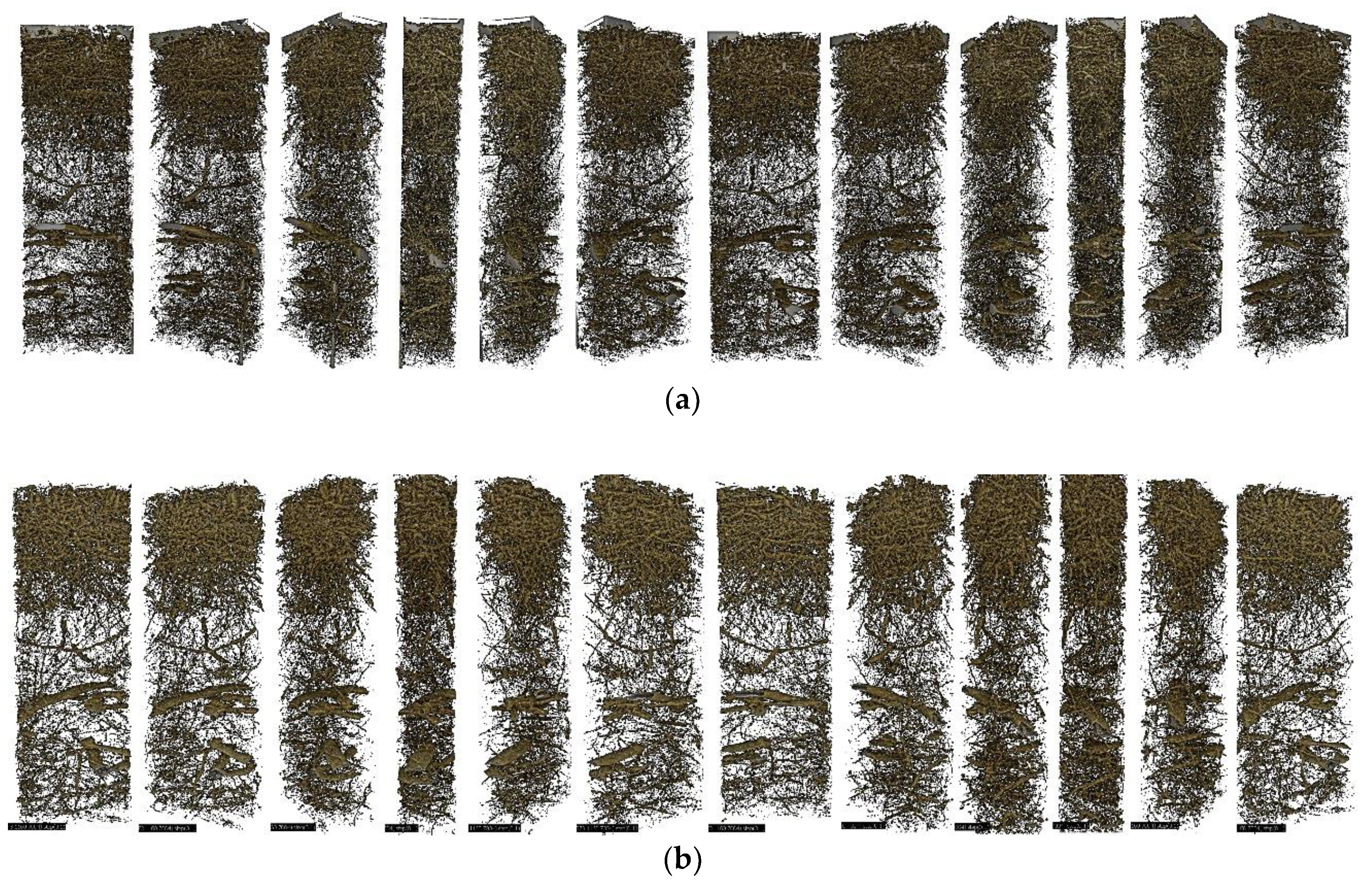
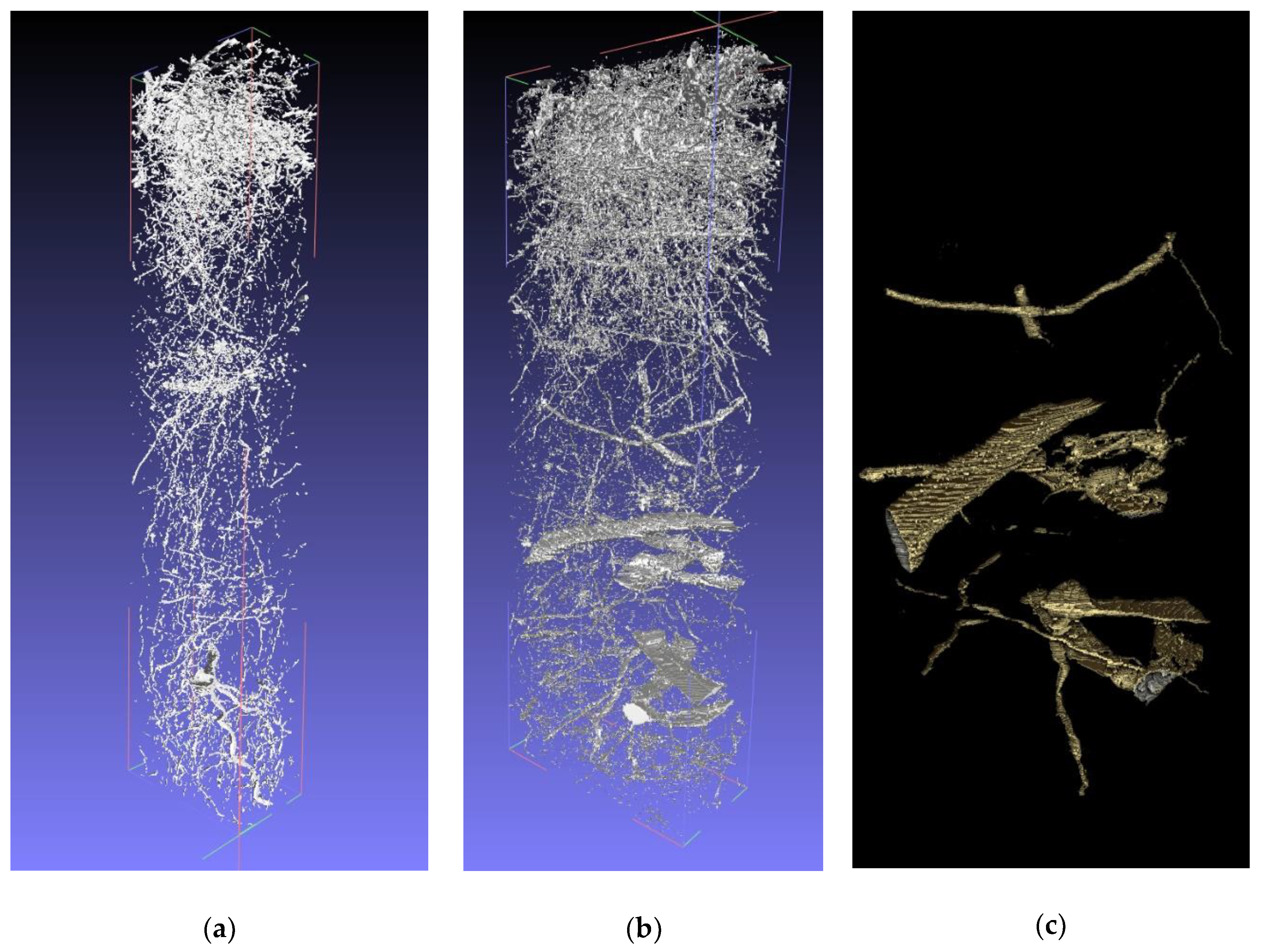
3.1. 3D Model Visualization

Using DAMOCLES and simple photo set-ups, both lengthwise and crosswise sampling generated coherent, reflection-free image data sets which enabled meaningful segmentation and 3D models. The 3D visualizations show dense belowground biomass near the top of the profiles (Figure 5 and Figure 6). Further down rooting is less dense, although somewhat denser layers can be seen in both cores. Applying the size filter and (manual) removal of ice creates a clearer picture of the roots (Figure 5b or Figure 6b). Meshes of the size filtered 3D models were successfully made for RWSN and RWSS without ice (Figure 7a,b). In RWSS large reed rhizomes were found between 22 and 31 cm depth (Figure 7c). Movies of rotating models can be found in the Supplementary Material S3–S6.

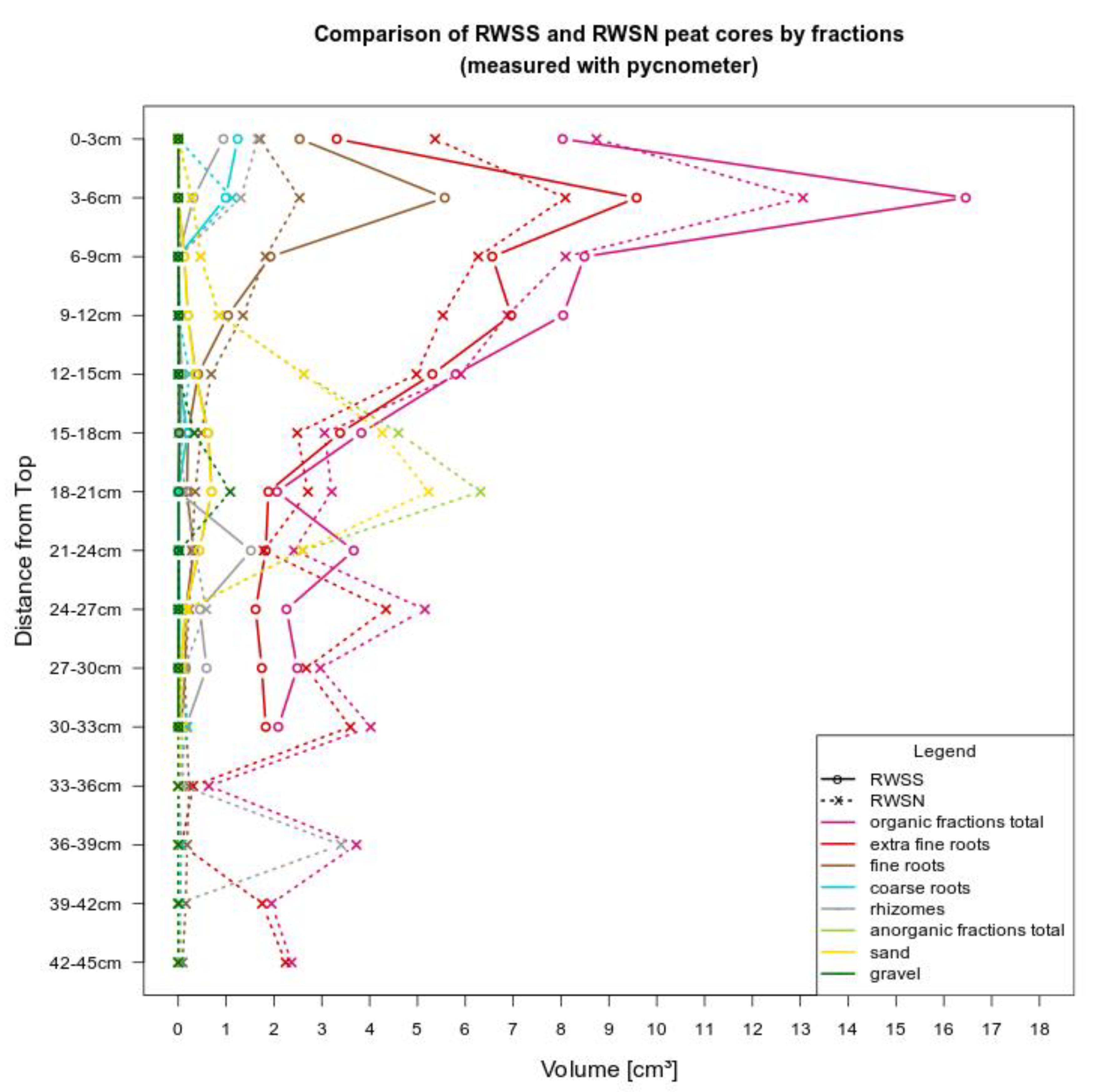
3.2. Volumetric Measurements

3.2.1. Manual Root Washing

Manual root washing showed highest amounts of belowground biomass in the upper 15 cm below the surface in both profiles. The uppermost sample mostly consisted of litter and has lower amounts of roots than the sample below (Figure 8). After this maximum, the total root content decreases steadily to a depth of 18 cm, after which the volume fluctuates. The extra fine roots represent the largest proportion of total roots in both cores. Extra fine roots as well as fine roots are strongly correlated between both cores (Pearson’s r = 0.867 for extra fine roots and r = 0.921 for fine roots). The correlation refers only to depth levels for which data could be acquired in both cores (0–33 cm). Rhizomes are found in RWSN and RWSS in the upper 6 cm, and then appear again below a depth of 21 cm. While the total mineral fraction in the two cores varies greatly, sand is strongly correlated between RWSN and RWSS (Pearson’s r = 0.98).

3.2.2. Model Measurements

Three-dimensional model measurements of root volume were only carried out for RWSS. Ice removal accounts for largest volumetric differences between the filtered and unfiltered models (Figure 9a,b). The 3D models with and without ice removed are strongly correlated (Pearson’s r = 0.864).

Comparison of the volume calculated from the RWSS 3D model (size filtered, without ice) with the volumes obtained by manual washing shows a clear, but not very strong correlation (Figure 10).

4. Discussion

4.1. Technical Aspects

In general, the model represents the distribution of belowground biomass well, with the exception of the litter layer. Extra fine roots with a diameter smaller than 1 mm are not covered by the model at all and parts of the fine roots fraction are underestimated.

In both cores, a substantial amount of sand and gravel was found with highest values between 18 cm and 21 cm. It caused dents and notches on the DAMOCLES blade, which not only made resharpening necessary, but left grooves on the cut surface that showed as parallel white lines in the images. The majority of these lines were filtered out by the size filter, but some were classified as fresh roots. A manual removal of the lines could also be achieved, but would have taken lots of time. It is therefore not recommended to use this method for peat known to have high mineral content, as it would entail considerable additional costs and time.

The lengthwise cutting of RWSN met substantial difficulties. Since the cut had to be made over a large length (44.6 cm), great force was needed. Additionally, the core was deformed during cutting as it repeatedly got stuck under high pressure between the blade and the pushing block, which increased its height. The original image of cut 101 is 77 pixels higher than the original image of cut 1. This increase of 6.5 mm in height had to be removed by cropping from the input image stack for segmentation. Although it is only minor, the cutting process thus added a distortion to the final model. Tests have shown that with lengthwise cutting, the minimum cutting thickness is 1 mm. Yet, a cutting thickness of 1 mm is too large for the creation of the 3D model, as there are gaps in many roots between the cuts and few continuous structures are visible in the 3D model. Moreover, the lengthwise positioning of the core in DAMOCLES led to unevenly illuminated image data. In conclusion, lengthwise cutting of the cores, as well as a slice thickness of 1 mm, is unsuitable for 3D imaging.

The crosswise cutting technique used for RWSS proved well suited for image acquisition. Sectioning could be carried out without any problems and the nominal section thickness of 0.5 mm could well be maintained. The average section thickness deviated only 0.02 mm from the target value. The resulting images were evenly illuminated, which enabled uniform segmentation. Although the number of cuts and thus the time required was considerably higher with crosswise cutting than with lengthwise cutting, it provided more precise image data in which the error due to deformation of the core was much smaller.

In general, the lower the cutting thickness, the more precise the model. Yet, even the relatively small voxel depth of 0.48 mm was not sufficient to represent continuous very fine root structures. Extra fine roots and probably also sand and gravel in both peat cores result in a “voxel cloud” of small disjointed objects. This cloud obstructs observation of larger objects in the center of the 3D models. Therefore, the application of a size filter that removes small disjointed objects is essential.

The large size of the image files led to numerous problems with memory capacity during calculation processes in image analysis. So, either stronger compression or the use of hardware with (even) larger memory capacity is recommended. Workflow was strongly impacted by the fact that only partial stacks of image data could be segmented automatically. The generation of substacks and their subsequent merging required a considerable amount of time, but this problem could be solved through direct scripting in Fiji or Ilastik.

Image acquisition and image segmentation are the most time-consuming steps of the entire method (image acquisition RWSS: 30 h, segmentation RWSS: 10 h). The visualization of the 3D model and volume rendering, as well as the creation of meshes and image output can be carried out in a few hours.

4.2. Volumetric Measurement Methods

Manual washing and sieving allow for directly dividing material into several subclasses, and a large part of the extra fine root fraction can be sampled. However, in our experience the classification of detritus, mineral content, root classes, and rhizomes can vary greatly between individual persons. The assessment of whether an object is a fresh (living) or already dead belowground vascular plant part is very difficult. Rhizomes are especially challenging to classify, as there is a smooth transition between dead and live plant parts. The error of manual classification is therefore not systematic, which weakens the reliability of the results.

The extra fine root fraction likely included relatively much detritus. This error is difficult to quantify as it is not possible to take a representative subsample from the very heterogeneous material for microscopic analysis. Overall, manual sieving and washing techniques can be regarded as prone to errors [7]. Plus, they do not provide insight in the actual structure of the root system.

Compared to the more traditional root washing methods, a major advantage of digital volume measurements is their reproducibility. Segmentation can be performed with different segmentation parameters many times on the same input image data allowing for a comparison of different classifications. For segmentation of the whole image stack (i.e., the entire length of the core), the error is systematic and constant for each image slice. Consequently, any potential error is systematic, which allows for a very good comparison of different input data sets (i.e., cores). Once image data have been generated and segmentation has been performed, digital volume measurements can be performed extremely quickly.

A disadvantage of the digital volume measurements lies in the increased risk of overestimating the volume. A slight overestimation of the outlines of larger roots and rhizomes (i.e., adding a few pixels) during segmentation can lead to large changes in volume, as the circumference for almost circular cross-sections causes a squared increase of the area. Additionally, volume calculations could only be carried out for one class (belowground biomass), as the segmentation was not suited to differentiate between different types of biomass such as rhizomes, coarse roots or fine roots, and even included mineral particles.

Besides close to the surface, there are two deeper layers with high values of extra fine roots in RWSN (Figure 8). These peaks could be associated with reed rhizomes at depth levels 24–27 and 36–39. The 3D models for RWSN and RWSS show many coarse roots growing from reed rhizome nodes into deeper strata (Figure 5 and Figure 6). Fine roots could branch off and lead locally to extra fine root clusters in strata below reed rhizomes. Reed rhizomes occur in RWSS between 21 and 30 cm. In RWSN they are found at comparable depth (24–27 cm), but the largest measured volume of rhizomes in RWSN was found at a depth of 36–39 cm—Reed rhizomes apparently grew at two different depths at the site.

Comparisons between manually measured volumes and the volume derived from the 3D model were only made for the better model derived from the thinner slices. Due to its expansion during freezing, the frozen half of the core (36.6 cm) was about 10% longer than the thawed half (33.4 cm). Considering the uneven surface of the core, there may have been minor differences in length before freezing. No correction was attempted, because the exact depths where expansion took place are unknown. In a future application of the method, inaccuracies in depth layers could be avoided by cutting the core for manual root washing and sieving in a frozen state with DAMOCLES as well. Sectioning would also be more precise, but working time would increase considerably, as preprocessing with a pruning saw is necessary for DAMOCLES. The excess length of the 3D model RWSS (size filtered, without ice) was put at the bottom end of the core. This approach seems valid given the rather large slices and the fact that the peak in “fine roots, coarse roots, and rhizomes” at 21–24 cm is at the same depth in the 3D model.

Actually, the graphs of fine roots, coarse roots, and rhizomes are very similar to the model curve (Figure 10). The only exception is near the top, where the model does not distinguish between roots, rhizomes, and litter, but litter was excluded from the pycnometer measurements.

The correlation of the two curves (volume of fine roots, coarse roots, and rhizomes vs. model volume) is relatively high (r = 0.67, Figure 10). Down to a depth of 12–15 cm the modeled volume is consistently smaller than the volume measured with the pycnometer, in deeper layers it is larger. As these two approaches were done on neighboring but not the same soil volume, this could reflect true differences in root depth distribution. However, it is unlikely that the distribution of roots and rhizomes in this upper part of RWSS varied so much between the two halves of the core, because the difference between RWSN and RWSS (2 m distance) was even smaller (cf., Figure 8).

Apparently, not all roots from the fine roots fraction (1–2 mm) have been modeled. Next to extra fine roots, fine roots represent the largest proportion of the belowground biomass in the upper part of the core (see Appendix I, note that extra fine roots are not included in the 3D model). In contrast, the large peak in the modeled volume at 21–24 cm is mostly absent in the washout, which is likely due to heterogeneity between the two core halves. In the model, large reed rhizomes can be seen at this depth, which were simply absent from the other half.

The modeled volume seems to contain part of the sand. An increase in the modeled volume in 15–18 cm and in 18–21 cm depth lacks correspondence in washed out roots, but does coincide with an increase in the washed out sand.

Davey et al. [7] developed a method similar to the one applied here, in which CT imaging was used to examine the distribution of live coarse roots and rhizomes in peat marsh soils. Similar to the results of this work, roots with a diameter of less than 1 mm (defined as fine roots [7]) could not be detected by CT scans. The CT-based volume determination [7] is more differentiated than the method developed here, as it allows for a distinction between belowground plant biomass and peat as well as mineral constituents. Yet, the CT data are much less precise, because there is a relatively large overlap of the X-ray attenuation signals and no unambiguous classification can be made for large parts of the signals.

In general, the model represents the distribution of belowground biomass well, with the exception of the litter layer. Extra fine roots with a diameter smaller than 1 mm are not covered by the model at all and parts of the fine roots fraction are underestimated.

4.3. 3D Structure

A 3D visualization provides detailed information on the in situ spatial patterns of the root system, which washing out of the roots cannot provide. Metsavainio [12] pinned peat cores to nail boards to fix the spatial pattern of root systems during washing, but this approach only provides a very rudimentary insight into the shape of root systems. Whether the CT imaging approach of Davey et al. [7] (see above) would be suitable for the creation of a 3D model is unclear, because 3D modeling depends on sharp meaningful thresholds between the different fractions, which CT cannot provide. Manual washing is still the only method to determine at least part of the volume of extra fine roots (<1 mm diameter). To what extent the CT data would be suitable for the creation of a 3D model is unclear, because 3D modeling depends on meaningful thresholds between the different fractions. A statistical approach may be opportune, which defines relative contributions of normally distributed, overlapping attenuation signals. Such an approach would, however, likely result in 3D objects with fuzzy edges.

4.4. Applications

Rooting depth and distribution determine peat formation in sedge peats that to a large extent consist of dead root material. The location of root growth determines displacement of the old peat matrix and root degradation provides potential new peat.

A more detailed evaluation of the image data can provide additional information on the heterogeneity of belowground biomass in different depth levels. Statistical methods can be used to analyze the spatial pixel distribution for each image, thus providing insight into spatial distribution of roots and rhizomes. Examples are the application of pixel co-occurrence matrices or simple correlation length assessment that quantifies “clumpiness” relative to a random (homogenous) distribution.

While a large homogeneity can be assumed for the dense root mat in the first nine centimeters of depth, the 3D models indicate a strongly heterogeneous root distribution further below. Such heterogeneity could be caused by uneven nutrient availability [26], by oxygen in the peat soils, or by internal structural barriers such as compaction layers, all of which are in turn affected by root growth. Studying the heterogeneity of the root system can provide insight into the way existing peat is displaced, or hotspots of microbial activity.

The method offers options for in situ studies on competition between species growing in organic soils. If root systems could be assigned to individual plants, characteristic features (volume, length, angle) of the root systems could be measured in the presence or absence of other species.

In addition, the adaptation of root systems under competitive conditions to different environmental factors such as a decrease in water table could be studied in situ. In general, the applied image analysis method still offers potential for improvement. The segmentation could be designed to include more detail by creating different subclasses of belowground biomass similar to the manual method.

We sampled two different cores to compare different working techniques for image acquisition. However, for an improved, more complete view on root architecture, we advise taking several cores for better comparisons.

The analysis of RGB images instead of grayscale images is unlikely to yield improvements for the segmentation, as pixel color values do not differ noticeably between different belowground plant structures, ice, and mineral constituents. The size and shape of the objects seem to be more distinctive. A size filter could be applied here to perform a second segmentation of the images, in which different size classes are distinguished.

5. Conclusions

We provide detailed instructions to create 3D models of belowground plant biomass in peat cores that provide useful insight into the distribution and shape of roots and rhizomes. The distribution of root material derived from the models compares well with manual washouts, but in addition provides spatial information on root structure which is difficult to attain with traditional methods. The method and protocol provided here will, e.g., allow analysis of root responses to nutrient availability, or within and between species competition both within pots or in the field.

References

1. Joosten, H.; Sirin, A.; Couwenberg, J.; Laine, J.; Smitz, P. The Role of Peatlands in Climate Regulation. In Peatland Restoration and Ecosystem Services: Science, Policy and Practice; Bonn, A., Allot, T., Evans, M., Joosten, H., Stoneman, R., Eds.; Cambridge University Press: Cambridge, UK, 2016; pp. 63–76. [Google Scholar]
2. Moen, A.; Joosten, H.; Tanneberger, F. Mire diversity in Europe: Mire regionality. In Mires and Peatlands in Europe—Status, Distribution and Conservation; Joosten, H., Tanneberger, F., Moen, A., Eds.; Schweizerbart Science Publishers: Stuttgart, Germany, 2017; pp. 97–172. [Google Scholar]
3. Grosse-Brauckmann, G. Analysis of vegetative plant macrofossils. In Handbook of Holocene Palaeoecology and Palaeohydrology; Berglund, B.E., Ralska-Jasiewiczowa, M., Eds.; Wiley: Berlin/Heidelberg, Germany, 1986; pp. 591–618. [Google Scholar]
4. Couwenberg, J.; DeKlerk, P.; Endtmann, E.; Joosten, H.; Michaelis, D. Hydrogenetische Moortypen in der Zeit—Eine Zusammenschau. In Landschaftsökologische Moorkunde, 2nd ed.; Succow, M., Joosten, H., Eds.; Schweizerbart Science Publishers: Stuttgart, Germany, 2001; pp. 399–403. [Google Scholar]
5. Pagès, L.; Vercambre, G.; Drouet, J.L.; Lecompte, F.; Collet, C.; Le Bot, J. Root Typ: A generic model to depict and analyse the root system architecture. Plant Soil 2004, 258, 103–119. [Google Scholar] [CrossRef]
6. Hodson, M.J.; Bryant, J.A. Roots. In Functional Biology of Plants, 1st ed.; Hodson, M.J., Bryant, J.A., Eds.; John Wiley & Sons, Ltd.: Chichester, UK, 2012; pp. 124–144. [Google Scholar]
7. Davey, E.; Wigand, C.; Johnson, R.; Sundberg, K.; Morris, J.; Roman, C.T. Use of computed tomography imaging for quantifying coarse roots, rhizomes, peat, and particle densities in marsh soils. Ecol. Appl. 2011, 21, 2156–2171. [Google Scholar] [CrossRef] [PubMed]
8. Taylor, H.M.; Upchurch, D.R.; McMichael, B.L. Applications and limitations of rhizotrons and minirhizotrons for root studies. Plant Soil 1990, 129, 29–35. [Google Scholar] [CrossRef]
9. Busch, J.; Mendelssohn, I.A.; Lorenzen, B.; Brix, H.; Miao, S. A rhizotron to study root growth under flooded conditions tested with two wetland Cyperaceae. Flora Morphol. Distrib. Funct. Ecol. Plants 2006, 201, 429–439. [Google Scholar] [CrossRef]
10. Kokkonen, P. Beobachtungen über das Wurzelsystem der Kiefer im Moorböden. Acta For. Fenn. 1923, 25, 1–21. [Google Scholar] [CrossRef]
11. Rigg, G.B.; Harrar, E.S. The root systems of trees growing in sphagnum. Am. J. Bot. 1931, 18, 391–397. [Google Scholar] [CrossRef]
12. Metsävainio, K. Untersuchungen über das Wurzelsystem der Moorpflanzen. Annales Botanici Societatis Zoologicae-Botanici Fennici Vanamo 1931, 1, 1–422. [Google Scholar]
13. Kettridge, N.; Binley, A. X-ray computed tomography of peat soils: Measuring gas content and peat structure. Hydrol. Process. Int. J. 2008, 22, 4827–4837. [Google Scholar] [CrossRef]
14. Kettridge, N.; Binley, A. Characterization of peat structure using X-ray computed tomography and its control on the ebullition of biogenic gas bubbles. J. Geophys. Res. Biogeosci. 2001, 116. [Google Scholar] [CrossRef]
15. Gharedaghloo, B.; Price, J.S.; Rezanezhad, F.; Quinton, W.L. Evaluating the hydraulic and transport properties of peat soil using pore network modeling and X-ray micro computed tomography. J. Hydrol. 2018, 561, 494–508. [Google Scholar] [CrossRef]
16. Clymo, R.S. A high-resolution sampler of surface peat. Funct. Ecol. 1988, 2, 425–431. [Google Scholar] [CrossRef]
17. Joosten, H.; DeKlerk, P.D. DAMOCLES: A DAshing MOnolith Cutter for fine sectioning of peats and sediments into LargE Slices. Boreas 2007, 36, 76–81. [Google Scholar] [CrossRef]
18. GIMP. GNU Image Manipulation Program. Available online: www.gimp.org (accessed on 13 January 2020).
19. Schindelin, J.; Arganda-Carreras, I.; Frise, E.; Kaynig, V.; Longair, M.; Pietzsch, T.; Preibisch, S.; Rueden, C.; Saalfeld, S.; Schmid, B.; et al. Fiji: An open-source platform for biological-image analysis. Nat. Methods 2012, 9, 676–682. [Google Scholar] [CrossRef] [PubMed] [Green Version]
20. Sommer, C.; Straehle, C.; Koethe, U.; Hamprecht, F.A. Ilastik: Interactive learning and segmentation toolkit. In Proceedings of the 2011 IEEE International Symposium on Biomedical Imaging: From Nano to Macro, Chicago, IL, USA, 30 March–2 April 2011; IEEE: New York, NY, USA, 2011; pp. 230–233. [Google Scholar] [CrossRef]
21. Limaye, A. Drishti: A volume exploration and presentation tool. In Developments in X-Ray Tomography VIII; SPIE: Washington, DC, USA, 2012; p. 85060X. [Google Scholar] [CrossRef] [Green Version]
22. Cignoni, P.; Callieri, M.; Corsini, M.; Dellepiane, M.; Ganovelli, F.; Ranzuglia, G. Meshlab: An open-source mesh processing tool. In Proceedings of the Eurographics Italian Chapter Conference, Salerno, Italy, 2–4 July 2008; pp. 129–136. [Google Scholar]
23. Bengtsson, E.; Wahlby, C.; Lindblad, J. Robust cell image segmentation methods. Pattern Recognit. Image Anal. C/c Raspozn. Obraz. Anal. Izobr. 2004, 14, 157–167. [Google Scholar]
24. Arganda-Carreras, I.; Kaynig, V.; Rueden, C.; Eliceiri, K.W.; Schindelin, J.; Cardona, A.; Sebastian Seung, H. Trainable Weka Segmentation: A machine learning tool for microscopy pixel classification. Bioinformatics 2017, 33, 2424–2426. [Google Scholar] [CrossRef] [PubMed]
25. Hall, M.; Frank, E.; Holmes, G.; Pfahringer, B.; Reutemann, P.; Witten, I.H. The WEKA data mining software: An update. ACM SIGKDD Explor. Newsl. 2009, 11, 10–18. [Google Scholar] [CrossRef]
26. Hodge, A.; Berta, G.; Doussan, C.; Merchan, F.; Crespi, M. Plant root growth, architecture and function. Plant Soil 2009, 321, 153–187. [Google Scholar] [CrossRef]
Figure 1. Preparation of the peat monolith: (a) Shape of the monolith before and after size adjustment. (b) Creation of the ice cap—an acrylic glass plate was positioned a few centimeters away from the plant and litter surface at a 90° angle to the sides of the core; it was attached to tinfoil that was then pressed firmly against the frozen peat. The core was placed in the freezer (−18 °C) and precooled water (+4 °C) was poured into the gap in 10 mL units for every 30 min until it was filled up entirely with ice.
Soilsystems 04 00013 g001
Figure 2. Cutting with DAMOCLES [17] (p. 77, modified).
Soilsystems 04 00013 g002
Figure 3. Workflow diagram of the image analysis with open-source software.
Soilsystems 04 00013 g003
Figure 4. Ice removal using Fiji: (A) Upper section of probability map for RWSN, slice 88. Ice (lower right corner) is included in the segmentation. (B) Same section after manual ice removal. (C) Image of the same section before segmentation for comparison. Belowground biomass is displayed in dark pixels hues, as the image is inversed.
Soilsystems 04 00013 g004
Figure 5. Image series of 3D model for RWSN rotating clockwise. (a) Unfiltered and with ice on top, (b) with size filter and ice removed. The size of the monolith is 6.0 cm × 10.1 cm × 44.6 cm.
Soilsystems 04 00013 g005aSoilsystems 04 00013 g005b
Figure 6. Image series of 3D model for RWSS rotating clockwise. (a) Unfiltered and with ice on top, (b) with size filter and ice removed. The size of the monolith is 6.1 cm × 12.5 cm × 36.6 cm.
Soilsystems 04 00013 g006
Figure 7. (a) Mesh of 3D model RWSN (size filtered with ice removed), (b) mesh of 3D model RWSS (size filtered with ice removed), (c) 3D model of reed rhizomes extracted from model RWSS (size filtered with ice removed).
Soilsystems 04 00013 g007
Figure 8. Volume (per cm depth) of washed out root and clastic fractions in RWSN and RWSS as measured with a pycnometer.
Soilsystems 04 00013 g008
Figure 9. Volume per slice (0.48 mm) for the 3D model of RWSS as measured in Fiji. (a) Size filtered model without ice. (b) Unfiltered model with ice.
Soilsystems 04 00013 g009
Figure 10. Drishti volume calculations (RWSS with size filter and ice removed) and pycnometer measurements.
Soilsystems 04 00013 g010