A Review of the Science and Logic Associated with Approach Used in the Universal Soil Loss Equation Family of Models

Abstract

Soil erosion caused by rain is a major factor in degrading agricultural land, and agricultural practices that conserve soil should be used to maintain the long-term sustainability of agricultural land. The Universal Soil Loss Equation (USLE) was developed in the 1960s and 1970s to predict the long-term average annual soil loss from sheet and rill erosion on field-sized areas as an aid to making management decisions to conserve soil. The USLE uses six factors to take account of the effects of climate, soil, topography, crops, and crop management, and specific actions designed to conserve soil. Although initially developed as an empirical model based on data from more than 10,000 plot years of data collected in plot experiments in the USA, the selection of the independent factors used in the model was made taking account of scientific understanding of the drivers involved in rainfall erosion. In addition, assumptions and approximations were needed to make an operational model that met the needs of the decision makers at that time. Those needs have changed over time, leading to the development of the Revised USLE (RUSLE) and a second version of that, the Revised USLE, Version 2 (RUSLE2). While the original USLE model was not designed to predict short-term variations in erosion well, these developments have involved more use of conceptualization in order to deal with the time-variant impacts of the drivers involved in rainfall erosion. The USLE family of models is based on the concept that the “unit” plot, a bare fallow area 22.1 m long on a 9% slope gradient with cultivation up and down the slope, provides a physical situation where the effect of climate and soil on rainfall erosion can be determined without the need to consider the impact of the four other factors. The science and logic associated with this approach is reviewed. The manner by which the soil erodibility factor is determined from plot data ensures that the long-term average annual soil loss for the unit plot is predicted well, even when the assumption that event soil loss is directly related to the product of event rainfall energy, and the maximum 30-min intensity is not wholly appropriate. RUSLE2 has a capacity to use CLIGEN, the weather generator used in WEPP, and so can predict soil losses based on individual storms in a similar way to WEPP. Including a direct consideration of runoff in determining event erosivity enhances the ability to predict event soil losses when runoff is known or predicted well, but similar to more process-based models, this ability is offset by the difficulty in predicting runoff well.

1. Introduction

Soil erosion caused by rain is a major factor in degrading agricultural land, and the agricultural practices that conserve soil should be used to maintain the long-term sustainability of agricultural land. The Universal Soil Loss Equation (USLE) [1,2] was developed to predict the long-term (~20 years) average annual soil loss (A, mass/unit area/year) from sheet and rill erosion on field-sized areas as an aid to making management decisions to conserve soil. The USLE uses six factors:

A = R K L S C P

(1)

where R is the climatic factor normally referred to as the rainfall “erosivity” factor, K is the soil “erodibility” factor, L is the slope length factor, S is the slope gradient factor, C is the crop and crop management factor, and P is the soil conservation practice factor. It is an empirically-based model that was originally developed from runoff and soil loss experiments using field plots under natural rainfall at 10 experiment stations set up after 1929 in the USA to demonstrate the effect of soil conservation practices. The initial development of mathematical equations to estimate soil losses caused by rainfall and the impact of alternate practices did not begin until the 1940s. The main work on developing the USLE began in the mid 1950s, many years before the USLE model was fully described in USDA Agricultural Handbook 282 published in 1965 [1]. The USLE was later revised (RUSLE) [3], in which the mathematical operation of the model was retained, but the manner by which some of the factors were determined was changed based on new research undertaken since the mid-1960s.

The USLE/RUSLE model is widely used to predict rainfall erosion throughout the world. Although it is apparent from Equation (1) that the focus is the prediction of long-term average annual soil losses, erosion varies in time and space in the short term, and the USLE approach needs to make provision for this. Consequently, the factors in the Universal Soil Loss Equation family of models are not only described, but the science and logic associated with them are also reviewed in this paper. In addition, the performance of USLE-based technology is compared with the performance of WEPP [4], the more physically-based model developed as an alterative to using the RUSLE in the USA.

2. The USLE/RUSLE Model Factors

Zingg [5] published the results of a comprehensive study on the effects of slope steepness and slope length on erosion from runoff and soil loss plots in the USA. This was followed in 1941 by Smith, who added cropping and support practice factors to Zingg’s function. By the late 1950s, over 10,000 plot years of data had been collected, and together with Smith, Wischmeier developed the mathematical structure described in Equation (1).

As noted above, the runoff and soil loss plots that provided the data for the USLE were originally set up to demonstrate the effect of soil conservation practices and consequently, the size used for many of the plots was the size commonly used in agronomic experiments, 1/100th of an acre. As a result, many plots were 6 feet (1.8 m) wide and 72.6 feet (22.1 m) long. Plots of other slope lengths did exist. A common approach adopted in agronomy in the 1960s was to compare the effect of a treatment to the results obtained for a “control” plot. Wischmeier and Smith chose the so-called “unit” plot, a bare fallow area 72.6 feet (22.1 m) long cultivated up and down the slope when the slope gradient is 9% as the basis for the USLE. As a consequence of this, the USLE/RUSLE model operates mathematically in two steps. The first step is to predict soil loss from the unit plot (A₁), where L, S, C, and P all have values of 1.0:

A₁= R K

(2)

The second step modifies that value to take account of the conditions that vary from the unit plot.

A = A₁L S C P

(3)

The conditions set for the unit plot are somewhat arbitrary. The unit plot could have been longer or shorter, or on a steeper or less steep slope. However, conceptually, the unit plot provides the physical model on which the USLE is based, and Equation (2) is designed to account for the effect of geographic variations in climate and soil on soil loss. Equation (3) is designed to account for local variations in slope length, gradient, and cropping practices once the effect of climate and soils has been established at a location.

2.1. The R Factor

Equation (2) deals with the effect of geographic variations in soil and climate on erosion caused by sheet and rill erosion. R is defined as the average annual value of the product storm kinetic energy (E) multiplied by the maximum 30-min intensity (I₃₀):

$$R={\displaystyle \sum _{n=1}^N{\left(E{I}_{30}\right)}_n/\gamma }$$

(4)

where N is the number of valid rainfall events in Y years. Rain showers of less than 12.5 mm (0.5 in) were omitted in the calculation of R unless at least 6.25 mm (0.25 in) of rain fell in 15 min. A period of 6 h with less than 1.27 mm (0.05 in) was used as a storm separator. A direct linear relationship between event soil loss from bare fallow and EI₃₀ for runoff producing events was demonstrated to exist at Bethany, Missouri by Wischmeier and Smith [6].

E, storm rainfall energy, was not determined directly, but was usually calculated from rainfall energy–intensity relationships based on the data on raindrop sizes obtained in Washington, DC, by Laws and Parsons [7]. Initially, in the USLE, the energy per unit quantity of rain or unit kinetic energy was determined from a logarithmic relationship with rainfall intensity, the metric version being:

e_m = 0.119 + 0.0873 log₁₀ (i_m),      i_m ≤ 76 mm h⁻¹

(5a)

e_m = 0.283,              i_m > 76 mm h⁻¹

(5b)

where e_m has units of megajoule per hectare per millimeter of rainfall (MJ ha⁻¹ mm⁻¹). The limit of 76 mm h⁻¹ applied to Equation (5a) resulted from observations that Equation (5a) overpredicted e_m when the intensity exceeded that value. In RUSLE [3], Equation (5) was replaced by:

e_m = 0.29 (1 − 0.72 exp (−0.05 i_m))

(6)

where as, in RUSLE2 [8]:

e_m = 0.29 (1 − 0.72 exp (−0.082 i_m))

(7)

As shown by Nearing [9], Equation (7) produces higher e_m values than Equation (6) below i_m = 70 mm h⁻¹ but both Equations (6) and (7) produce little variation in e_m values once i_m exceeds 80 mm h⁻¹.

In reality, storm kinetic energies can vary greatly from the values predicted depending on the synoptic conditions that produce the rainfall [10]. Although the original conceptual model is based on the understanding that raindrop impact is an important factor in supplying the energy required to cause erosion, in using Equations (5) or (6) or (7), the USLE/RUSLE model ignores the actual variations in rainfall kinetic energy that occur in time and space. In effect, these equations emphasize the influence of rain produced at high intensities in comparison to low-intensity rainfall. This emphasis is enhanced further, because I₃₀ is highly influenced by high intensities that are associated with the peak rainfall rate that occurs during a rainstorm.

Although R is assumed not to vary with slope gradient, on low slopes, raindrop impacts tend to be more buffered by water ponded on the surface than on steeper slopes. Consequently, the RUSLE provides an adjustment factor to account for the reduction of R by ponded water on low slopes [3]. In the USLE, storms showers of less than 12.5 mm (0.5 in) were omitted in the calculation of R unless at least 6.25 mm (0.25 in) of rain fell in 15 min. In RUSLE, all storms were considered in the calculation of R in the western regions of the USA. While it was argued that this had little effect on the value of R, the reason why storms less than 12.5 mm were originally omitted was that storms less than 12.5 mm were observed by Wischmeier and Smith to often not produce appreciable amounts of runoff and soil loss and, very importantly, the direct linear relationship between event soil loss from bare fallow and EI₃₀ that was demonstrated to exist at Bethany, Missouri by [6] was determined from only storms that produced runoff and soil loss. In reality, the USLE/RUSLE model is based on:

A_1.e = EI₃₀  K,         Q_e > 0

(8)

where A_1.e = event soil loss (mass/area) from the unit plot, and Q_e (volume/area) is the runoff amount for the event.

Determining EI₃₀ values for individual storms using e_m values requires high-resolution data on the rainfall intensities that occur during a storm. Mapping techniques have been widely used to estimate R values between locations where such data are available [1,2,3,11,12]. However, it should be noted that the amount of soil eroded varies during the year depending on how the erosive rainfall is distributed in time at a location, and how the protective effect of vegetation varies over time. Consequently, in the USLE, not only is R determined using Equation (4), but also the proportion of R that occurs during various crop stages is determined in order to deal with the interaction between rain and vegetation on soil loss. In the RUSLE, the proportion of R that occurs in each half month is used.

2.2. The K Factor

K is the average annual soil loss per unit of R. Originally, K values were determined from runoff and soil loss plot data using:

$$K=\frac{{\displaystyle \sum _{n=1}^N{\left(A_{e.1}\right)}_n}}{{\displaystyle \sum _{n=1}^N{\left(E{I}_{30}\right)}_n}}$$

(9)

It follows from Equation (8) that K replaces the regression coefficient that usually associated a direct linear relationship between event soil loss from the unit plot and EI₃₀. However, Equation (9) ensures that the total soil loss predicted for the set of events used to obtain K is the same as the total of the soil loss observed for that set of events. That is not always the case when K is determined as the regression coefficient in the relationship between event soil loss from the unit plot and EI₃₀.

Given the expense and time necessary to operate appropriate runoff and soil loss plots, methods to predict K from soil properties were developed later [13]. Wischmeier et al. [14] developed a soil erodibility nomograph for determining K from soil properties. A mathematical approximation was then developed [2] for those cases where the silt plus fine sand fraction does not exceed 70%:

K = [2.1 (10⁻⁴) (12 − OM) M^1.14 + 3.25(s − 2) + 2.5(p − 3)]/100

(10)

where M is the percentage of silt (0.02–0.1 mm) multiplied by the quantity of 100% clay, OM is the percentage of organic matter, s is the soil structure code in the US soil classification, and p is the profile permeability class. Auerswald et al. [15] have developed a more precise equation to predict K from soil properties.

Often, in the rainfall simulation experiments undertaken to determine K, artificial rainfall is applied to a plot at about 64 mm hr⁻¹ under natural antecedent soil–water conditions (dry run), followed by a 30-min simulation 4 h later (wet run), and another 30-min simulation 30 min later (very wet run). This approach results in K being calculated from:

K = (13 K_d + 4 K_w + 3 K_vw)/20

(11)

where K_d, K_w, and K_vw are the respective values for the soil erodibilities associated with the dry, wet, and very wet runs [16]. The weighting used in Equation (11) reflects a storm frequency distribution for central USA [17].

In the development of the RUSLE, it was recognized that seasonal variations in soil properties and runoff also resulted in seasonal variations in K. While the pattern for temporally varying erodibility was well defined at some locations, it was not at others. Examination of the RUSLE temporal soil erodibility equations showed that they worked poorly at 11 locations, and were not applicable in the Western USA [8].

In RUSLE2 [8], a version of the RUSLE that uses a daily time step in the calculation of soil loss in the USA, temporal variations in soil erodibility in the USA are calculated using monthly precipitation and temperature as independent variables. In the Eastern USA:

K_j/K_n = 0.591 + 0.732 (P_j/P_s) − 0.324 (T_j/T_s),      T_j ≥ 30 °F

(12a)

K_j/K_n = (K_sj/K_n) exp (−0.2(30 − T_j)),         T_j < 30 °F

(12b)

where K_j is the average daily soil erodibility factor value for the jth day, K_n is the average soil erodibility determined from soil properties, T_j is the average daily temperature for the jth day in Farenheit, T_s is the average daily temperature for the RUSLE2 summer period, P_j is the average daily precipitation in inches, P_s is the daily average precipitation for the summer period, and K_sj is the soil erodibility factor calculated for the jth day using Equation (12). Figure 1 shows how K varies during the year when Equation (12) is applied at Presque Isle, Maine (ME), and Bethany, Missouri (MO) in the USA.

It is important to note that the approach results in the average annual value for soil erodibility calculated from soil properties vary geographically with climate in the USA. However, Equation (12) does not describe increased soil erodibility during or immediately after soil thawing, or work well in the Western USA. In the Western USA, P_s and T_s values are set to the values at Columbia, Missouri to give:

K_j/K_n = 0.591 + 0.732 (P_j/0.123) − 0.324 (T_j/62.8)

(13a)

K_j/K_n = 2.0,         K_j/K_n > 2.0

(13b)

K_j/K_n = 0.4,         K_j/K_n < 0.4

(13c)

This equation estimates increased K values at locations where more precipitation or cooler summers create wetter soil conditions with an increased likelihood of runoff occurring. The applicability of this approach outside the USA is untested.

In many cases where the USLE/RUSLE model has been applied either in the USA or outside the USA, soil erodibilty values are assumed to remain constant with time. Consequently, the USLE/RUSLE model has been frequently applied either in the USA or outside the USA without recognizing that the values of K generated by Equation (10) need to be adjusted for the climate at the location being considered when that location is outside the central USA. However, other equations for calculating K from soil properties have been developed for places such as Hawaii [19], Australia [20], Sicily [21], and elsewhere. Panagos et al. [22] applied Equation (10) with an adjustment for stone cover throughout Europe.

2.3. Alternatives to EI₃₀

The USLE model was designed to predict long-term soil loss. However, given that the USLE is based on Equation (8), it can be applied to predicting soil losses on a shorter time scale. Tiwari et al. [23] observed that the RUSLE overpredicts small average annual soil losses and underpredicts high average annual soil losses in the USA. Although event soil loss from bare fallow was shown to be directly related with event EI₃₀ at Bethany, Missouri by Wischmeier [6], that is not the case for all the geographic locations in the USA. Foster et al. [24] observed that an event erosivity index that had a provision to account for both raindrop and flow-driven erosion separately was better than the EI₃₀ index. Earlier, Williams [25] had proposed the Modified Universal Soil Loss Equation (MUSLE):

R_e = 11.8 (Q_ve q_pe)^0.56

(14)

where R_e is the event erosivity index, Q_ve is the volume of runoff for the event in m³, and q_pe is the peak flow rate for the event in m³ s⁻¹. The focus of the MUSLE is sediment yield from watersheds, where Williams et al. perceived flow-driven erosion to be dominant. It should be noted that the value of 11.8 was empirically derived for the specific conditions used by Williams. It does not necessarily apply to all areas where flow-driven erosion is dominant.

It seems that the MUSLE influenced Onstad and Foster [26] to propose an erosivity index which included a provision to account for both raindrop and flow-driven erosion separately:

R_e = αEI₃₀ + βχQ_e1(q_p)^0.33

(15)

where Q_e1 is the event runoff amount from the unit plot, and α and β are coefficients that add together to make 1.0, and adjust for variations in the relative capacities of rain and runoff to cause erosion. Assumptions have to be made about the relative effects raindrop-driven and flow-driven erosion in order to set the values of α and β when predicting soil loss. Onstad and Foster [26] used α = β = 0.5 and adjusted the value of χ so that it resulted in the average annual average of the value produced by Equation (15) being equal to value of R calculated using EI₃₀ alone. Other indices such as:

R_e = 1.586 (Q_eqpe)^0.56 DA^0.12

(16a)

R_e = 0.65 EI₃₀ + 0.45 (Q_eqpe)^0.33

(16b)

R_e = 2.5 (Q_eqpe)^0.5

(16c)

R_e = 0.79 (Q_eqpe)^0.65 DA^0.009

(16d)

R_e = b₅ Q_e^b4 q_pe^b5 DA^b6

(16e)

where DA is drainage area expressed in ha, and b4–b6 are user-selected coefficients that are used as alternatives to EI₃₀ in APEX [27]. APEX expanded the number of the erosivity index options available in EPIC [28]. Williams et al. [28] also developed an alternative equation to the one used in the USLE to calculate K. When used to model soil loss, Equations (14), (15), (16a)–(16e) all use USLE/RUSLE K values, even though K has units of soil loss per unit of EI₃₀. Equation (15) is the only one that can use USLE/RUSLE Ks legitimately, because χ is set so that the average annual average of the value produced by Equation (15) was equal to the value of R calculated using EI₃₀. USLE/RUSLE Ks have units of soil loss per unit EI₃₀, and that fact needs to be respected when they are used in soil loss prediction models.

Another index that can be considered as an alternative to EI₃₀ is the QE_A index. This index is calculated by summing the product of the runoff rate (Q) and the rainfall kinetic energy flux (E_A) during a rainstorm. Runoff is an important factor in determining event soil loss, not just because of flow-driven erosion, but also because the soil loss from runoff and soil loss plots is directly related to the product of runoff and sediment concentration, as well as the mass of soil per unit of runoff. The QE_A index is based on the concept that sediment concentration varies with the rainfall kinetic flux that is applied when runoff occurs. Kinnell et al. [29] showed that the QE_A index estimated event soil losses from a bare fallow plot at Holly Springs, Mississippi (MS), better than EI₃₀. They also showed that the excess rainfall rate (I_x), which can be determined assuming that the infiltration rate of the soil is constant during the rainstorm, could be used as a surrogate for Q. The coefficients of determination (r²) for the two bare fallow plots at Holly Springs were 0.5173, 0.6429, and 0.6264 on plot C5, and 0.4613, 0.5758, and 0.5758 on plot C7 for EI₃₀, QE_A, and I_xE_A respectively. The lack of available data on runoff rates and rain intensities during rainstorms at other locations prevented examination of the applicability of QE_A and I_XE_A indices at other locations in the USA.

As noted above, runoff is an important factor in determining event soil loss, because soil loss from runoff and soil loss plots is directly related to the product of runoff and sediment concentration (the mass of soil per unit of runoff). When the USLE/RUSLE model is considered in terms of the product of runoff and sediment concentration, it can be seen that the model is based on assumption that the sediment concentration associated with the unit plot varies inversely with runoff:

A_e.1 = Q_e1 (K EI₃₀ Q_e1⁻¹)

(17)

Kinnell and Risse [30] observed that for the bare fallow runoff and soil loss plots in the USLE database, sediment concentration was better related to EI₃₀ per unit quantity of rain than EI₃₀ per unit quantity of runoff. As a result, soil loss for the unit plot predicted by the USLE-M, the name given to the model based on this result, is given by:

A_e.1 = Q_Re.1EI₃₀ K_UM.

(18)

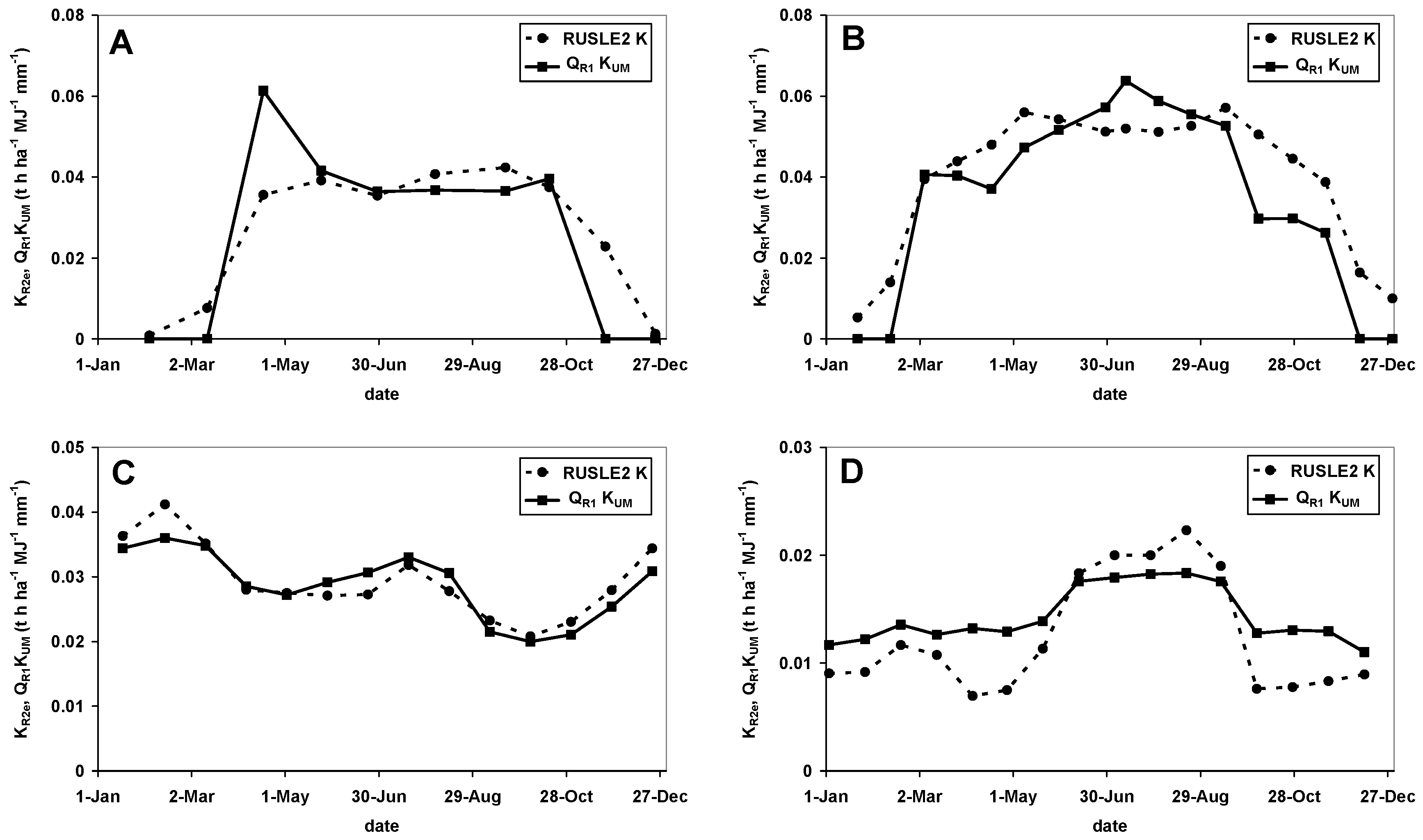
where Q_Re.1 is the runoff ratio for the event from the unit plot, and K_UM is the soil erodibility for the event, which has a different value from K, because the event erosivity index is equal to Q_R1EI₃₀, not to EI₃₀. An example of the improvement in using Equation (18) in place of Equation (8) is shown in Figure 2 when runoff amounts are known, and:

$$K_{UM}=\frac{{\displaystyle \sum _{n=1}^N\left(A_{e.1}\right)n}}{{\displaystyle \sum _{n=1}^N \left(Q_{Re.1}{EI}_{30}\right)n}}$$

(19)

Obviously, the improvement is not as great when runoff is predicted rather than measured. However, the lack of precision provided by runoff prediction methods will influence the ability of any model that includes runoff as a factor in the prediction of soil loss. Physically-based rainfall erosion models such as WEPP [4] use runoff as a factor in the prediction of soil loss from both rill and interrill areas.

Equation (18) can be rewritten as:

A_e.1 = EI₃₀ (Q_Re.1 K_UM)

(20)

It follows from Equation (20) that the product of Q_Re.1 K_UM provides runoff-influenced erodibility values that can used as alternatives to the values of Kj that are normally used in RUSLE2. RUSLE2 has a facility to produce a series of representative storms with associated runoff amounts calculated using the Curve Number (CN) method [32], with empirical equations that vary the values of CN in association with both soil moisture and rainfall intensity [33]. Figure 3 shows how the two different approaches to determining erodibilities for the representative storms compare with each other at four locations in the USA.

The assumption that A_e.1 is directly related to Q_R1EI₃₀ is challenged by data collected from bare fallow runoff and soil loss plots at the Sparacia site in Sicily, Italy. Bagarello et al. [34] observed that event soil losses from the unit plot varied with Q_R1EI₃₀ to a power of 1.61. Subsequent analysis reduced the power to 1.47 [35] and, based on this result, they proposed the model that they called the USLE-MM.

A_e.1 = K_UMM (Q_REI₃₀)^b1

(21)

where b1 > 1 and K_UMM is the soil erodibility factor when (Q_REI₃₀)^b1 is used in place of Q_REI₃₀. For the Masse site in Umbria, Italy, they observed the power to be 1.16 [36]. Bagarello et al. [36] provided no substantiated physical reason why the power of the Q_R1EI₃₀ index should be greater than 1.0 at these two locations. For the USA data used by Kinnell and Risse [30], powers were mainly grouped within the range of 0.73 to 1.05 [37]. The exceptions were plots 1–2 at Tifton, Georgia, where the power was 0.419. No physical explanation is available for these values.

In the USLE-MM, K_UMM is given by:

$$K_{UMM}=\frac{{\displaystyle \sum _{n=1}^N{\left(A_{e.1}\right)}_n}}{{\displaystyle \sum _{n=1}^N{\left(Q_{R1}E{I}_{30}\right)}^{b1}{}_n}}$$

(22)

Given the different values of b1, the units for the soil erodibility factor K_UMM vary between the various locations. However, Kinnell [37] showed that it is possible to separate the erodibility effect from the effect of b1 on K_UMM by using:

A_e.1 = K_UM a1 (Q_REI₃₀)^b1

(23)

where:

a1 = K_UMMK_UM⁻¹

(24)

It follows from Equations (19), (22) and (24) that:

$$a1=\frac{{\displaystyle \sum _{n=1}^N{\left(Q_{Re.1}E{I}_{30}\right)}_n}}{{\displaystyle \sum _{n=1}^N{\left(Q_{Re.1}E{I}_{30}\right)}^{b1}{}_n}}$$

(25)

The generalized form of Equation (23) is:

A_e.1 = K_X a1 (X)^b1

(26)

where X is an erosivity index, and:

$$K_X=\frac{{\displaystyle \sum _{n=1}^N\left(Ae.1\right)n}}{{\displaystyle \sum _{n=1}^N\left(X\right)n}}$$

(27)

Equation (27) ensures that the total sum of the predicted losses is equal to the total sum of the observed losses for the set of events considered. Kinnell [37] observed that when X = Q_REI₃₀:

a1 = 313.37 e^−5.83b1

(28)

Bagarello et al. [38] suggested that the event erosivity factor could generally expressed as the product of (Q_R)^b3 and (EI₃₀)^b4, where b3 and b4 are empirical coefficients that may be different from each other. The case where b3 ≠ 1 and b4 = 1 was named USLE-MB. At the Sparacia site in South Italy, they observed b3 = 1.45. Using this value of b3 together with site-specific equations for slope length and gradient produced predictions with a Nash–Sutcliffe model efficiency index [39] of 0.73, which was marginally better than the value of 0.72 produced by Di Stefano et al. [40] using the USLE-M.

The model proposed by Bagarello [38] ignored that the values of b3 varied from 1.43 to 1.76 as slope length varied from 11 m to 44 m on the 14.9% slope at Sparacia. The approach adopted by Bagarello et al. ([35,38]) ignores that the USLE-M is based on the concept that sediment discharge from runoff and soil loss plots is given by the product of the amount of water discharged during a rainstorm, and the bulk sediment concentration of the sediment in that water. The Q_REI₃₀ index is in fact the product of the runoff rate, the energy per unit quantity of rain during the storm, and I₃₀. In this scheme, the bulk sediment concentration of the sediment for the storm is empirically related to the product of the energy per unit quantity of rain during the storm and I₃₀. It can be argued that on the 14.9% slope at Sparacia, sediment concentrations varied with runoff rate to powers that varied from 0.43 to 0.76 as the slope length varied from 11 m to 44 m.

It should also be noted the EI₃₀ per unit quantity of rain during the storm is termed “erosivity density” in RUSLE2 [8]. Consequently, the USLE-M equation for the soil loss produced by a storm on the unit plot can be written as:

A_e.1 = Q_e (ε_e K_UM)

(29)

where Q_e is event runoff, and ε_e is the erosivity density for the storm. In this situation, the product of the erosivity density, I₃₀ and K_UM, focuses on the effects of rain and soil on sediment concentration. For the USLE-MB:

A_e.1 = Q_e (ε_e K_MB Q_e^b3−1)

(30)

where K_MB is the relevant soil erodibility factor value [38].

2.4. The L Factor

Although the 22.1-m slope length was commonly used in the experiments upon which the USLE was based, soil loss data were obtained for other lengths. As noted above, Zingg [5] published the results of a comprehensive study on the effects of slope steepness and slope length on soil loss from runoff and soil loss plots. Later, over 500 plot years of data for plots up to 190 m in length were analyzed [6], leading to the equation:

L = (λ/22.1)^m

(31)

where λ is the distance in meters from the onset of runoff to a point where deposition occurs or runoff enters a channel. In the USLE, m varies with slope gradient (s) [1,2]:

m = 0.5    s > 5%

(32a)

m = 0.4     s = 3 to 5%

(32b)

m= 0.3     s = 1 to 3%

(32c)

m = 0.2    s < 1%

(32d)

In the RUSLE, the variation in m is dependent on the degree of rilling that occurs on the eroding surface:

m = β (1 + β)⁻¹

(33)

where β is the ratio of rill to interrill erosion for the soil being eroding. For soils moderately susceptible to both rill and interrill erosion [3]:

β = (sin θ (0.0896)⁻¹) (3.0 (sin θ)^0.8 + 0.56)⁻¹

(34)

When a situation where the soil is highly susceptible to rilling occurs, the values of β applicable to determining m are recommended to be twice those obtained using Equation (34), whereas for the values of β for situations where rilling is slight, half the values obtained using Equation (34) should be used [3]. Generally, Equation (31) should not be used when λ exceeds about 330 m [3].

In developing the USLE, it was assumed that the runoff amount (volume per unit area) from runoff and soil loss plots was not affected by the slope length and gradient. As a consequence, the product of λ and runoff amount gives the volume of runoff discharged per unit width of the plot, and the slope length factor can be perceived to focus on the effect of volume of runoff increasing with slope length. Given that stream power is directly related to flow discharge and slope gradient, and stream power is the rate of energy dissipation against the surface over which the water flows, there is a physical basis to the USLE/RUSLE slope length factor [41].

An equation to estimate soil loss from a segment on a hillslope was developed by Foster and Wischmeier [42]:

$$A_i=R{K}_i{C}_i{P}_i{S}_i\frac{{\lambda }_i{{}^m}^{+1}–{\lambda }_i{{}_{-1}}^m{}^{+1}}{({\lambda }_i-{\lambda }_i{}_{-1})22.1}$$

(35)

where the subscript i represents the ith segment from the top of the slope. This equation represents the net result of calculating the difference in the mass of soil discharged from the two relevant slope lengths, and then dividing that result by the product of the difference in the slope lengths and 22.1 to determine the soil loss for the segment. A slope length factor for grid cells that is consistent with the concept that the slope length factor focuses on the flow of surface water through the cell and Equation (35) was developed by Desmet and Govers [43]:

$$L_{i,j}=\frac{{({\chi }_{upslope.j,j}{}_{+}{D}^2)}^{m+1}-{\chi }_{upslope.i,j}{{}^m}^{+1}}{D^m{}^{+2} {\left(22.1\right)}^m}$$

(36)

where χ_upslope.j,j is the area upslope of cell i,j that contributes to the surface water flowing though the cell, and D is the size of the cell. In Equation (36), the effective slope length to the top of the cell is given by dividing the upslope area that contributes to the flow into the cell by the width of the boundary over which the surface water flows. Likewise, the effective slope length to the bottom of the cell is given by dividing the upslope area that contributes to the flow out of the cell by the width of the boundary over which the surface water flows. Given that Equation (31) should not be applied when λ exceeds 330 m [3], that effective slope length should not exceed 330 m. This restriction is frequently ignored in modeling erosion using USLE-based models with Geographic Information Systems in catchments or watersheds. Regardless of the upslope area, the effective slope length should be terminated when an area of concentrated flow is reached. Also, in the USLE and the RUSLE, the effective slope length should be terminated when sediment deposition occurs, but RUSLE2 provides routines that handle deposition

As noted above, there is a physical basis to the USLE/RUSLE slope length factor when the runoff amount (volume per unit area) does not vary with slope length. There are cases where the runoff amount increase with slope length [6] or decrease with slope length [44]. Arguably, the value of λ should be adjusted to account for spatial variations in the generation of runoff. A possible approach could be to use the ratio of the runoff amount produced on the bare fallow focus area (Q) to the runoff amount associated with the unit plot (Q₁) to give:

L = (λ Q/(22.1 Q₁))^m

(37)

2.5. The S Factor

Although the L factor is considered to vary with slope gradient in both the USLE (Equation (32)) and the RUSLE (Equation (34)), the USLE/RUSLE model has a separate factor (S) to take account of the effect of slope steepness alone on soil loss. In the USLE:

S = 65.5 sin² θ + 4.56 sin θ + 0.0654

(38)

but Equation (38) was found to overpredict soil loss when slope gradients are high. Consequently, in the RUSLE:

S = 10.8 sin θ + 0.03,     slope < 9%

(39a)

S = 16.8 sin θ − 0.5,     slope ≥ 9%

(39b)

applies to slopes >4.5 m in length [3]. As noted above, Moore and Burch [41] observed that when, as assumed in the USLE, runoff is produced uniformly over the eroding area, the combination of L and S varied in ways that were correlated with the unit stream power of the flow. According to Moore and Burch [41], the factor accounting for the topographic effect derived from the unit stream power (LS_p) is:

LS_p = Z (ξ_s/22.13)^0.4 (sin θ/0.0896)^1.3

(40)

where Z is a factor that accounts for the effect of rilling, and ξ_s is the specific catchment area (area per unit width of flow). The change to the determination of S implemented in the RUSLE (Equation (39)) and consideration of sediment transport capacity led Moore and Wilson [45] to suggest that:

LS = (ξ_s/22.13)^0.6 (sin θ/0.0896)^1.3

(41)

provided a topographic index that was based on the transport capacity of the flow when runoff is produced uniformly over the hillslope. However, no direct association with stream power actually exists, as the effect of runoff-producing capacity on soil loss is not considered in Equation (41). Notably, Equation (40) gives LS_p = Z for the unit plot, whereas Equation (41) does not take into account the susceptibility of the soil to rilling on the unit plot.

As noted above, Equation (39) applies to slopes >4.5 m in length [3]. Generally, rilling is less prevalent when slopes are less than 4.5 m long, and both the RUSLE and RUSLE2 (www.ars.usda.gov/ARSUserFiles/60600505/RUSLE/RUSLE2_Science_Doc.pdf) provide equations for S on short slopes where rilling is unlikely.

2.6. The C Factor

Basically, the C factor is the ratio between the soil loss from a vegetated area and a bare fallow area on the same soil, slope gradient, and slope length for the same set of rainfall events. Initially, it was determined from long-term measurements of soil loss from cropped and bare fallow plots, and consequently, considerable amounts of time were required to obtain average annual values for the wide variety of crops and climates that existed in the USA. Recognition of the fact that average annual values of C resulted from the interplay between the erosiveness of rainfall and the protective effect of vegetative cover as they vary during the year led to a more versatile approach. Initially, the approach was based on the periods associated with five crop stages and the ratios of the soil losses from cropped plots to the corresponding losses from continuous fallow calculated to give the effective C factor value for that stage for each particular crop [1]. Later, Mutchler et al. [46] used the concept that the effect of cropping on soil loss could be associated with a number of subfactors. In the RUSLE, half-monthly periods are used instead of crop stage periods with subfactors for prior land use, crop canopy, surface cover, surface roughness, and soil moisture used to determine how crops and crop management affect soil loss during the year in 140 different climate zones in the USA [3]. The distribution of erosive stress during the year influences the average annual value of C, and each of the 140 climate zones has a different temporal distribution of erosive stress. The approach to determining C for any given half-month involves multiplying the half-monthly proportion of the annual erosivity by the half-monthly value of the soil loss ratio (SLR):

SLR = PLU CC SC SR SM

(42)

where PLU is the prior land-use subfactor, CC is the canopy cover subfactor, SC is the surface cover subfactor, SR is the soil roughness subfactor, and SM is the soil moisture subfactor. Renard et al. [3] provided equations for determining each of these subfactors. Although the procedures described by Renard et al. [3] stem from scientific research undertaken after the 1960s, some assumptions and approximations had to be used to provide a working model to deal with these effects. In RUSLE2, modeling is done on a daily rather than half-monthly basis [8] as a means of gaining more flexibility in dealing with the manner in which crops are cultivated and grown. Extensive databases are required to store the information needed to deal with the effects associated with the numerous agricultural practices that exist in the USA and elsewhere. Frequently, in modeling erosion using USLE-based models with Geographic Information Systems in catchments or watersheds, the intra-annual variability of soil cover conditions in arable land is neglected [47].

2.7. The P Factor

By definition, P, the support practice factor, is the ratio of the soil loss associated with a specific support practice to the corresponding soil loss when cultivation is done up and down the slope [3]. The support practices considered are usually associated with modifying how surface runoff flows over the soil surface. In the RUSLE, tillage on the contour, strip cropping, terracing, and subsurface drainage are considered, but improved tillage practices such as no-till are considered in the C factor. Factors such as the ridge height associated with tillage along the contour, storm severity, and slope length are considered in determining the effectiveness of contour cultivation. Here again, the effects of the support practices considered in the RUSLE result from research using runoff and soil loss plots and small watersheds up to about 2 hectares in size. In addition, the CREAMS model [48] was used to compute erosion and sediment yield on several hypothetical watersheds.

3. Accounting for Deposition through Changes in Slope Gradient and Vegetation

Originally, the USLE approach focused on planar hillslopes. However, on real hillslopes, there are areas where soil is lost, and there are also areas where soil material is gained, because deposition has occurred. As noted above, the slope length factor in the USLE/RUSLE model is defined as the distance from the point where runoff begins to the point where deposition occurs or the runoff enters a defined channel. In some watershed scale models, the soil material reaching a defined channel such as a stream or river is determined by multiplying “gross” erosion, in which erosion is calculated using the USLE/RUSLE model, ignoring the restriction of slope length associated with deposition, by a factor called the sediment delivery ratio (SDR). The SDR is the ratio of sediment load measured in the stream or river divided by the estimated “gross” erosion. Usually, the measurement of the sediment load in the stream or river is restricted to the suspended load, whereas the USLE/RUSLE model estimates the loss of both fine and coarse material. Consequently, SDR values vary with the amount of fine material yielded to the transport systems that move the eroded soil from its source to the channel, as well as the amount of soil material deposited on the hillslope. Generally, a decline in SDR is observed to occur as watershed size increases, because the opportunity for deposition to occur increases as watershed size increases [49]. Sediment delivery ratios vary greatly geographically and in time, and should be considered as being what they are: correction factors for extending the USLE/RUSLE model beyond its design criteria.

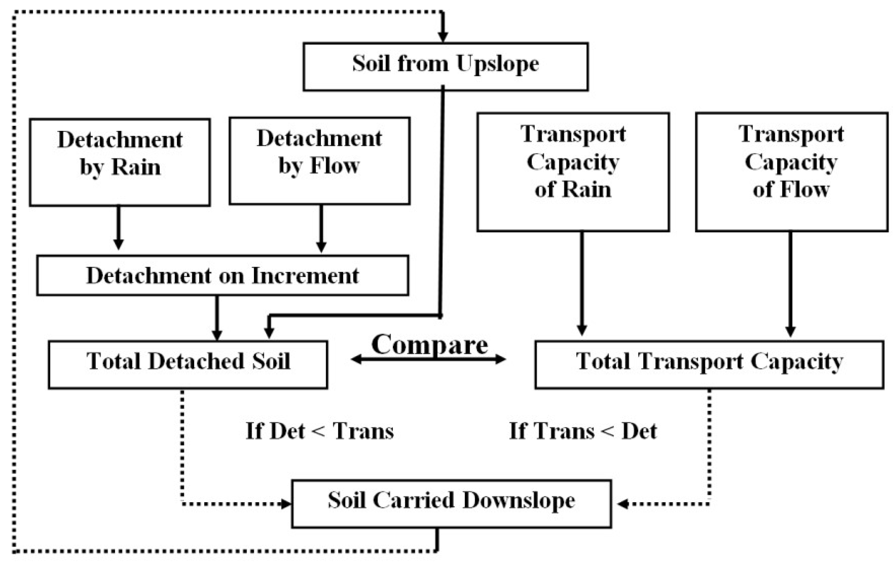
In RUSLE2, the concept of sediment deposition occurring when the sediment transport capacity of the sediment transport system is exceeded by the amount of sediment that is presented to be transported. This approach stems from the scheme developed by Meyer and Wischmeier [50], which is presented in Figure 4. Generally, the transport capacity within a section that is uniform with respect to vegetation and slope gradient is considered to exceed the sediment load generated by erosion, and deposition occurs only when a change in the vegetation or slope gradient causes the transport capacity to fall below the existing sediment load. In RUSLE2, the transport capacity is computed as a function of runoff rate, slope steepness, and hydraulic resistance. RUSLE2 uses the 10-year, 24-h precipitation amount and the NRCS curve number method to compute runoff for this purpose. RUSLE2 takes into account the effects of hydraulic roughness from the soil surface roughness, live ground cover, ground cover provided by crop residue and mulch, and vegetative retardance in determining the transport capacity as it varies along the slope. Once the change in transport capacity causes deposition to occur in a vegetated area, RUSLE2 deposits soil material over a length of slope. If that is shorter than the vegetated area, erosion commences again downslope of the deposition area. The deposition of soil material is dealt with in the same manner when the change in transport capacity is associated with a reduction of slope gradient. As with deposition associated with vegetation, erosion recommences downslope of the deposition zone.

The approach to modeling erosion and deposition adopted in RUSLE2 enhances the capacity of the USLE/RUSLE model to deal with variations in topography and vegetation that occur on one-dimensional hillslopes. The approach can be extended to watersheds [51]. Pandey et al. [52] reviewed 50 soil and sediment yield models, many using the USLE/RUSLE model, to predict erosion, and a variety of different methods have been used to determine the sediment transport capacity. Most of the models developed for agricultural watersheds (catchments) required site-specific calibration before application.

4. Dealing with the Effect of How Soil Loss Varies during the Year

The original objective of the USLE was to determine the long-term average annual soil loss and the simplicity of Equation (1) can lead to the impression that the USLE family of models provides a simple approach to soil loss prediction for management purposes. Equation (1) can also lead to the view that the factors are determined in isolation from each other. In reality, to obtain appropriate values for each factor is not simple, and there are interactions between the factors that have to be taken into account. What was seen as a relatively simple empirical model has, over time, developed more complexity in order to deal with the increasing demands to model the wide variety of agricultural systems that exist today.

As noted above, it has always been recognized that climate and crop systems interact to determine values of the C factor. It is common practice to collect rainfall data on a daily basis over a long period of time such as 20 years, and aggregate it to give average annual values for periods such as a week, a month, or a cropping period. In theory, data on the amount of EI₃₀ and the availability of short-term values of C during the five cropping periods enable soil loss to be predicted during each period in the USLE. This approach was modified in the RUSLE to predict soil loss during 12 half-monthly periods. In RUSLE2, the time step was set to one day, because this provided flexibility in dealing with the time when various activities that influence soil loss occur [8]. In order to do this, daily values of factors such as rainfall amount, EI₃₀, K, C, and P are determined by disaggregating longer-term data. These daily values are used to predict soil loss from bare fallow and cropped areas on a daily basis, so that the total of these daily losses predicts the average annual soil loss. Adding the daily soil loses together for any shorter period provides an estimate of the soil lost during that period. The approach adopted by RUSLE2 can be described by:

$$A_T={\displaystyle \sum _{d=1}^N{R}_d{K}_{d}LS{C}_d{P}_d}$$

(43)

where A_T is the total soil loss (mass per unit area) in a period of time, and N is the number of complete days in that period. Since the daily values are influenced directly by any change that occurs on a day-to-day basis, the model responds directly to temporal variations in the factors that affect soil loss that are associated with crops and crop management. C_d values vary with time depending on canopy cover and configuration, ground cover, surface roughness, ridge height from cultivation, soil biomass, soil consolidation, and soil moisture (https://fargo.nserl.purdue.edu/rusle2_dataweb/userguide/RUSLE2_User_Ref_Guide_2008.pdf).

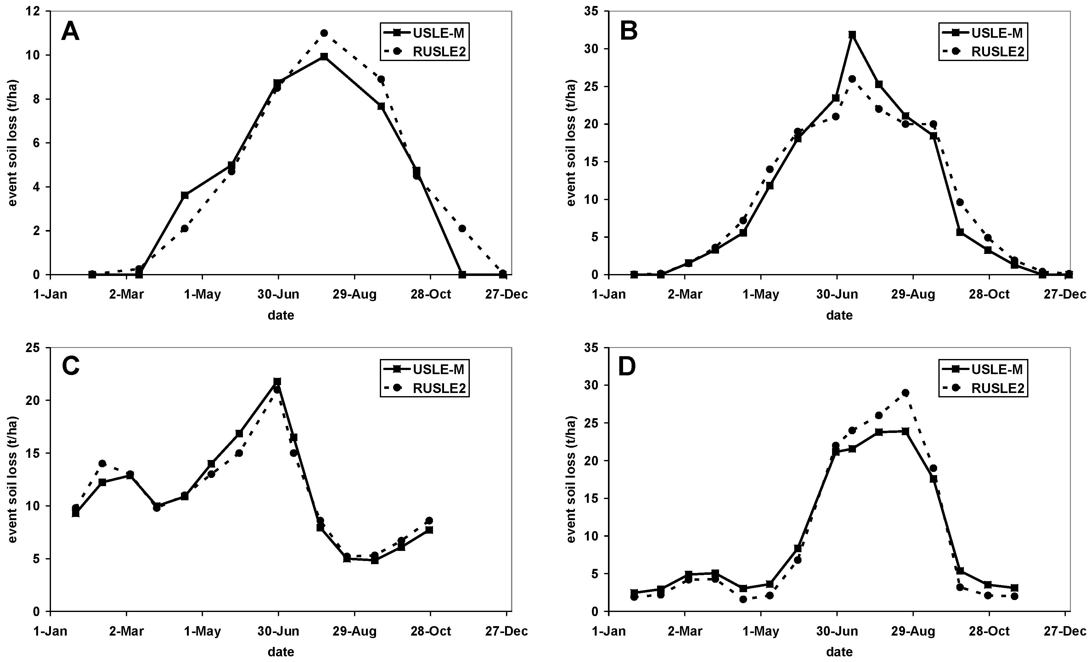
Although the approach used in RUSLE2 was designed to determine soil losses between particular activities undertaken during the year, it also provides the capacity to predict rainfall amount and soil losses for a rainy day as being the sum of the daily soil losses calculated using Equation (43) since the previous rainy day. Consequently, together with prediction of runoff using the curve number method [32], the availability of data on a daily basis facilitates the prediction of runoff and soil loss from bare fallow for a set of design storms at a location [33]. Figure 5 shows the storm soil losses for the design storms predicted by RUSLE2 and the USLE-M at four locations in the USA. The respective storm erodibilities for the RUSLE and USLE-M approaches for the four locations are shown in Figure 3. Multiplying those soil losses by the values of C on the respective days provides an estimate of the soil losses from the cropped area associated with the set of design storms at a location. It should be noted that RUSLE2 predicts within-year average annual soil losses that are the same every year rather than varying between wet and dry years.

RUSLE2 also has the capacity to predict soil losses when users enter EI₃₀ data for specific days. This enables predictions by RUSLE2 to be compared with losses observed for actual events that occurred on runoff and soil loss plots such as those used to develop the USLE. Figure 6 shows the relationships between observed soil losses and losses predicted using the USLE, the USLE-M using observed runoff, RUSLE2 with the user entering EI₃₀ values, and the USLE-M with runoff predicted using RUSLE2 for events observed on plots 1–3 at Presque Isle, ME. The Nash–Sutcliffe efficiency index (NSE) [39] is often used to judge how effective a model is in predicting results. The index has a value of 1.0 for the perfect model, and zero in the model prediction is no better than using the mean. When the Nash–Sutcliffe efficiency index was applied to log transforms of the data (NSE(ln)):

$$NSE\left(ln\right)=1-\frac{{\displaystyle \sum _{n=1}^N{\left(ln{\gamma }_o–ln{\gamma }_m\right)}^2}}{{\displaystyle \sum _{n=1}^N {\left(ln{\gamma }_o–M_{lno}\right)}^2}}$$

(44)

where Y_o is the observed value, Y_m is the modeled value, and M_lno is the mean of the log transforms of Y_o; the USLE-M approach using observed runoff predicted event soil losses the best. RUSLE2 using user-entered EI₃₀ values predicted event soil losses only marginally better than the USLE, and using runoff predicted by RUSLE2 produces a poor prediction of event soil loss when the USLE-M was used.

Table 1. Nash–Sutcliffe efficiency index (NSE(ln)) values obtained soil loss predictions on the four bare fallow plots in the USLE database using the USLE, RUSLE2, and the USLE-M. All the plots were 22.1 m long (source: Kinnell [53]). OH: Ohio, TX: Texas.

					NSE(ln)
Location	Plot No	Gradient %	QR.rope	No of Obs	USLE	RUSLE2	USLE-M with Obs Runoff	USLE-M with RUSLE2 Runoff
Holly Springs, MS	3–7	5.0	0.64	166	0.528	0.563	0.703	0.376
Zanesville, OH	1–8	12.0	0.59	287	0.646	0.644	0.728	0.469
Tyler, TX	1–9	8.8	0.30	192	0.342	0.372	0.696	0.358
Presque Isle, ME	1–3	8.0	0.29	102	0.177	0.190	0.766	−0.442

shows that the results shown for Presque Isle are mirrored at Holly Springs, MS, Zanesville, Ohio (OH), and Tyler, Texas (TX).

As an alternative to RUSLE2, WEPP [4], a more physically-based model of rainfall erosion than RUSLE2, predicts soil loss on an event basis using rainfall events that are generated stochastically over many years by a model called CLIGEN [54]. Given that rainfall is not distributed evenly through time, it can be argued that the event soil losses predicted by WEPP are more realistic than those predicted by RUSLE2. However, the capacity to predict event soil losses for storms that do not occur at regular intervals through user-entered storm data enables CLIGEN to be used as a climate generator for RUSLE2. The relevant CLIGEN climate files can be obtained using WEPP for Windows. CLIGEN does not calculate EI₃₀ values, but these can be obtained using data provided by RUSLE2. RUSLE2 produces a table that contains daily “erosivity densities” during a calendar year at a location. As noted above, erosivity density is the EI₃₀ per unit quantity of rain [8]. The daily erosivity densities used in RUSLE2 are disaggregated from monthly erosivity densities computed for many (>1500) locations in the USA. These monthly erosivity densities were determined as ratios of the monthly sums of EI₃₀ for rains where more than 12.5 mm fell to the monthly amounts of rain obtained from meteorological data that included rains where less than 12.5 mm fell. This approach facilitates the use of generally available meteorological data to predict erosivity rather than less available data for rainstorms where amounts exceed 12.5 mm.

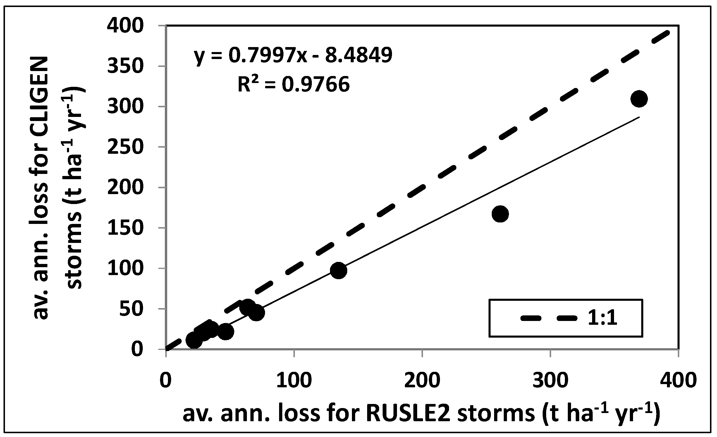
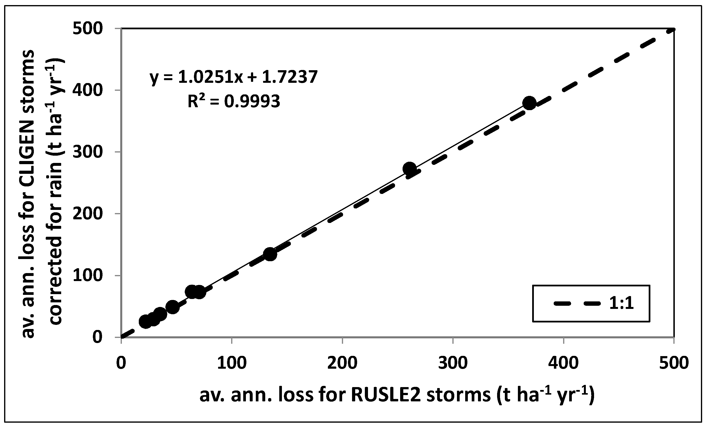
CLIGEN produces many daily rainfalls with low amounts. However, in determining R values for RUSLE2, storms producing less than 12.5 mm of rain were omitted as in RUSLE2. Figure 7 shows the relationship between average annual loss produced by CLIGEN rains >12.5 mm using the RUSLE2 EI₃₀ values over 30 years, and the average annual soil losses predicted by the RUSLE2 representative storms at the six locations listed in

Table 2. RUSLE2 R factor and soils at the locations with unit plots where CLIGEN was used as a weather generator for RUSLE2. IA: Iowa, MI: Michigan, SD: South Dakota, OK: Oklahoma, NY: New York.

Location	State	County	Soil	RRUSLE2
Bethany	MO	Brooke	Selby (sl)	3330
Castana	IA	Monona	Monona (l)	2650
Holly Springs	MI	Marshall	Providence (sil)	6360
Madison	SD	Lake	Egan (sicl)	1330
Presque Isle	ME	Aroostook	Caribou (Gr-l)	1230
Tifton	GA	Tilt	Tifton (sl)	7110
Watkinsville	GA	Oconee	Cecil (scl)	5050
Guthrie	OK	Logan	Stephensville (fsl)	3800
Geneva	NY	Ontario	Ontario (l)	1380

. Although rainfalls of less than 12.5 mm were not included in the calculation of monthly erosivity, as noted above, the amounts of rainfall used to determine daily erosivity density did include rainfalls of less than 12.5 mm, because the daily rainfall amounts were disaggregated from standard meteorological data. Consequently, EI₃₀ values for the CLIGEN storms omitting 12.5-mm rainfalls were underestimated. This can be corrected by multiplying the daily erosivity density values by the ratio between the average annual rainfall recorded in RUSLE2 for the location and the average annual rainfall obtained by CLIGEN when rainfalls less than 12.5 mm were omitted. Figure 8 shows that when this correction is applied, CLIGEN can be used to predict the same average annual soil losses as the RUSLE2-generated storms. In contrast to the RUSLE2-generated storms, the annual soil losses generated using CLIGEN varied between years. CLIGEN version 5.3 was used to generate the data in Figure 8. RUSLE2 erosivity density data may need to be updated when newer versions of CLIGEN that include data on climate change since 2000 are used.

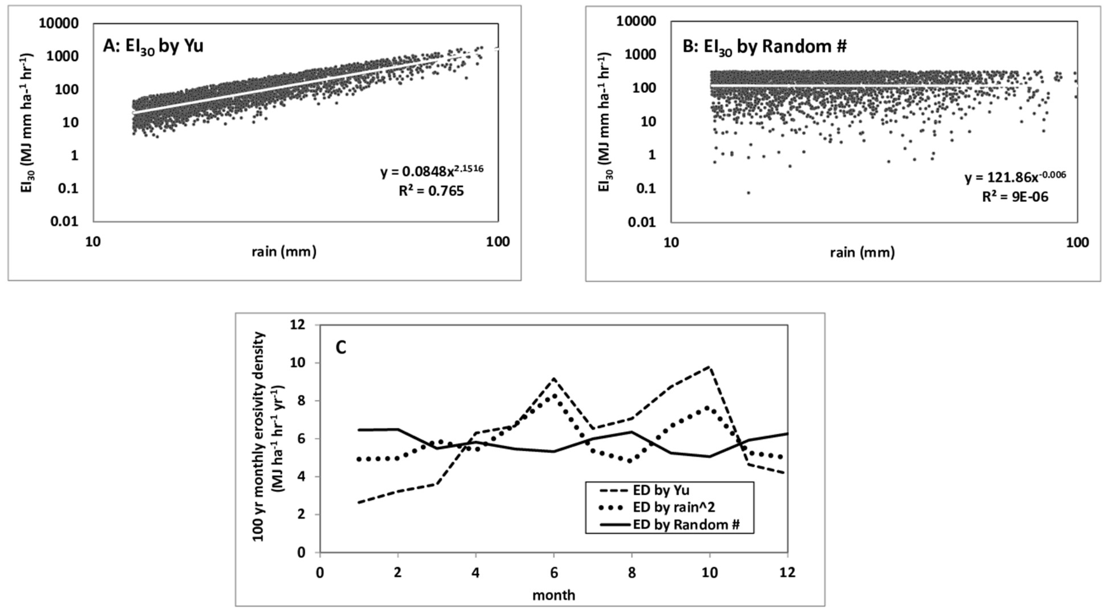
In addition to obtaining EI₃₀ values from the data in RUSLE2, EI₃₀ values for CLIGEN-generated rainfalls can be computed using a method developed by Yu [56]. Yu developed a numerical method that was specifically designed to compute daily EI₃₀ values from daily rainfall-related weather variables generated by CLIGEN. Algorithms were developed to compute the R factor, its monthly distribution, and the 10-year storm EI₃₀ needed to apply the RUSLE. The primary theory used overestimated EI₃₀ values, but an adjustment factor of 0.576 was found to be appropriate throughout the USA. This overestimation could be due to the way that CLIGEN assumes that all the rainfall that falls on a day acts as single event, whereas in the USLE/RUSLE, EI₃₀ values for a day are summations of multiple small events. The method generates adjusted EI₃₀ values for all the CLIGEN-generated rainfalls at a location, and consequently, adjustment is required to model erosion omitting rains of less than 12.5 mm. This can be done by multiplying EI₃₀ values by the ratio of R specified by RUSLE2 for the location and the value of R obtained by CLIGEN when rainfalls of less than 12.5 mm were omitted. In RUSLE2, erosivity densities in the USA tend to show monthly variations that have a triangular profile with a peak in midsummer, but this is not necessarily the case with the erosivity densities obtained using the Yu method (Figure 9). When CLIGEN was applied to predict average annual soil losses from bare fallow and cropped areas using both the Yu method and the RUSLE2 erosivity density method at seven locations in the USA, both methods produced results that were comparable to those produced by RUSLE2 operating in its standard mode (

Table 3. Annual soil loss from plots predicted by RUSLE2 and by using CLIGEN for 100 years with R_d values predicted by the Yu method and RUSLE2 erosivity density values (source: Kinnell and Yu (under review) [57]).

Location	RUSLE2 R	Length	Slope	RUSLE2 K	Treatment	Average Annual Soil Loss
						std RUSLE2	EI30 by Yu	EI30 by R2 ED
	MJ mm/(ha hr yr)	m	%	t hr/(MJ mm)		t/ha/yr	t/ha/yr	t/ha/yr
Bethany	3330	22.3	7.0	0.085	continous bare fallow	201.4	201.6	204.5
					112 bu corn	52.7	52.5	55.8
					NT-corn soybeans NT-wheat	15.6	16.1	15.7
Castana	2650	22.1	14.0	0.030	continous bare fallow	132.2	132.9	134.1
					112 bu corn	34.2	34.4	36.9
					corn soybeans	19.4	19.7	20.6
Geneva	1380	22.1	7.7	0.042	continous bare fallow	39.8	40.5	40.3
					112 bu corn	8.7	9.2	9.1
					Winter Wheat	4.0	4.1	3.8
Guthrie	3800	22.1	8.0	0.011	continous bare fallow	76.4	76.8	76.9
					112 bu corn	26.4	26.8	27.5
					wheat soybeans	5.4	5.5	5.5
Holly Springs	6360	22.1	5.0	0.044	continous bare fallow	206.6	207.4	202.9
					112 bu corn	50.5	50.0	52.2
					cotton (fall chisel)	91.3	91.6	89.3
Madison	1670	22.1	5.6	0.071	continous bare fallow	55.5	54.0	55.3
					112 bu corn	12.9	12.0	12.8
					corn soybeans	6.6	6.4	6.5
Watkinsville	5050	22.1	7.0	0.027	continous bare fallow	103.1	101.4	102.8
					112 bu corn	27.1	26.3	26.8

, Figure 10). The values of R_d generated by using RUSLE2 erosivity densities produce short-term soil losses that are less variable than produced when R_d values are generated by the Yu method (e.g., Figure 11), but those differences have little impact on the prediction of the long-term average annual soil loss (Table 3). CLIGEN version 5.3 was used here, and it should be noted that adjustment to match RUSLE2 R values does not necessarily allow for possible climate change effects that may be incorporated in newer versions of CLIGEN.

Apart from using RUSLE2 erosivity densities and the Yu method, it is possible to predict long-term soil losses using other methods of generating EI₃₀ values from event rainfall amounts. One approach is to predict daily EI₃₀ as a power of daily rainfall [58]:

EI₃₀ = a rain^c

(45)

where a and c are empirical coefficients. For the Yu method, c has a value of about 2.2 at Watkinsville (Figure 12). Using Equation (45) with c = 2.0 produces monthly erosivity densities, as shown in Figure 12C, in comparison with those produced by the Yu method and the assumption that EI₃₀ values are actually completely random. When the four methods of obtaining EI₃₀ values for use with CLIGEN were applied on the bare and cropped soil loss plots at the seven locations in the USA, all the produced predictions were highly correlated with those predicted by RUSLE2 operating in its standard mode. The actual values of soil loss generated on a daily or monthly basis using CLIGEN have no physical meaning, but are generated to produce a set of values that lead to the prediction of the long-term average soil loss, as has been demonstrated by the data presented in Table 3 and

Table 4. Regression analysis for the relationships between average annual soil loss predicted by RUSLE2 operating in its standard mode (A_RUSLE) and average annual soil loss predicted by CLIGEN (A_CLIGEN) when R_d values are generated by different methods at the seven locations.

Model	ARUSLE2 = b ACLIGEN
CLIGEN EI30 by	b	r2	Mean abs Error
Yu method	1.0005	0.9999	0.528
RUSLE2 ED	1.0023	0.9993	1.113
Rain2	1.014	0.9985	1.629
Random number	0.9928	0.9983	2.183

and Figure 10.

5. Accounting for the Effects of Rill Erosion

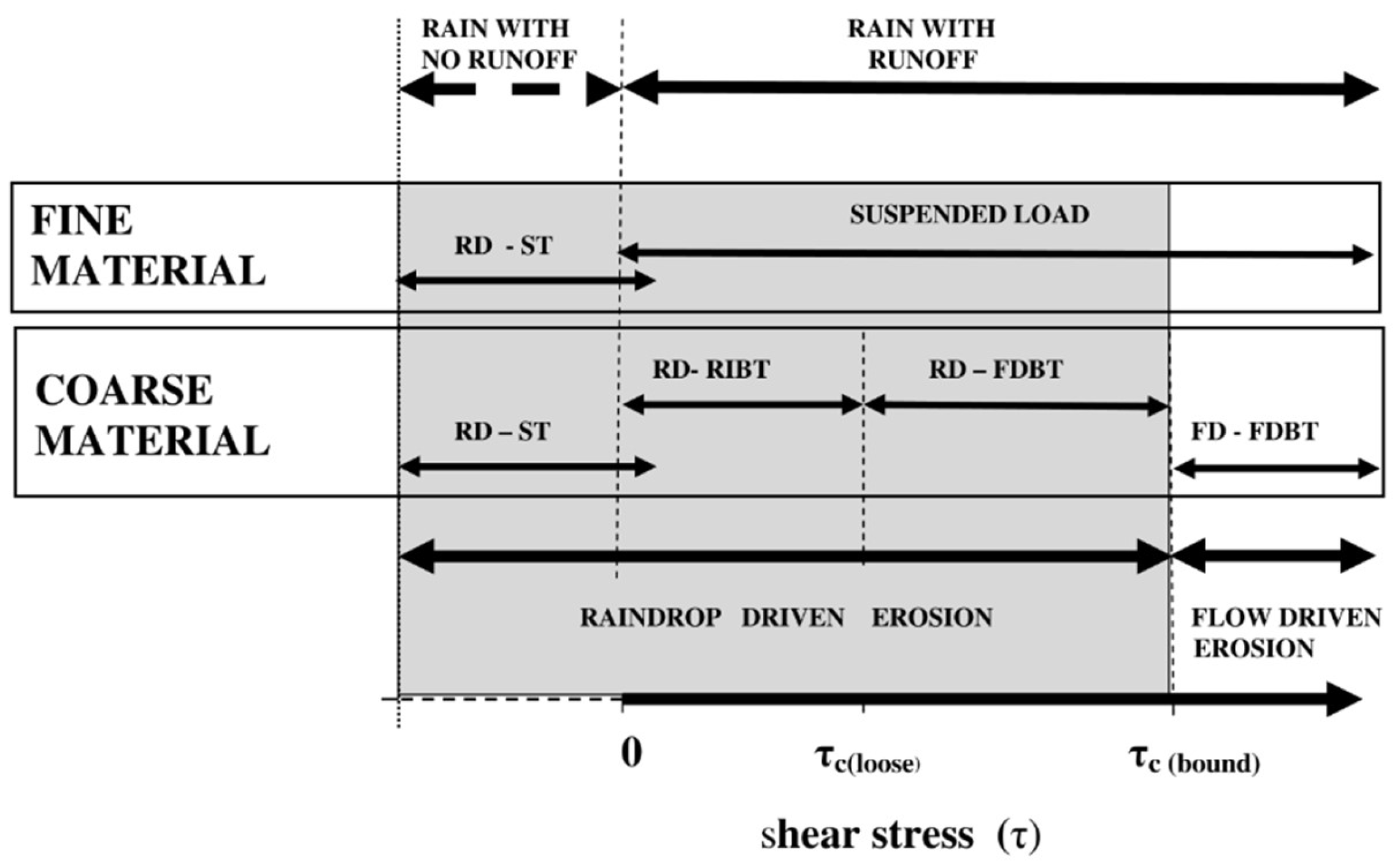
USLE-based models predict soil loss from areas subjected to sheet and rill erosion. In sheet erosion, the area is subjected to raindrop-driven erosion. Raindrop-driven erosion occurs when detachment, the liberation of soil materials from the surface of the soil matric where they are held by cohesion and interparticle friction, results from raindrops impacting the soil surface directly or through a layer of water sitting on the surface. Initially, when rain starts and no water flows over the surface, raindrop-detached material moves over the surface by splash. As time progresses and runoff occurs, there is a transition from transport by splash to transport by rain-impacted flow [59]. Whenever flowing water occurs, fine material is transported by the flow in complete suspension. Above a certain critical shear stress (τ_c(loose), Figure 13), flows have a capacity to transport coarse material by flow-driven bed load transport (FDBT), namely flow-driven saltation and flow-driven rolling. In rain-impacted flows, the coarse material is transported by raindrop-induced bedload transport (RIBT), namely raindrop-induced saltation and raindrop-induced rolling, when the flow shear is below the critical shear stress. With RIBT, coarse material is transported through an interaction between the raindrop impacts and the flowing water. Once the flow acquires a shear stress that exceeds the critical shear stress required for the flow to detach particles held by cohesion and interparticle friction (τ_c(bound)), flow-driven erosion occurs. Once rilling commences, flows that originally moved in a “sheet” down along the surface are encouraged to flow toward the rills. This results in thin flows occurring in the interrill areas where raindrop-driven erosion dominates, while flow-driven erosion takes place in the rills. Detachment and transport within rills results in an increase in the rate soil loss that occurs from that area. In the plot experiments providing the data on which the USLE was based, the surfaces were cultivated between storms to eliminate rills. Conceptually, the erodibility of the soil differs between storms that just cause sheet erosion and storms that produce rill erosion. However, the extent and severity of rilling was not monitored, so a different approach was adopted. As noted earlier, in the RUSLE, the variation in m in the slope length equation (Equation (31)) is dependent on the degree of rilling that occurs on the eroding surface.

In more physically-based models such as WEPP, raindrop-driven erosion and flow-driven erosion are modeled specifically. Foster et al. [24] proposed that using two erosivity indices, one focusing on raindrop-driven erosion and the other focusing on flow-driven erosion, might be useful in accounting for event erosivity (R_e):

R_e = 0.5 EI₃₀ + 0.5α  q_e(q_p)^0.333

(46)

where α is a factor that causes the average annual value of R_e produced by Equation (46) using q_e and q_p values obtained for the unit plot to equal the average annual value of R_e when R_e = EI₃₀. Equation (46) focuses on the situation where the contributions for raindrop-driven erosion and flow-driven erosion are equal. Given that the Q_Re1EI₃₀ index is actually derived from considering soil loss to be directly related to the product of event runoff and event sediment concentration (soil loss per unit runoff), the suggestion that flow-driven erosion is dependent on the product of a power of runoff and a power of peak runoff (Q_p), when combined with Equation (29) could perhaps lead to a useful equation for soil loss from the unit plot being given by:

A_e1 = Q_e1 (a K_UMe ε_e + b K_qe Q_e1^c Q_p^d)

(47)

where Q_e1 is the event runoff from the unit plot, K_UMe is the event erodibility associated with the Q_R1EI₃₀ index, ε_e is the erosivity density (EI₃₀ per unit quantity of rain), K_qe is the event erodibility associated with using the product of Q_e1 and Q_p as an erosivity index for erosion associated with rilling, c and d are empirically derived values, and a and b are coefficients that adjust for the variations in contributions from raindrop-driven and flow-driven erosion [53].

In WEPP, rill and interrill erosion are determined using dedicated soil erodibility factors with a critical shear stress acting as the trigger for rill erosion to occur:

D_f = D_c (1 − G/T_c)

(48)

and:

D_c = K_r (τ_f − τ_c)

(49)

where D_f is the rill erosion rate (mass/area/time), D_c is the detachment capacity of the flow, G is the sediment load, T_c is the sediment load at the transport capacity of the flow, K_r is the rill soil erodibility, τ_f is the shear stress of the flow in the rill, and τ_c is the critical shear stress that needs to be exceeded before detachment in rills occurs. However, even when the erodibility factors and the value of the critical shear stress are calibrated so that WEPP predicts the total soil loss for the set of events involved, it has been shown by Kinnell [53] that the USLE-M predicts event soil losses from bare fallow plots in the USLE database better than WEPP (

Table 5. NSE(ln) values for WEPP and USLE-M for the prediction of observed event soil losses from 22-m long bare fallow plots in the USLE database when runoff for both models was predicted by WEPP. NB: WEPP does not predict soil loss to occur for all the storms where soil loss was observed. Calibration for runoff and soil loss was undertaken using storms where WEPP predicted soil loss did occur, and this ensured that the total runoff and soil loss for both models matched the total runoff and soil losses for the events involved (source: Kinnell (under review) [53]).

			NSE(ln)
Location	Plot No	Gradient %	Runoff	WEPP	USLE-M with WEPP Runoff	Mode
Bethany, MO	1–9	7.0	0.123	−0.394	0.300	validation
			0.153	−0.258	0.317	calibration
Holly Springs, MI	C5	5.0	0.656	0.239	0.538	validation
			0.689	0.375	0.605	calibration
Presque Isle, ME	1–3	8.0	−0.125	−0.440	0.214	validation
			0.156	−0.115	0.296	calibration
Tifton, GA	1–2	3.0	0.319	−1.231	−0.283	validation
						calibration
Watkinsville, GA	2–47	7.0	0.281	−0.888	0.280	validation
			0.320	−0.797	0.362	calibration

). Even though an empirical model based on the conceptual approach presented in Equation (47) could initially appear useful in modeling erosion using USLE-based modeling systems, the modeling of temporal variations in rilling successfully through coefficients a and b may be extremely difficult to acheive. Increasing model complexity can lead to increased model uncertainty ([60,61]).

6. The Unit Plot as the Physical Model

As noted above, conceptually, the unit plot provides the physical model on which the USLE is based. In most of the locations where the bare fallow plots were installed in the USA, a unit plot did not exist. Certainly, slope lengths of 22.1 m were common, but as indicated in Table 5, slope gradients were usually different from 9%. In some cases, bare fallow plots of 22.1 m were also not installed. Consequently, in order to determine the K values for those locations, the observed soil loss values were adjusted to estimate the losses from the unit plot situation using the S and L factor equations. Also, as noted above, the unit plot provides the situation where spatial variations in R and K can be determined independently of all the effects that topography and vegetation have on soil loss. As such, using the unit plot approach can be perceived as providing a sound foundation to the modeling of rainfall erosion.

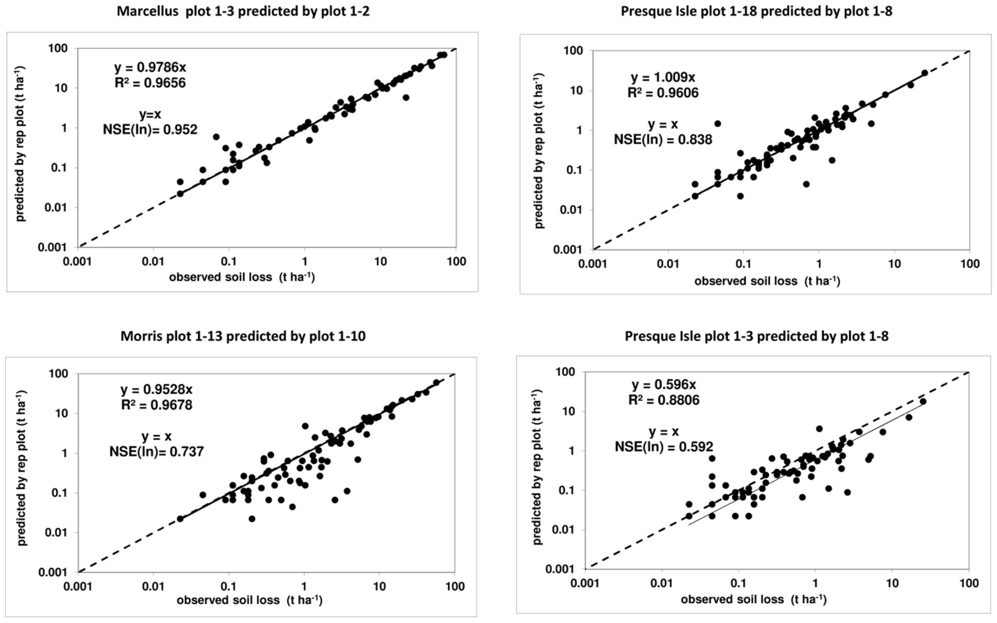
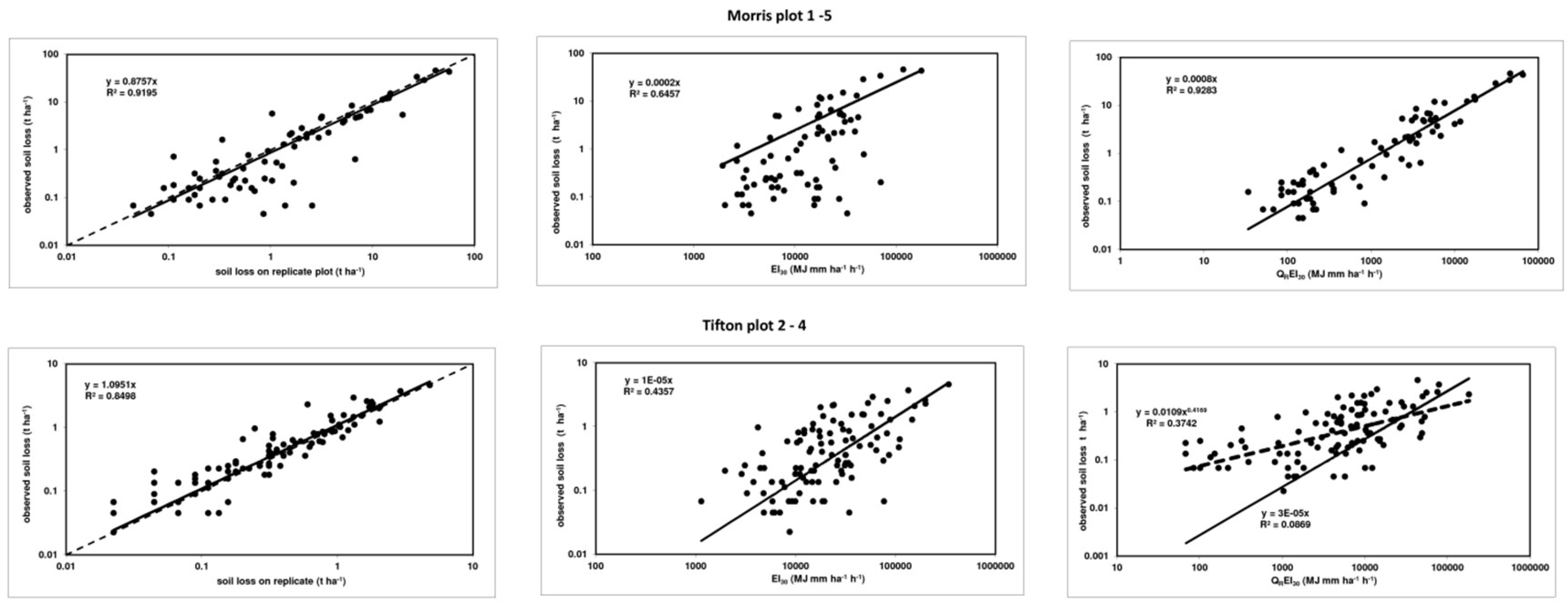
It has been proposed that the best physical model of erosion from a plot is provided by a replicate plot [62]. Replicates of bare fallow plots were installed at a number of locations in the USA, and Figure 14 shows the predictions of observed event soil losses from observed soil losses from a replicate at three locations. For 23 plots at 11 locations in the USA, NSE(ln) values ranged from 0.592 to 0.957 (

Table 6. NSE(ln) values when USLE, USLE-M, and replicate models were applied to bare fallow plots in the USLE database (source: Kinnell [63]).

				NSLE(ln)
Location	Obs	Principal	Replicate	REPLICATE	USLE	USLE-M
Presque Isle	82	plot 1–3	plot 1–8	0.592	0.091	0.693
Presque Isle	85	plot 1–8	plot 1–18	0.838	0.137	0.772
Marcellus	65	plot 1–2	plot 1–3	0.957	0.365	0.786
Marcellus	65	plot 1–3	plot 1–2	0.952	0.366	0.771
Morris	74	plot 1–5	plot 1–10	0.706	0.015	0.838
Morris	74	plot 1–10	plot 1–13	0.636	0.133	0.784
Morris	74	plot 1–13	plot 1–5	0.737	−0.078	0.758
Castana	116	Plot 1–3	plot 1–4	0.829	0.396	0.777
Castana	116	plot 1–4	plot 1–3	0.878	0.307	0.809
Bethnay	135	plot 1–9	plot 1–10	0.772	0.498	0.761
Bethnay	135	plot 1–10	plot 1–9	0.765	0.396	0.716
McCredie	124	plot 2–1	plot 2–18	0.763	0.332	0.842
McCredie	124	plot 2–18	plot 2–1	0.742	0.058	0.548
LaCrosse	97	plot 1–8	plot 1–9	0.828	0.566	0.854
LaCrosse	97	plot 1–9	plot 1–8	0.832	0.547	0.853
Holly Springs	187	plot 3–5	plot 3–7	0.826	0.520	0.645
Holly Springs	187	plot 3–7	plot 3–5	0.843	0.491	0.704
Watkinsville	111	plot 2–47	plot 2–64	0.722	0.443	0.594
Watkinsville	111	plot 2–64	plot 2–47	0.765	0.354	0.453
Madison	66	plot 1–5	plot 1–12	0.893	0.024	0.781
Madison	66	plot 1–12	plot 1–5	0.886	0.058	0.751
Tifton	103	plot 1–2	plot 2–4	0.820	0.263	−0.511
Tifton	103	plot 2–4	plot 1–2	0.838	0.157	−0.346

). The NSE(ln) values shown in Table 6 were determined by the variation from the 1-to-1 dotted line shown in Figure 14. These differences result from both the stochastic and systematic differences between the observed and predicted values. Also shown in Figure 14 are data for regressions between the observed and predicted values. Values of the regression coefficients close to 1.0 indicate that the effect of systematic differences is minimal. In the case of the data presented in Table 6, the effect on NSE(ln) values when systematic differences dominate is indicted by the dotted lines in Figure 15. Low values of NSE(ln) when the regression coefficient is close to 1.0 indicate situations where stochastic differences dominate. In addition to the NSE(ln) values for the observed—i.e., replicate—model, values of NSE(ln) for the USLE and USLE-M using observed runoff are presented in Table 6, in which the erodibility values were determined individually for the plots being considered. In many cases, the USLE-M performed at a comparable level to the replicate model. Some improvement in the NSE(ln) values could result from using Equation (23), particularly at Tifton, GA, where b1 = 0.419 (Figure 16). However, even when the model used may show systematic errors, because the soil erodibility factor is determined as the total soil loss for a number of events divided by the total value of the erosivity index for those storms, the model focuses on predicting the total soil loss well irrespective of the erosivity index used or whether the relationship between the index and soil loss is linear or non-linear.

In examining the ability of replicates to predict event soil loss from the primary plot, only storms where both plots produced erosion were used, even though there were, at times, soil losses measured on replicates when none was measured on the principal plot. In using the unit plot approach, it is assumed that if soil loss occurs on the unit plot, it will also occur in the area of interest. Obviously, that assumption does not necessarily hold true when considering soil losses on a storm-by-storm basis on bare fallow plots, and consequently, the K values determined for replicated plots are usually for each individual plot.

Although a replicate plot may be considered to provide the best physical model of erosion from a plot, variations in the values of K occur within a set of replicates. The experimental study by Wendt et al. [64] is often cited to illustrate the variability between replicates. In the experiment, 40 bare plots were cultivated, and in other ways treated identically. Wendt et al. observed that the spatial variations in the total runoff and soil loss produced by 25 storms in 1981 were not readily related to measured plot properties. They also concluded that the importance of plot differences did not persist in runoff and soil loss data obtained before or after the 25 events. However, that conclusion was based on data from a six-year experiment with seven conventional and six no-till corn plots prior to 1981, and three storms on runoff and soil loss plots for fallow together with corn and soybeans using three tillage methods in 1983, so that the comparison is hardly robust. For individual storms, Wendt et al. observed coefficients of variation varying from 18% to 91%, in which the highest relative differences were associated with small events. Wendt et al. did acknowledge that a portion of the variability between plots that they observed could have been the result of spatial variations in erodibility. They noted that tillage may have contributed to different microtopographies, but no quantitative evaluations of flow patterns were made. Gomez et al. [65] also concluded that changes in the relative difference in runoff between the plots used by Wendt et al. might be explained by modifications of the spatial distribution of the saturated hydraulic conductivity and surface storage during cultivation. As a general rule, replicates act as good physical models of plots when soil losses are high [62].

As noted above, in developing the USLE, the unit plot was specified as being a bare fallow area that was 22.1-m long on a 9% slope where cultivation was done up and down the slope. It was also noted that the lack of plots meeting this specification resulted in K being determined from non-unit plots by using the L and S factors to adjust the observed soil losses to those expected to occur on unit plots if they had existed. There are situations where the K factor values so calculated are appreciably different from those that would have been obtained had the unit plots existed, because the rilling situation on the unit plot would have been appreciably different than that on the non-unit plot. Given that high slope gradients are used in China, the Chinese version of the USLE specifies the unit plot to be a bare fallow 20-m long on a 15-degree (26.8%) slope with cultivation done up and down the slope [66]. Plots meeting this specification exist in China.

There is an expectation that the two-step mathematical approach used in the USLE applies in modeling event erosion from cropped areas so that:

A_eC = A_e1 K_e L S C_e P_e

(50)

where A_eC is the soil loss for an event on a cropped area. However, the two-step mathematical approach does not necessarily work well with vegetative areas, because runoff may not necessarily occur on both bare and cropped surfaces during a storm. Consequently, as indicated by Figure 17A, the two-step model predicts event soil losses to occur on cropped areas when they do not. As an alternative, the Q_REI₃₀ index approach provides the means to predict event soil loss from vegetated areas by using the runoff ratio for a cropped plot (Q_RC) rather than the runoff ratio for the unit plot (Q_R1):

A_eC = Q_ReC EI₃₀ K_e,UM L S C_e.UM P_e.UM

(51)

where K_e,UM, C_e.UM, and P_e.UM are the event values for soil erodibility, crop and crop management, and soil conservation protection when Q_ReCEI₃₀ is used as the event erosivity index. Procedures do not currently exist to estimate K_e,UM, C_e.UM, and P_e.UM, but they do exist to determine the long-term average annual values of K_UM, C_UM, and P_UM [30]. Figure 17B shows the relationship between the observed and predicted event soil losses for the same plot with corn at Clarinda, Iowa (IA) as used in Figure 17A when soil losses were predicted using:

A_eC = Q_ReC EI₃₀ K_UM L S C_UM P_UM

(52)

Unlike the USLE/RUSLE approach, Equation (52) does not operate mathematically in two steps, despite K_UM and K both being determined for unit plot conditions. Consequently, the USLE-M approach adopted in Equation (52) outperforms the two-step mathematical approach used by the USLE/RUSLE model when the runoff from the cropped area is known [53].

7. What Next?

The USLE originated as an empirical model based on more than 10,000 plot years of data obtained in the USA during the middle of the 20th century. The unit plot concept was central to the establishment of the mathematical model in that it provided a base condition in which only R and K were involved in the prediction of soil loss. There is little evidence that an actual bare fallow “unit plot” 72.6 feet (22.1 m) long on a 9% slope with cultivation up and down the slope ever existed [67]. The “unit plot” exists as a reference condition. It could have been longer or shorter, on a steeper or less steep slope. The specification of how K is determined from unit plot data (Equation (9)) is central to the ability of the unit plot approach to predict long-term soil loss from bare fallow areas. It ensures that the total of the product of EI₃₀ and K for a set of runoff-producing storms is equal to the total observed soil loss for that set of storms even when, as shown in Figure 2A, a direct relationship between event soil loss and EI₃₀ does not exist. Using the Q_REI₃₀ index in place of EI₃₀ when event runoff is known reduces systematic errors associated with assuming that a direct relationship exists between event soil loss and EI₃₀ at many locations when runoff is known or predicted well. It has always been known that runoff influences soil loss, but event runoff is difficult to predict well. Including runoff as independent variable in a prediction event of soil loss is an impediment to predicting event soil loss well when runoff is not measured. Awareness of this was one of the reasons why runoff was not considered directly as a factor in determining erosivity in the USLE [68]. This is true irrespective of whether the model is empirically based, such as the USLE-M, or physically based, such as WEPP.

The Revised USLE (RUSLE) maintained the unit plot approach, but changed the way some of the other factors were determined. In including conceptual-based approaches to the determination of factors such as C, RUSLE moved USLE technology from an empirical model to a hybrid one. There has always been a time element involved in the determination of C. RUSLE2 moved the time base from half-monthly to daily in order to deal with the effects of short-term issues that influence soil loss better. Other enhancements included in RUSLE2 were designed to accommodate the specific needs of conservation planners to deal with situations not included in the original USLE database [69]. RUSLE2 is associated with an extensive database in the USA, but has been used in countries such as China [70], Spain [71], Nigeria [72], and Iran [73].

At the end of 2016, notice was give of the intention of the Natural Resources Conservation Service (NRCS) in the USA to implement the WEPP technology to replace the use of the Revised Universal Soil Loss Equation, Version 2 (RUSLE2), where applicable (https://www.federalregister.gov/documents/2016/11/17/2016-27633/notice-of-implementation-of-the-water-erosion-prediction-project-wepp-technology-for-soil). The development of WEPP began in the 1980s, and was driven by the shortcomings of the USLE that limited its applicability to many problems [67]. According to Laflen and Flanagann [67], “It did a very poor job in estimating short-term soil erosion”, and “It did not consider deposition.” The rainfall factor in the USLE expressed detachment as a function of rainfall energy, which is a major weakness when erosion was due to snowmelt or irrigation. The first prototype of WEPP was made public in 1989 and in 1995, the complete and validated version was documented [4] and released. Some of the criticisms of the USLE have been redressed over time in RUSLE2 and the USLE-M. Table 5 shows that the USLE-M predicts event soil losses from runoff and soil loss plots better than WEPP when both models use runoff predicted by WEPP and both models were calibrated to predict the total soil loss for the erosion events involved. RUSLE2 does model deposition resulting from spatial variations in slope gradient and vegetation. The USLE-M is a transport-limited model, and consequently does not need an overriding sediment transport model to deal with deposition. In WEPP, event rainfall timing and amounts are generated stochastically by CLIGEN. RUSLE2 has a capacity to use CLIGEN as a rainfall generator [55]. In addition, the data requirements for so-called physically-based models such as WEPP are immense, and the increase in model complexity tends to increase the uncertainty in the predicted outcomes [74]. In a recent comparison between WEPP and RUSLE2, Srivastava (2017, https://www.slideshare.net/SWCSevents/wepp-model-enhancements-for-nrcs-use) showed that for various cropping systems on various soils at 21 locations in the USA, WEPP predicted on average less average annual soil loss than RUSLE2, and there were often large differences between the predictions by the two models for each crop-location situation. For example, when RUSLE2 predicted an average annual loss of about 36 t ha⁻¹ for a current practice at a location, WEPP predicted about 12.5 t ha⁻¹. When RUSLE2 predicted an average annual loss of 15 t ha⁻¹, WEPP predicted 26 t ha⁻¹. No data on which model actually provided the best prediction of actual average annual soil losses were provided.

With WEPP replacing the use of RUSLE2 by NRCS, RUSLE2 will become a standalone model in the USA, and any further development of USLE-based technology is unlikely to be a priority of the USDA Agricultural Research Service in the future. When WEPP is calibrated to predict observed soil losses, predictions are more sensitive to the calibration of rill soil erodibility and the critical shear stress for rilling to occur than the calibration of interrill soil erodibility [75]. WEPP has a default rill spacing of 1 m. The field rainfall experiments that were undertaken to determine the interill erodibilities for WEPP [76] were done on plots that focused on ridge tillage cultivated areas where that rill spacing is most appropriate. The interrill erodibilities so determined were found not to be appropriate when flat plots were used [77]. Flat plots were commonly used in producing the data used to develop the USLE. Wendt et al. [64] noted that there was not real evidence of rilling in the 40 plots they studied. The ability of WEPP to predict event erosion on the USA runoff and soil loss plots is open to question when USLE based models such as the USLE-M can do the job better, even when WEPP has been calibrated (Table 5).

Soil prediction models such as the USLE and WEPP have three primary uses in agriculture: (a) to assist land managers to choose cropping systems and practices that conserve soil, (b) to make broad-scale surveys to identify the scope of the erosion problem over an area and track changes in erosion over time, and (c) regulate activities for the purpose of conservation compliance [74]. USLE-based technology has been used in all three roles for a long time in the USA, and assists land managers with choosing cropping systems and practices that conserve soil and making broad-scale surveys to identify the scope of the erosion problem over an area and track changes in erosion over time elsewhere. While, for these purposes, there is not great need to predict exactly what soil loss will occur in short term, the ability to predict short-term soil losses well is often seen as something that instills confidence in the results obtained in the longer term. Rainfall erosion is a complex process, but increasing the complexity of models in order to produce better short-term predictions may, as noted by Nearing and Hairsine [61], lead to more uncertainty in the predicted outcomes. Although WEPP may take the lead role in soil loss prediction the USA, USLE-based modeling of erosion is likely to continue outside the USA.

References

1. Wischmeier, W.; Smith, D. Rainfall-erosion losses from cropland east of the Rocky Mountains, guide for selection of practices for soil and water conservation. In Agriculture Handbook; United States Department of Agriculture: Washington, DC, USA, 1965; p. 282. [Google Scholar]
2. Wischmeier, W.H.; Smith, D.D. Predicting rainfall erosion losses—A guide to conservation planning. In USDA Agricultural Handbook; United States Department of Agriculture: Washington, DC, USA, 1978; p. 537. [Google Scholar]
3. Renard, K.G.; Foster, G.R.; Weesies, G.A.; McCool, D.K.; Yoder, D.C. Predicting soil erosion by water: A guide to conservation planning with the revised universal soil loss equation (RUSLE). In U.S. Department of Agriculture Agricultural Handbook. No. 703; US Department of Agriculture: Washington, DC, USA, 1997. [Google Scholar]
4. Flanagan, D.; Nearing, M. USDA-Water Erosion Prediction Project: Hillslope Profile and Watershed Model Documentation; NSERL Report; Flanagan, D., Nearing, M., Eds.; United States Department of Agriculture: Washington, DC, USA, 1995.
5. Zingg, A.W. Degree and length of land slope as it affects soil loss in run-off. Agric. Eng. 1940, 21, 59–64. [Google Scholar]
6. Wischmeier, W.H.; Smith, D.D. Rainfall energy and its relationship to soil loss. Trans. Am. Geophys. Union 1958, 39, 285–291. [Google Scholar] [CrossRef]
7. Laws, J.O.; Parsons, D.A. The relation of raindrop-size to intensity. Trans. Am. Geophys. Union 1943, 24, 452–460. [Google Scholar] [CrossRef]
8. USDA, Draft User’s Reference Guide Revised Universal Soil Loss Equation Veraion 2; USDA-Agricultural Research Service: Washington, DC, USA, 2008.
9. Nearing, M.A.; Yin, S.Q.; Borrelli, P.; Polyakov, V.O. Rainfall erosivity: An historical review. Catena 2017, 157, 357–362. [Google Scholar] [CrossRef]
10. Kinnell, P. The Problem of Assessing the Erosive Power of Rainfall from Meteorological Observations 1. Soil Sci. Soc. Am. J. 1973, 37, 617–621. [Google Scholar] [CrossRef]
11. Yang, X.; Yu, B. Modelling and mapping rainfall esosivity in New South Wales Australia. Soil Res. 2015, 53, 178–189. [Google Scholar] [CrossRef]
12. Panagos, P.; Borrelli, P.; Meusburger, K.; Yu, B.; Klik, A.; Lim, K.J.; Yang, J.E.; Ni, J.; Miao, C.; Chattopadhyay, N.; et al. Global rainfall erosivity assessment based on high-temporal resolution rainfall records. Sci. Rep. 2017, 7, 4175. [Google Scholar] [CrossRef]
13. Wischmeier, W.H.; Mannering, J. Relation of soil properties to its erodibility. Soil Sci. Soc. Am. J. 1969, 33, 131–137. [Google Scholar] [CrossRef]
14. Wischmeier, W.H.; Johnson, V.; Cross, C. Soil erodibility nomograph for farmland and construction sites. Soil Water Conserv. J. 1971, 5, 189–193. [Google Scholar]
15. Auerswald, K.; Fiener, P.; Martin, W.; Elhaus, D. Use and misuse of the K factor equation in soil erosion modeling: An alternative equation for determining USLE nomograph soil erodibility values. Catena 2014, 118, 220–225. [Google Scholar] [CrossRef]
16. Dabney, S.M.; Wilson, G.V.; McGregor, K.C.; Foster, G.R. History, residue, and tillage effects on erosion of loessial soil. Trans. ASAE 2004, 47, 767. [Google Scholar] [CrossRef]
17. Romkens, M. The soil erodibility factor: A perspective. In Soil Erosion and Conservation; El-Swaify, S.A., Moldenhauer, W.C., Eds.; Soil and Water Conservation Society of America: Ankeny, IA, USA, 1985; pp. 445–461. [Google Scholar]
18. Kinnell, P.I.A. Accounting for the influence of runoff on event soil erodibilities associated with the EI30 index in RUSLE2. Hydrol. Process. 2015, 29, 1397–1405. [Google Scholar] [CrossRef]
19. El-Swaify, S.A.; Dangler, E.W. Erodibilities of selected tropical soils in relation to structural and hydrologic parameters. In Soil Erosion: Prediction and Control; Soil and Water Conservation Society of America: Ankeny, IA, USA, 1977; pp. 105–114. [Google Scholar]
20. Loch, R.; Slater, B.; Devoil, C. Soil erodibility (Km) values for some Australian soils. Soil Res. 1998, 36, 1045–1056. [Google Scholar] [CrossRef]
21. Bagarello, V.; Di Stefano, C.; Ferro, V.; Giordano, G.; Iovino, M.; Pampalone, V. Estimating the USLE soil erodibility factor in Sicily, south Italy. Appl. Eng. Agric. 2012, 28, 199–206. [Google Scholar] [CrossRef]
22. Panagos, P.; Meusburger, K.; Ballabio, C.; Borrelli, P.; Alewell, C. Soil erodibility in Europe: A high-resolution dataset based on LUCAS. Sci. Total Environ. 2014, 479, 189–200. [Google Scholar] [CrossRef]
23. Tiwari, A.; Risse, L.; Nearing, M. Evaluation of WEPP and its comparison with USLE and RUSLE. Trans. ASAE 2000, 43, 1129. [Google Scholar] [CrossRef]
24. Foster, G.; Meyer, L.; Onstad, C. A runoff erosivity factor and variable slope length exponents for soil loss estimates. Trans. ASAE 1977, 20, 683–687. [Google Scholar] [CrossRef]
25. Williams, J.R. Sediment-yield prediction with universal equation using runoff energy factor. In Present and Prospective Technology for Predicting Sediment Yield and Sources; Volume ARS-S-40; Agricultural Research Service: New Orleans, LA, USA, 1975; pp. 244–252. [Google Scholar]
26. Onstad, C.; Foster, G. Erosion modeling on a watershed. Trans. ASAE 1975, 18, 288–292. [Google Scholar] [CrossRef]
27. Williams, J.W.; Izaurralde, R.C.; Steglich, E. Agricultural Policy/Environmental Extender Model Theoretical Documantation; Blackland Research and Extension Center: Temple, TX, USA, 2008.
28. Williams, J.; Jones, C.; Dyke, P. The EPIC Model. In An Erosion/Productivity Impact Calculator: Model Documentation; Sharply, A.N., Williams, J.R., Eds.; USDA Tech Bulletin; USDA: Washington, DC, USA, 1990. [Google Scholar]
29. Kinnell, P.I.A.; McGregor, K.C.; Rosewell, C.J. The IXEA Index as an Alternative to the El30 Erosivity Index. Trans. ASAE 1994, 37, 1449–1456. [Google Scholar] [CrossRef]
30. Kinnell, P.I.A.; Risse, L.M. USLE-M: empirical modeling rainfall erosion through runoff and sediment concentration. Soil Sci. Soc. Am. J. 1998, 62, 1667–1672. [Google Scholar] [CrossRef]
31. Kinnell, P.I.A. Event soil loss, runoff and the Universal Soil Loss Equation family of models: A review. J. Hydrol. 2010, 385, 384–397. [Google Scholar] [CrossRef]
32. Hawkins, R.H.; Ward, T.J.; Woodward, D.E.; Van Mullem, J.A. (Eds.) Curve Number Hydrology: State of the Practice; American Society of Civil Engineers: Reston, VI, USA, 2008.
33. Dabney, S.M.; Yoder, D.C.; Vieira, D.A.; Bingner, R.L. Enhancing RUSLE to include runoff-driven phenomena. Hydrol. Process. 2011, 25, 1373–1390. [Google Scholar] [CrossRef]
34. Bagarello, V.; Di Piazza, G.V.; Ferro, V.; Giordano, G. Predicting unit plot soil loss in Sicily, south Italy. Hydrol. Process. 2008, 22, 586–595. [Google Scholar] [CrossRef]
35. Bagarello, V.; Ferro, V.; Giordano, G. Testing alternative erosivity indices to predict event soil loss from bare plots in Southern Italy. Hydrol. Process. 2010, 24, 789–797. [Google Scholar] [CrossRef]
36. Bagarello, V.; Ferro, V.; Giordano, G.; Mannocchi, F.; Todisco, F.; Vergni, L. Predicting event soil loss from bare plots at two Italian sites. Catena 2013, 109, 96–102. [Google Scholar] [CrossRef]
37. Kinnell, P.I.A. Determining soil erodibilities for the USLE-MM rainfall erosion model. Catena 2018, 163, 424–426. [Google Scholar] [CrossRef]
38. Bagarello, V.; Di Stefano, C.; Ferro, V.; Pampalone, V. Comparing theoretically suppored rainfall-runoff erosivity factors at Sparacia (Southern Italy) experimental site. Hydrol. Process. 2018, 32, 507–515. [Google Scholar] [CrossRef]
39. Nash, J.E.; Sutcliffe, J.V. River flow forecasting through conceptual models part I—A discussion of principles. J. Hydrol. 1970, 10, 282–290. [Google Scholar] [CrossRef]
40. Di Stefano, C.; Ferro, V.; Pampalone, V. Applying the USLE family of models at the Sparacia (south Italy) experimental site. Land Degrad. Dev. 2017, 28, 994–1004. [Google Scholar] [CrossRef]
41. Moore, I.D.; Burch, G.J. Physical basis of the length-slope factor in the Universal Soil Loss Equation. Soil Sci. Soc. Am. J. 1986, 50, 1294–1298. [Google Scholar] [CrossRef]
42. Foster, G.; Wischmeier, W. Evaluating irregular slopes for soil loss prediction. Trans. ASAE 1974, 17, 305–309. [Google Scholar] [CrossRef]
43. Desmet, P.; Govers, G. A GIS procedure for automatically calculating the USLE LS factor on topographically complex landscape units. J. Soil Water Conserv. 1996, 51, 427–433. [Google Scholar]
44. Yu, B.; Rosewell, C. Evaluation of WEPP for runoff and soil loss prediction at Gunnedah, NSW, Australia. Soil Res. 2001, 39, 1131–1145. [Google Scholar] [CrossRef]
45. Moore, I.D.; Wilson, J.P. Length-slope factors for the Revised Universal Soil Loss Equation: Simplified method of estimation. J. Soil Water Conserv. 1992, 47, 423–428. [Google Scholar]
46. Mutchler, C.; Murphree, C.; McGregor, K. Subfactor method for computing C factors for continuous cotton. Trans. ASAE 1982, 25, 327–332. [Google Scholar] [CrossRef]
47. Borrelli, P.; Meusburger, K.; Ballabio, C.; Panagos, P.; Alewell, C. Object-oriented soil erosion modelling: A possible paradigm shift from potential to actual risk assessments in agricultural environments. Land Degrad. Dev. 2018, 29, 1270–1281. [Google Scholar] [CrossRef]
48. Foster, G.R.; Lane, L.J.; Nowlin, J.D.; Laflen, J.M.; Young, R.A. Estimating erosion and sediment yield on field-sized areas. Trans. ASAE 1981, 24, 1253–1262. [Google Scholar] [CrossRef]
49. Walling, D.E. The sediment delivery problem. J. Hydrol. 1983, 65, 209–237. [Google Scholar] [CrossRef]
50. Meyer, L.; Wischmeier, W. Mathematical simulation of the process of soil erosion by water. Trans. ASAE 1969, 12, 754–758. [Google Scholar]
51. Dabney, S.; Yoder, D.; Vieira, D. The application of the Revised Universal Soil Loss Equation, Version 2, to evaluate the impacts of alternative climate change scenarios on runoff and sediment yield. J. Soil Water Conserv. 2012, 67, 343–353. [Google Scholar] [CrossRef] [Green Version]
52. Pandey, A.; Himanshu, S.K.; Mishra, S.K.; Singh, V.P. Physically based soil erosion and sediment yield models revisited. Catena 2016, 147, 595–620. [Google Scholar] [CrossRef]
53. Kinnell, P.I.A. A comparison of the abilities of the USLE-M, RUSLE2 and WEPP to model event erosion from bare fallow areas. Sci. Total Environ. 2017, 596, 32–42. [Google Scholar] [CrossRef] [PubMed]
54. Nicks, A.; Lane, L.; Gander, G. Weather generator, Chapter 2. USDA-Water Erosion Prediction Project Hillslope Profile and Watershed Model Documentation. NSERL Rep. 1995, 10, 1–123. [Google Scholar]
55. Kinnell, P.I.A. CLIGEN as a weather generator for RUSLE2. Catena 2019, 172, 877–880. [Google Scholar] [CrossRef]
56. Yu, B. Using CLIGEN to generate RUSLE climate inputs. Trans. ASAE 2002, 45, 993. [Google Scholar]
57. Kinnell, P.I.A.; Yu, B. CLIGEN as a weather generator for predicting rainfall erosion using USLE based modelling systems. Land Degred. Dev. 2018. in review. [Google Scholar]
58. Richardson, C.; Foster, G.; Wright, D. Estimation of erosion index from daily rainfall amount. Trans. ASAE 1983, 26, 153–156. [Google Scholar] [CrossRef]
59. Moss, A.; Green, P. Movement of solids in air and water by raindrop impact. Effects of drop-size and water-depth variations. Soil Res. 1983, 21, 257–269. [Google Scholar] [CrossRef]
60. Brazier, R.E.; Beven, K.J.; Freer, J.; Rowan, J.S. Equifinality and uncertainty in physically based soil erosion models: Application of the GLUE methodology to WEPP—The Water Erosion Prediction Project—For sites in the UK and USA. Earth Surface Process. Landf. 2000, 25, 825–845. [Google Scholar] [CrossRef]
61. Nearing, M.; Hairsine, P. The future of soil erosion modelling. In Handbook of Erosion Modelling; John and Wiley and Sons: Hoboken, NJ, USA, 2011; pp. 387–397. [Google Scholar]
62. Nearing, M.A.; Govers, G.; Norton, L.D. Variability in soil erosion data from replicated plots. Soil Sci. Soc. Am. J. 1999, 63, 1829–1835. [Google Scholar] [CrossRef]
63. Kinnell, P.I.A. Comparison between the USLE, the USLE-M and replicate plots to model rainfall erosion on bare fallow areas. Catena 2016, 145, 39–46. [Google Scholar] [CrossRef]
64. Wendt, R.; Alberts, E.; Hjelmfelt, A. Variability of runoff and soil loss from fallow experimental plots. Soil Sci. Soc. Am. J. 1986, 50, 730–736. [Google Scholar] [CrossRef]
65. Gómez, J.A.; Nearing, M.A.; Giráldez, J.V.; Alberts, E.E. Analysis of sources of variability of runoff volume in a 40 plot experiment using a numerical model. J. Hydrol. 2001, 248, 183–197. [Google Scholar] [CrossRef]
66. Baoyuan, L.; Keli, Z.; Yun, X. An empirical soil loss equation. In Proceedings 12th International Soil Conservation Organization Conference; Tsinghua University Press: Beijing, China, 2002. [Google Scholar]
67. Laflen, J.M.; Flanagan, D.C. The development of US soil erosion prediction and modeling. Int. Soil Water Conserv. Res. 2013, 1, 1–11. [Google Scholar] [CrossRef]
68. Nearing, M.A. Comments and Letters to the Editor-Comments on USLE-M: Empirical Modeling Rainfall Erosion through Runoff and Sediment Concentration. Soil Sci. Soc. Am. J. 2000, 64, 1137. [Google Scholar]
69. Foster, G.R.; Yoder, D.C.; Weesies, G.A.; Toy, T.J. The design philosophy behind RUSLE2: Evolution of an empirical model. In Soil Erosion; American Society of Agricultural and Biological Engineers: St. Joseph, MI, USA, 2001. [Google Scholar]
70. Wang, B.; Zheng, F.; Guan, Y. Improved USLE-K factor prediction: A case study on water erosion areas in China. Int. Soil Water Conserv. Res. 2016, 4, 168–176. [Google Scholar] [CrossRef] [Green Version]
71. Sánchez, Y.; Martínez-Graña, A.; Santos-Francés, F.; Yenes, M. Influence of the sediment delivery ratio index on the analysis of silting and break risk in the Plasencia reservoir (Central System, Spain). Nat. Hazards 2018, 91, 1–15. [Google Scholar] [CrossRef]
72. Nwakor, E.; Mbajiorgu, C.; Ogbu, K. Assessment of Soil Erosion Using Rusle2 Model and GIS in Upper Ebonyi River Watershed, Enugu State, Nigeria. Int. J. Geosci. Remote Sens. 2015, 4, 7–17. [Google Scholar]
73. Khaleghpanah, N.; Shorafa, M.; Asadi, H.; Gorji, M.; Davari, M. Modeling soil loss at plot scale with EUROSEM and RUSLE2 at stony soils of Khamesan watershed, Iran. Catena 2016, 147, 773–788. [Google Scholar] [CrossRef]
74. Nearing, M.A. Soil erosion and conservation. In Environmental Modelling: Finding Simplicity in Complexity, 2nd ed.; John Wainwright, M.M., Ed.; John Wiley and Sons: Hoboken, NJ, USA, 2013; pp. 365–378. [Google Scholar]
75. Flanagan, D.; Frankenberger, J. Ascough II, WEPP: Model use, calibration, and validation. Trans. ASABE 2012, 55, 1463–1477. [Google Scholar] [CrossRef]
76. Laflen, J.M.; Elliot, W.J.; Simanton, J.R.; Holzhey, C.S.; Kohl, K.D. WEPP: Soil erodibility experiments for rangeland and cropland soils. J. Soil Water Conserv. 1991, 46, 39–44. [Google Scholar]
77. Kinnell, P.I.A. Interrill erodibilities based on the rainfall intensity flow discharge erosivity factor. Soil Res. 1993, 31, 319–332. [Google Scholar] [CrossRef]
Figure 1. Average daily soil erodibility values for (A) Caribou gravely loam at Presque Isle, Maine (ME), and (B) Shelby loam at Bethany, Missouri (MO) used in the Revised Universal Soil Loss Equation, Version 2 (RUSLE2) (source: Kinnell [18]).
Soilsystems 03 00062 g001
Figure 2. The relationship between observed event soil loss from plots 1–5 at Morris, Minnesota (MN) and soil losses predicted using (A) the EI30 index (Equation (8)) and (B) replacing EI30 by the product of the runoff ratio (QRe.1) and EI30 (Equation (18)) (source Kinnell [31]).
Soilsystems 03 00062 g002
Figure 3. Storm RUSLE2 K and QR1 KUM values for unit plots at (A) Presque Isle, ME, Caribou gravelly loam soil; (B) Bethany, MO, Shelby loam soil; (C) Macon, Georgia (GA), Tifton soil; and (D) Tampa, Florida (FL), Leon fine sand (source: Kinnell [18]).
Soilsystems 03 00062 g003
Figure 4. Approach used by Meyer and Wischmeier [50] to simulate the processes of soil erosion by water.
Soilsystems 03 00062 g004
Figure 5. Storm soil losses predicted by RUSLE2 and the Universal Soil Loss Equation (USLE)-M at (A) Presque Isle, ME, (B) Bethany, MO, (C) Macon, GA (D) Tampa, FL (source: Kinnell [18]).
Soilsystems 03 00062 g005
Figure 6. Relationships between observed and predicted event soil losses associated with the USLE, RUSLE2, and the USLE-M for bare fallow plots 1–3 at Presque Isle, ME. The solid line represents the 1:1 relationship between observed and predicted event soil losses (source: Kinnell [53]).
Soilsystems 03 00062 g006
Figure 7. Relationship between average annual soil loss produced by CLIGEN storms and average annual soil loss produced by RUSLE2 storms at the nine locations when the standard RUSLE2 erosivity density values were used to predict event erosivity and rainfalls of less than 12.5 mm were omitted (source: Kinnell [55]).
Soilsystems 03 00062 g007
Figure 8. Relationship between average annual soil loss produced by CLIGEN storms and average annual soil loss produced by RUSLE2 storms at the nine locations when the revised erosivity density values were used to predict event erosivity when rainfalls of less than 12.5 mm were omitted (source: Kinnell [55]).
Soilsystems 03 00062 g008
Figure 9. Long-term monthly erosivity densities for rains exceeding 12.5 mm when EI30 values were generated using the Yu method, and RUSLE2 erosivity densities for 100 years at four locations in the USA. NB: long-term erosivity density for the month = sum EI30 for the month over 100 years divided by the sum of rain > 12.5 mm for the month over 100 years (source: Kinnell and Yu (under review) [57]).
Soilsystems 03 00062 g009
Figure 10. Average annual soil losses from bare fallow and cropped areas predicted by RUSLE2 when using CLIGEN for 100 years at seven locations in the USA (A) when using Rd values generated by the Yu method, and (B) when using Rd values based on RUSLE2 erosivity densities (source: Kinnell and Yu (under review) [57]).
Soilsystems 03 00062 g010
Figure 11. Monthly soil loss values for cotton at Holly Springs generated by CLIGEN (A) for EI30 values generated from RUSLE2 erosivity densities, and (B) for EI30 values generated by the Yu method.
Soilsystems 03 00062 g011
Figure 12. Relationships between at EI30 and rain > 12.5 mm generated by CLIGEN at Watkinsville using (A) the Yu method and (B) random numbers, and (C) the monthly erosivity densities generated from those EI30 values and when EI30 is related to the square of rainfall amount. (source: Kinnell and Yu (under review) [57]).
Soilsystems 03 00062 g012
Figure 13. Schematic diagram of the detachment and transport systems that operate in rainfall erosion. RD = raindrop detachment, FD = flow detachment, ST = splash transport, RIBT = raindrop-induced bedload transport (raindrop-induced saltation, raindrop-induced rolling), FDBT = flow-driven bedload transport (flow-driven saltation, flow-driven rolling).
Soilsystems 03 00062 g013
Figure 14. Predictions of observed event soil losses on some bare fallow plots from observed soil losses from a replicate at three locations in the USA (source: Kinnell [63]).
Soilsystems 03 00062 g014
Figure 15. The relationship between b when the equation-observed event soil loss = b (replicate event soil loss) and NSE(ln) when the event soil loss = 1.0 (replicate soil loss) (source: Kinnell [63]).
Soilsystems 03 00062 g015
Figure 16. Relationships between observed event soil loss and loss from a replicate; EI30 and QREI30 values for storms on plots at Morris, MN and Tifton, GA (source Kinnell [63]).
Soilsystems 03 00062 g016
Figure 17. Relationships between observed soil losses on plots 1–2 cropped with corn at Clarinda, IA and soil losses predicted by (A) the RUSLE and (B) the USLE-M. Note: 0.001 was added to all the observed soil losses from the cropped plot, so that cases where soil loss occurred on bare fallow but not on the cropped plot cold be plotted on when using log-log scales (source: Kinnell [63]).
Soilsystems 03 00062 g017