Modeling Runoff-Formation and Soil Erosion after Pumice Excavation at Forested Andosol-Sites in SW-Germany Using WEPP


Department of Geography, Campus Koblenz, Institute for Integrated Natural Sciences, University Koblenz-Landau, 56070 Koblenz, Germany
*
Author to whom correspondence should be addressed.
Soil Syst. 2019, 3(3), 48; https://doi.org/10.3390/soilsystems3030048
Submission received: 7 June 2019
/
Revised: 22 July 2019
/
Accepted: 29 July 2019
/
Published: 31 July 2019
(This article belongs to the Special Issue Soil Erosion and Land Degradation)
Abstract
:This study investigates the effects of pumice excavation on runoff formation and soil erosion processes in a forested catchment in SW-Germany. The underlying questions are, if (a) backfilled soils have different properties concerning runoff generation and erodibility and if (b) clear-cutting prior to excavation triggers runoff and erosion. Four adjacent sub-areas were observed, which represented different pre- and post-excavation-stages. The basis of the investigation was a comprehensive field sampling that delivered the data for physical erosion modeling using the Water Erosion Prediction Project (WEPP). Modeling took place for standardized conditions (uniform slope geometry and/or uniform land management) and for actual slope geometry and land management. The results show that backfilled soils exhibited 53% increase of annual runoff and 70% increase of annual soil loss under standardized conditions. Storm runoff was increased by 6%, while storm soil loss was reduced by 9%. Land management changes also triggered shifts in annual runoff and soil erosion: Clear-cut (+1.796% runoff, +4.205% soil loss) and bare (+5.958% runoff, +21.055% soil loss) surfaces showed the most distinct changes when compared to undisturbed forest. While reforestation largely diminished post-excavation runoff and soil erosion, the standardized results statistically prove that soil erodibility and runoff generation remain increased after backfilling.
Keywords:
soil erodibility; Andosol; WEPP; runoff formation; soil hydrology; Germany; soil erosion; reforestation; clear-cutting1. Introduction
This study is concerned with runoff generation and soil erosion processes in the aftermath of pumice excavation at forested sites in southwestern Germany. The last major eruption of the Laacher See volcano (12,916 yr B.P.) in northern Rhineland-Palatine covered surrounding areas with Laacher See Tephra (LST) [1,2,3,4,5]. Pumice ashes and lapilli were wind-deposited in a heterogeneous pattern in the northeastern direction. While thin ash depositions with a thickness of only a few millimeters were carried even to southern Sweden [3], the majority of LST was deposited in a narrow sector, not exceeding 40 km length in east/northeast direction [2]. Where deposited, LST functions as the base condition for an Andosol-pedogenesis. Andosols, and especially LST-Andosols, usually exhibit low dry bulk densities and high pore volumes, which are caused by coarse pumice particles [6,7,8]. This leads to high infiltration capacities and a low tendency of runoff formation [9,10,11,12,13,14]. That is why Andosols show low soil erosion rates compared to soils without andic properties [12,15,16,17,18,19]. However, there are only few studies that are specifically concerned with soil erosion and runoff formation at Central European Andosol-sites [20,21]. Well observed European study areas are Iceland [14,22] or the Canary Islands [9,10,11,12,13,15,16,17,18,19], both with fundamentally different climatic boundary conditions. For the inland northwest USA, a comprehensive anthology of Andosol-studies, especially viewing at forested sites, is available [23]. Here, beneficial site characteristics (rare occasion of runoff generation and low soil erosion rates) are reconfirmed [24]. Additionally, Andosols are described as extraordinary good soils for forestry use, mostly because of their high water storage capacity and low dry bulk densities, leading to low penetration resistances, which facilitates root growth [25,26]. [27,28,29] investigated the runoff processes and soil moisture dynamics of Chilean Andosols. They also reaffirm the fast vertical and lateral flows within Andosols, which most likely lead to low tendencies of erosion events.
Therefore, Andosols seem to be worth protecting, especially when it comes to forestry use. Yet, in northern Rhineland-Palatinate, a conflict of use between forestry and concrete industry exists: Local concrete factories excavate pumice, using it as concrete aggregate. For this purpose, individual forest plots are being leased and exploited. These operations include cutting down the existing forest, the removal of overlying soil, and finally the excavation of LST deposits. The remaining excavation material (e.g., former topsoil) is being backfilled, creating a plain surface for reforestation. Since 1973, 0.72 km2 were affected by excavation works which are still continued. LST removal and excavation material backfilling is accompanied by a complete and persistent conversion of soil properties and a temporary change of local vegetation cover (Figure 1).
Studies assessing impacts of pumice excavation on local hydrological and pedological processes are completely missing, as there is even a lack of general studies concerned with Andosols in Central Europe. Particularly due to the initially beneficial soil properties of undisturbed Andosols, there might be a measurable shift of processes regarding runoff formation and soil erosion. An earlier case study in the area proved reduced infiltration capacities and a higher tendency of runoff formation during heavy rainfall events that are caused by machinery traffic [21].
That is why a preferably comprehensive modeling assessment of pumice excavation and its impact on the local hydro- and pedosphere was the main objective of this study. For this purpose, the widely used physically based erosion model Water Erosion Prediction Project (WEPP) [30,31,32,33] was applied to model both the annual and storm-related runoff sums and sediment losses on sites with different pre-/post-excavation stages. As it is a physically based erosion model, WEPP needs a comparatively sophisticated input dataset, but it is capable of modeling not only erosion, but also deposition and runoff formation for annual, multiannual, and event based scenarios [34]. Apart from that, applications and adaptions were implemented, which allow for a realistic modeling result for forested regions and their specific soil characteristics [35,36,37,38]. Additionally, WEPP was already used for remodeling soil erosion rates that were obtained by in-situ measurements and rainfall simulations in direct vicinity of the Laacher See volcano and showed satisfactory results [39].
The aim of this study is: (a) assessing the possible basic changes of runoff formation and soil erodibility due to pumice excavation and the related complete conversion of soil horizons. (b) modeling changes in runoff formation and soil erosion rates that are caused by excavation activities, based on both land-use change and altered soil properties.
2. Materials and Methods
2.1. Study Area
Studies took place in a secondary valley of the Brexbach, which is a tributary of the River Rhine in northern Rhineland-Palatinate, located 20 km E of the Laacher See (Figure 2).
Along the southern, NW-exposed slope, a narrow band of pumice with a maximum thickness of approximately 2–4 m was deposited. As described, local concrete factories excavate these LST-deposits, while using them as concrete aggregates. Every few years, only small sections are being excavated, transversally following the pumice deposits across the slope. This slowly proceeding excavation allowed sampling of different excavation stages in direct spatial vicinity of each other.
Overall, four different sub-areas were defined: (1) beech forest (Fagus sylvatica) (FOR), future excavation planned, reference area for undisturbed site conditions; (2) clear cut (CUT), pumice excavation started six months after sampling in 2018, the former beech forest stand (Fagus sylvatica) was already cut down; (3) succession (SUC), pumice excavation in 2015, reforested with only few solitary sessile oaks (Quercus petrea) and dominant primary vegetation; and, (4) reforested (REF), pumice excavation in 2002, reforested with dense birch (Betula pendula) stands, solitary red oaks (Quercus rubra), and black alders (Alnus glutinosa). Each sub-area was sampled using three catenae, including 10 individual sampling points (Figure 3).
2.2. Modeling Runoff-Formation and Soil Erosion Processes
Both runoff-formation and soil erosion processes were modeled while using WEPP Hillslope Model (Version 2012.8). Initially, a general soil erodibility benchmark testing took place, followed by the modeling of realistic scenarios (cf. Section 2.2.5). Basically, WEPP Hillslope Model needs four input parameters: climate data, slope morphology, soil data, and land management information; all are described within this chapter.
2.2.1. Climate Data
Both singular storm event and long-term trends were modeled on the basis of climate data of weather station Grenzau, operated by the Dienstleistungszentrum Ländlicher Raum Rhineland-Palatinate (DLR RLP), located 2 km NE of the study area, and weather station Koblenz-Bendorf, operated by the German Weather Service (DWD), located 2 km southwest of the study area. Figure 4 shows the main climate parameters.
A climate data file was written using CLIGEN Version 4.3 [40], Table 1 depicts its most important parameters.
Most rain-laden months are May–August, about 40% of the annual precipitation sum (561.3 mm) are recorded in these months. This is associated with the highest 30-min rainfall intensities, indicating thunderstorm events with short timed precipitation peaks, which are usually accompanied by the major annual soil erosion events [38,39,40,41,42,43]. Therefore, a realistic singular storm event was also remodeled, which was based on an actual event on 29 May 2018. This event had a duration of 2 h with a total precipitation sum of 33.5 mm and a maximum intensity of 16.9 mm·h−1, representing the major thunderstorm in the area in 2018.
2.2.2. Slope Data
Slope morphology that was used for hillslope modeling was derived from a 5 · 5 m digital elevation model (data provided by the Land Surveying State Office of Rhineland Palatinate) while using the three-dimensional (3D)-Analyst toolset of ESRI ArcGIS 10.3 (ESRI, Redlands, CA, USA). Figure 5 shows the slope geometries for every catena.
Catena length was limited by pumice deposit extension and therefore by the extent of slope that is affected by excavation works. A tabular overview shows slope length and mean sloping of the observed catenae (Table 2).
Mean catena length and sloping was used as the standardized geometry for initial erodibility benchmark testing (cf. Section 2.2.5).
2.2.3. Soil Data
All of the necessary input parameters were derived from field sampling. For each sub-site, three catenas were sampled, each consisting of 10 sampling points. Catenas were divided into three subsections, based on slope morphometry: upper (UP), middle (MID), and lower (LOW) slope (cf. Figure 3).
This breakdown was used during scenario modeling: All upper/middle/lower slope-samples were aggregated into a mean/typical upper/middle/lower slope-soil. As a result, a complexity reduction for final modeling was achieved. Yet, all of the individual sampling sites were used during the initial erodibility benchmark testing (cf. Section 2.2.5).
The samples were taken from three to five depths, depending on sub-site characteristics: On SUC and REF, five depth-related samples (0–−0.2 m, −0.2–−0.4 m, −0.4–−0.6 m, −0.6–−0.8 m, −0.8–−1.0 m) were collected, as there were no natural horizons. On FOR and CUT, the soil horizons were identified and individually sampled. Here, three to four different horizons were found. Overall, 485 individual soil samples at 117 sampling points (three of initially 120 sampling points were rejected because of corrupted data) were collected (Figure 3).
Parameters assessed were:
- Horizon depth (FOR, CUT), or sampling depth (SUC, REF)
- Percentage of sand and clay, based on soil texture, derived from sedimentation- particle-size-analysis (pipette method with preceding grounding and particle dispersion)
- Percentage of soil organic matter (SOM), derived from loss on ignition using a muffle furnace and a sample aliquot of 5 g (duration 2 h).
- Percentage of debris coarser than 2 mm, derived from sieving
Critical shear stress, interrill and rill erodibility, and soil albedo were calculated after [44]. Additionally, cation exchange capacity (CEC) was estimated on the basis of [45], while using soil texture and SOM content. Together with sand content, CEC was needed for calculating effective hydraulic conductivity (Keff) [44].
2.2.4. Management Data
Initially, a benchmark testing of erodibility changes took place. Basis for this was a worst-case land-management condition (bare surface) on a standardized slope geometry in order to achieve visible runoff and sediment loss.
Management data, which represents the current vegetation on the hillslope, was mainly influenced by proceeding excavation and its preparatory actions. Normally, clearcutting takes place in the first winter, followed by almost a whole year with no larger trees remaining on site, but growing understory vegetation. In fall, understory vegetation is being removed to prepare excavations. During the second winter, pumice is being excavated and by the end of winter season (February/March), the site is backfilled again, leaving a bare surface with only tree-seedlings being planted. Subsequently, the succession of understory vegetation begins, but a bare surface usually remains during the first year after excavation (Figure 6).
Thus, five different stages were defined for modeling: (1) Undisturbed forest, (2) clear-cut with/without understory vegetation, (3) bare surface, (4) succession, and (5) reestablished tree canopy.
As a consequence, and depending on the actual site conditions in 2018, when data collection took place, the modeling of current states and modeling of scenarios (backward/forward) was possible (Table 3).
Existing presets from WEPP were chosen to represent the different land-management changes. For the two clear-cut stages, a custom management file was written, starting with 90% ground cover which is followed by a removal of ground cover on Sep 1st, simulating the actual excavation preparations taking place (Table 4).
2.2.5. Modeling Setup and Statistical Tests
As described, an initial benchmark-testing of soil erodibility took place. For this purpose, a standardized slope geometry (Section 2.2.2) and land management preset (Section 2.2.4) was used, which allowed a sole assessment of possible changes caused by excavation work. All of the individual sampling sites (n = 117) were divided in two groups, “undisturbed” and “disturbed”. The undisturbed soils (n = 57) were located at FOR and CUT, disturbed- and therefore backfilled-soils (n = 60) at SUC and REF. In a first step, a Kolmogorov–Smirnov test (K-S-test) was conducted to test if the datasets were normally distributed. As this was not the case for both categories, a Mann-Whitney U-test (U-test) had to be conducted in order to clarify, whether both categories were statistically similar. Therefore, the first result was a basic statement if the backfilled soils behave statistically different concerning runoff formation and soil erosion. The U-test was applied for both annual and storm runoff/soil loss results. A two-way ANOVA was conducted to clarify whether the observed soil parameter-patterns could be explained by depth and/or by refilling. Both significance and effect size (η2) were calculated. The significance level was 0.95, effect size was classified according to [46] with values > 0.13 representing strong effect sizes.
In a second step, all of the sub-areas (FOR, CUT, SUC, REF) were individually analyzed. The underlying question of this detailed analysis was, if both undisturbed sites differ—presumably caused by natural heterogeneity or clearcutting actions—and if both disturbed sites exhibit comparable properties, as they both feature backfilled soils.
Subsequently, successive land-management change was modeled on the basis of standard slope geometry: According to Table 3, calculations took place for all five land management states, but separated between the undisturbed and disturbed sites: For FOR and CUT, land management states “undisturbed” and “clear-cut” were modeled, samples of SUC and REF were analyzed for “bare surface”, “succession”, and “reestablished forest”. Ignoring differing surface geometries on the actual slope, this intermediate modeling step allowed for solely viewing on runoff and soil erosion shifts caused by land management changes. Again, a two-way ANOVA was conducted with the intention to clarify if observed changes are a consequence of different site characteristics and/or land management-change.
In the last step, realistic scenarios and/or current situations were modeled, by means of land-use and slope geometry. Here, aggregated upper/middle/lower slope-soils were used (cf. Section 2.2.3). With these calculations, an estimation of annual and storm-related processes was possible, not only viewing at the actual expected runoff and soil erosion sums, but also at the future and past land use changes.
All of the statistical tests were conducted while using IBM SPSS 25. In addition to net runoff sums, runoff-coefficient (RC), representing the relation between runoff sum and precipitation sum, was calculated, which facilitated a better comparability between annual and storm-related runoff sums. Dataset distributions were visualized using box-plot diagrams; here, whiskers represent the upper and lower decile (Q10, Q90), box boundaries the upper and lower quartile (Q25, Q75), and the straight line within the box the median (Q50). Minimum, maximum, and arithmetic mean are represented by scatter points.
3. Results
3.1. Soil Properties
Soil input parameters show noticeable differences between observed sub-areas. Depth-related plots of the main parameters (sand content (Figure 7), clay content (Figure 8), SOM content (Figure 9), and CEC (Figure 10) deliver good insight in the general patterns.
Regarding sand content (Figure 7), both undisturbed sites (FOR and CUT) exhibit increasing sand content in deeper horizons. Sand content in the upper horizons merely exceeds 50%. In contrast, both disturbed sites (SUC, REF) show higher and almost homogeneous sand contents, sand content even decreases in deeper horizons in most cases. This clearly indicates backfilling, as mixing of former horizons took place, leading to observed homogeneous sand content and higher percentages in the upper soil.
A similar trend was observable for clay content (Figure 8).
Here, disturbed soils also exhibit a more homogeneous depth-related clay content. Most of the undisturbed soils show a distinct clay content peak in the second horizon, which indicated a weathered subsoil horizon that developed out of LST. This characteristic peak is also missing in disturbed samples.
A clearly visible alteration of soil properties that is caused by excavation is the depth-related SOM-content (Figure 9).
When viewing at undisturbed soils (FOR, CUT), an expectable pattern is observable, with high SOM contents in the upper sections, representing humus-rich horizons, which are typical for forest soils. Also, SOM content decreases with increasing depth. This pattern is missing completely at disturbed sites. Here, an almost uniform SOM content was measured, the overall SOM content is also noticeably reduced. The only exception is catena FOR2. Here, singular peaks of high SOM content were observed at the upper and the lower slope. A possible explanation for these singularities is, that here, humus rich excavation material, presumably former topsoil, was backfilled.
As it is mainly governed by SOM content and soil texture, CEC shows comparable depth-related distributions, with higher CEC in undisturbed topsoil (FOR, CUT) und rather homogeneous values in disturbed soils (Figure 10).
A concluding two-way ANOVA was conducted to clarify, if the observed patterns are caused by sampling depth or catena-type. Overall, five depth-classes were established, using the sampling depths fo SUC and REF (cf. Section 2.2.3). Horizon-wise samples of FOR and CUT were classified based on their sampling depth. In a first step, only two soil categories, undisturbed and disturbed, were tested (Table 5), in a second step, all four catenae were tested individually (Table 6).
Viewing at the results, sand- and clay-content-patterns cannot be explained solely by soil category or depth. Except category based sand (Table 5 and Table 6) and clay (Table 5) content, there is throughout a significant effect, but the effect size is rather low. However, a barely large combined effect of category and depth is observable with η2 > 0.13. Viewing at SOM and CEC, rather strong effect sizes are observable for all factors, again with higher values for sampling depth, indicating the high SOM content in undisturbed topsoil. Yet, there is a large effect size for the combined factors and a significant influence of soil category. The same findings apply for CEC, as it is notably influenced by SOM content.
Rock content is lower in disturbed soils (Table 7), indicating a lack of coarse material (rocks and sand) which was removed by excavation.
Main modeling parameters besides horizon-wise soil properties are rill- and interrill-erodibility, critical shear stress and effective hydraulic conductivity. Table 8 shows these values for the topsoil layers which are the most important concerning erosion. Additionally, site-specific effective hydraulic conductivity is noted.
Mean topsoil textures indicate mixing of former topsoil horizons and deeper soil layers, as sand content is increased. Because of these coarser particles, rill erodibility is slightly reduced. However, topsoil composition, especially viewing at clay particles and organic content, causes higher interrill erodibility and lower critical shear stresses. Topsoil Keff is higher at disturbed sites, as the higher sand content leads to better infiltration. Yet, when viewing at the site-specific Keff, calculated on the basis of a weighted mean of all horizons and used later on during modeling, it is clearly visible that missing pumice layers lead to lower effective hydraulic conductivities on disturbed sites.
3.2. Modeling Results
3.2.1. Standardized Modeling
As described in Section 2.2.5, an initial benchmark modeling took place. Two-category modeling (undisturbed versus disturbed) under standardized conditions revealed clear differences between both categories (Table 9, Figure 11).
Descriptive statistics and graphical processing show, that undisturbed soils exhibited lower runoff sums, both for annual and storm modeling, on disturbed sites, runoff was increased by 52% (annual) and 5% (storm). Annual soil loss was also increased, even by 70%. In contrast, mean storm soil loss was 9% decreased on disturbed sites, caused by singular undisturbed soils that featured high silt content in the topsoil layer, leading to high particle erodibility (cf. mean topsoil textures in Table 8). Yet, both categories show rather comparable results for the modeled heavy rainfall event, as the differences lie within a very narrow range. These findings were also proven by non-parametric statistical analysis (Table 10).
Here, significant differences between undisturbed and disturbed soils were found - again with only one exception: Regarding storm soil loss, no significant difference was existent, again reaffirming only minimal differences between both soil categories.
Subsequently, both categories were split, modeling every land-management category (Table 11, Figure 12).
Again, undisturbed categories (FOR, CUT) showed lower annual runoff sums, annual sediment losses and storm runoff sums. In direct comparison, CUT-soils featured lower runoff coefficients and soil losses. As FOR soils showed higher clay contents in the upper soil horizons (Figure 8), this was expectable. Here, clay and its narrow pore system most likely inhibits higher infiltration rates, leading to higher runoff sums and linked soil erosion processes. Except singular maximum values, both disturbed categories (SUC; REF) show comparable runoff sums and soil losses. This was also statistically proven by U-test (Table 12 and Table 13).
Viewing at annual and storm runoff, as well at storm runoff, every surface category except SUC and REF was proven to be statistically different from each other. As heterogeneity of naturally evolved soils has to be assumed, it is not surprising that differences between FOR und CUT were proven. Statistical similarities between SUC and REF rather show the artificial origin of both backfilled sites. Furthermore, it shows coherent site characteristics that developed through excavation and backfilling which moreover indicate less infiltration and higher potential soil losses on these sites. Concluding, storm soil loss was statistically comparable on each sub-area, most likely because of the short event duration and the consideration that storm erosion is mainly governed by vegetation cover. As a uniform, bare surface was modelled, topsoil erosion during a 2 h rainstorm was almost equal, disregarding soil properties.
The last modeling step using standardized slope geometry was the assessment of shifts depending on land management changes (Table 14 and Table 15, Figure 13 and Figure 14).
Viewing at annual runoff coefficients, noteworthy values were modeled for all land management categories involving anthropogenic interference: under clear-cut conditions, runoff formation begins to evolve. As expectable, bare surface showed highest RC, followed by decreasing values for succession and reforestation. In contrast, annual soil erosion is only a major problem on bare surfaces, as rainfall erosivity is drastically reduced by vegetation cover for all other land management classes. During the modeled storm event, results are even more distinct: Runoff only occurred on clear-cut and bare surfaces, linked soil erosion processes also occurred only on these two categories. Again, bare surface showed by far the highest soil losses.
These results are also supported by a two-way ANOVA, testing the influence of soil category (FOR, CUT; SUC, REF) and land management (Table 16).
It is evident that land management has by far the highest effect sizes, ranging between 0.79 and 0.99. In contrast, soil category as well as combined land management and soil category have little effect on RC and soil loss, mostly even without a significant effect.
3.2.2. Scenario Modeling
Modeling results based on realistic slope geometry showed notable changes of average runoff and soil loss, depending on land-use changes, differing soil characteristics and differing slope morphology (Table 17 and Table 18, Figure 15 and Figure 16).
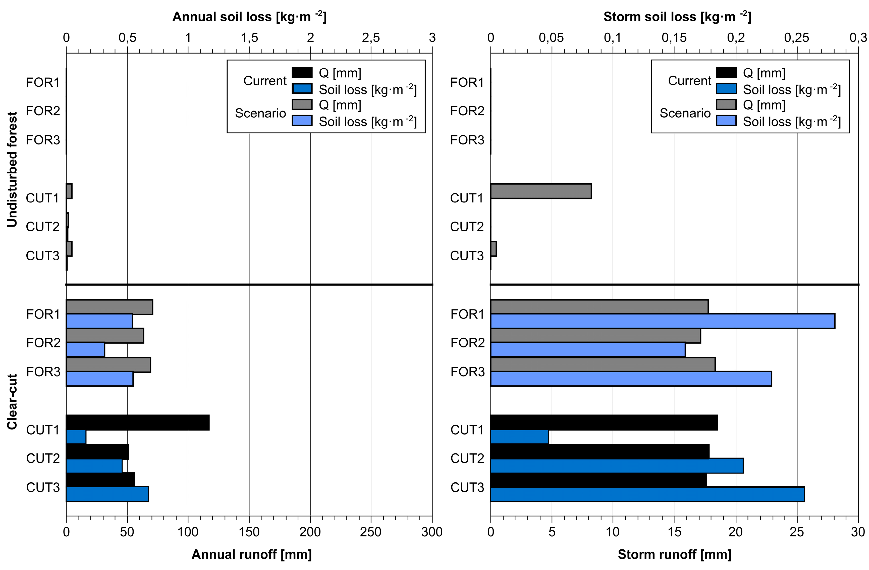
Viewing at FOR, it is clear to see that a future shift from undisturbed forest to clear-cut areas will presumably increase both runoff (+67.69 mm·a−1) and soil erosion (+0.47 kg·m−2·a−1). The same trend is visible when looking at CUT. The actual state shows, that both parameters are increased, compared to the modeled, undisturbed initial situation (+70.99 mm, +0.43 kg·m−2·a−1) (Table 17). Apart from that, the same pattern applies for modeled storm runoff. FOR and CUT show minimal storm runoff and erosion under undisturbed conditions, but clear-cutting leads to a comparable increase of storm runoff, disregarding differing soil and slope properties (Table 18). Storm soil losses are slightly increased with 0.22 kg·m−2·a−1 (FOR) and 0.17 kg·m−2·a−1 (CUT).
SUC and REF allowed modeling both past and future developments. As expected, bare surfaces exhibited the highest annual runoff sums and soil losses (223.43 mm, 7.55 kg·m−2·a−1 (SUC); 190.97 mm, 6.54 kg·m−2·a−1 (REF)). With ongoing succession and forest reestablishment, runoff sums and soil loss become lower (Table 17). These findings reaffirm results obtained during benchmark modeling. This parallelism is even more apparent when viewing at modeled storm results: Major runoff sums were only proven for bare surfaces, accompanied by increased soil erosion rates. Succession and reforestation results show little to no runoff and soil erosion taking place (Table 18).
4. Discussion
There are several constraints making it difficult to categorize the modeling results of this study in the context of other studies. First of all, it is difficult to classify disturbed soils in this study according to common soil classifications like [47]: As they do not meet the requirements of an anthropogenic altered Technosol, some kind of altered Andosol, most likely a “Relocatic Andosol” has to be assumed. This way, the aspect of soil refilling is stated explicitly, but there is still no direct reference to major shifts of soil properties. Compared to other refilled mineral soils, there is not only a disturbance of pedogenetic horizons, but also the removal of its most characteristic feature—volcanic tephra—that has to be considered. Thus, in context of this study, a major effect on runoff generation and therefore soil erosion rates has to be assumed.
Secondly and more importantly, there are currently no existing studies discussing soil erosion for excavated and refilled Andosols. That is why a comparison with other studies is limited to, and focused on runoff/erosion benchmarks derived from undisturbed soils in forested areas on the one hand and land management changes (clear-cutting) on the other hand.
There are studies viewing at soil erosion rates measured and modeled for forest stands in Europe and Germany, overall showing potentially low erosion rates. [48] conducted a comprehensive meta-study assessing soil erosion in Germany. They calculated an average soil loss of 0.02 kg·m−2·a−1, (std. dev. 0.26 kg·m−2·a−1) for forested areas. While forests cover 30% of Germany, according to CORINE land use data, they only contribute roughly 3% of total annual erosion [48]. Another study focusing on a small catchment in the Rhenish Massif modeled erosion rates of 0.07 kg·m−2·a−1 for forests using the empirical USLE model [49]. Recent studies discussing the cover-management factor of USLE [50] also stress the expectably low erosion rates for forests, as mean values for forested areas in Germany are about 100 times lower than those for agricultural land (Cforest = 0.0012, Cagriculture = 0.1219). A study using these factors modeled potential erosion rates of 0.007 kg·m−2·a−1 for forests in Europe [51].
These findings match the modeled results in this study, as mean soil erosion for undisturbed and reestablished forest was only 0.013 kg·m−2·a−1. Therefore, no substantial erosion risk is expectable even after excavation. Yet, this is most likely caused by the beneficial effect of ground cover. Apart from actual vegetation cover, benchmark modeling in this study revealed, that disturbed soils show higher runoff- and soil erosion sums, most likely caused by total conversion due to excavation and refilling. [15] also point out, that-on the basis of prior studies [17,19] — Andosol sites show little to no tendency of soil erosion. However, that it is not only caused by beneficial soil properties e.g., [24,52], but also by the fact that Andosol sites commonly feature a high vegetation cover, thus reducing rainfall erosivity. When it comes to clear-cutting, [22,25] describe, that especially Andosols are comparatively prone to soil erosion. As expected, vegetation removal induced the highest runoff and soil loss sums, both for annual and storm modeling. Mean annual soil losses (7.05 kg·m−2·a−1) show rather serious erosion problems during the first year after excavation. They even equate to standardized erosion on bare fallow land for Germany (7.96 kg·m−2·a−1 according to [48]). These findings are also supported by other studies viewing at post-clear-cutting erosion rates [53,54]. Here, an increase by factor 21 was observed after timber harvesting.
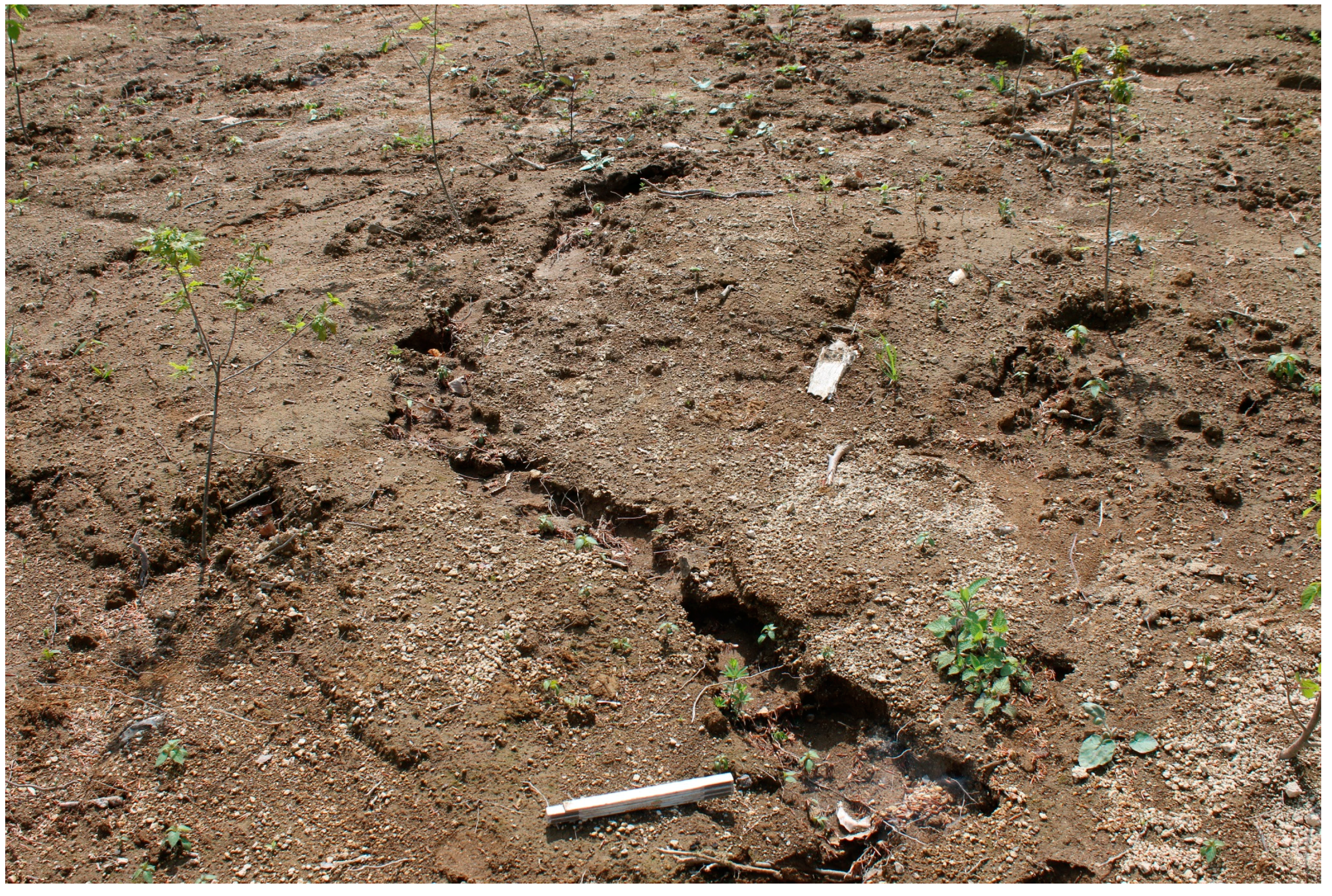
Follow-up inspections on the now bare and refilled sub-area CUT also showed noteworthy erosion processes happening, as there were numerous erosion rills observable (Figure 17).
Fundamentally, major shifts of runoff formation and soil erosion were mostly triggered by land-use change. That is why even the only three-year-old succession site showed no notable soil erosion losses during modeling, even though annual runoff was still increased. Yet, alterations of soil properties caused by refilling were apparently proven. Standardized modeling revealed that these altered soil conditions lead to a higher chance of runoff formation and linked soil erosion processes. Furthermore, changes of soil properties in the aftermath of pumice excavation appear to be at least semi-continuous, as there is no notable statistical difference between soils of sub-areas SUC and REF. Therefore, areas excavated more than 15 years ago show no noticeable sign of recovery.
Yet, the findings of this study can only represent a first-physically based—modeling assumption. While the sophisticated input parameters ensure a most likely realistic magnitude of the modeled processes, a detailed parametrization has to be conducted. That is why sediment traps are currently being installed in the study area and rainfall simulations using the small scale rainfall simulator presented in [20,21] are carried out ongoing. First preliminary results seem to support the modeling results and the complete datasets will be published in future studies.
5. Conclusions
Modeling results clearly showed, that the two observed changes during excavation, land management change and backfilling, have measurable effects concerning runoff formation and soil erosion. Yet, they affect the observed sites in a different temporal extent: Land management change, converting forest stands to clear-cut and bare surfaces showed the most prominent shifts and these changes were also observable during storm modeling. These changes are grave, but they last only about two years, as even succession-areas showed significantly reduced runoff and soil erosion sums. On the other hand, sole backfilling showed less prominent changes during standardized modeling, but these modifications are long-lasting, as the soil structure is altered permanently. Therefore, a fundamental factor governing runoff and soil erosion is being changed and may play a role when it comes to future timber harvesting and/or vegetation removal on previously excavated forest lots. Despite potential future hazards triggered by these changes, it has to be stated that a beneficial and characteristic feature of undisturbed pumice Andosols, rare runoff formation and soil erosion events, is being disturbed severely by excavation and backfilling—most likely permanently.
Author Contributions
Conceptualization, J.J.Z.; methodology, J.J.Z.; validation, J.J.Z., J.P. and S.S.; formal analysis, J.J.Z., J.P. and S.S.; investigation, J.J.Z., J.P. and S.S.; resources, J.J.Z.; data curation, J.J.Z., J.P. and S.S.; writing—original draft preparation, J.J.Z.; writing—review and editing, J.J.Z.; visualization, J.J.Z.; supervision, J.J.Z.
Funding
This research received no external funding.
Acknowledgments
We would like to thank Johannes Biwer, forester in the Bendorf forest district, for his help and constructive input during data sampling and for providing detailed information about tree populations and past excavation works. Also, we would like Alexander Klein for providing two photographs of the study site.
Conflicts of Interest
The authors declare no conflict of interest.
References
- Baales, M.; Jöris, O.; Street, M.; Bittmann, F.; Weninger, B.; Wiethold, J. Impact of the Late Glacial Eruption of the Laacher See Volcano, Central Rhineland, Germany. Quat. Res. 2002, 58, 273–288. [Google Scholar] [CrossRef]
- Schmincke, H.-U.; Park, C.; Harms, E. Evolution and environmental impacts of the eruption of Laacher See Volcano (Germany) 12,900 a BP. Quat. Int. 1999, 61, 61–72. [Google Scholar] [CrossRef]
- Riede, F.; Bazely, O.; Newton, A.J.; Lane, C.S. A Laacher See-eruption supplement to Tephrabase: Investigating distal tephra fallout dynamics. Quat. Int. 2011, 246, 134–144. [Google Scholar] [CrossRef]
- Brauer, A.; Endres, C.; Negendank, J.F.W. Lateglacial calendar year chronology based on annually laminated sediments from Lake Meerfelder Maar, Germany. Quat. Int. 1999, 61, 17–25. [Google Scholar] [CrossRef]
- Bogaard, P.v.d. Ar-40/Ar-39 ages of Sanidine phenocrysts from Laacher-See-tephra (12,900 Yr BP)—Chronostratigraphic and petrological significance. Earth Planet. Sci. Lett. 1995, 133, 163–174. [Google Scholar] [CrossRef]
- Kleber, M.; Jahn, R. Andosols and soils with andic properties in the German soil taxonomy. J. Plant Nutr. Soil Sci. 2007, 170, 317–328. [Google Scholar] [CrossRef]
- Rennert, T.; Eusterhues, K.; Hiradate, S.; Breitzke, H.; Buntkowsky, G.; Totsche, K.U.; Mansfeldt, T. Characterisation of Andosols from Laacher See tephra by wet-chemical and spectroscopic techniques (FTIR, 27Al-, 29Si-NMR). Chem. Geol. 2014, 363, 13–21. [Google Scholar] [CrossRef]
- Kleber, M.; Mikutta, C.; Jahn, R. Andosols in Germany—Pedogenesis and properties. Catena 2004, 56, 67–83. [Google Scholar] [CrossRef]
- Jimènez, C.C.; Tejedor, M.; Morillas, G.; Neris, J. Infiltration rate of andisols: Effect of changes in vegetation cover (Tenerife, Spain). J. Soil Water Conserv. 2006, 61, 153–158. [Google Scholar]
- Neris, J.; Jimènez, C.; Fuentes, J.; Morillas, G.; Tejedor, M. Vegetation and land-use effects on soil properties and water infiltration of Andisols in Tenerife (Canary Islands, Spain). Catena 2012, 98, 55–62. [Google Scholar] [CrossRef]
- Tejedor, M.; Neris, J.; Jimènez, C. Soil properties controlling infiltration in volcanic soils (Tenerife, Spain). Soil Sci. Soc. Am. J. 2012, 77, 202–212. [Google Scholar] [CrossRef]
- Neris, J.; Tejedor, M.; Rodríguez, M.; Fuentes, J.; Jiménez, C. Effect of forest floor characteristics on water repellency, infiltration, runoff and soil loss in Andisols of Tenerife (Canary Islands, Spain). Catena 2013, 108, 50–57. [Google Scholar] [CrossRef]
- Nanzyo, M.; Shoji, S.; Dahlgren, R. Physical characteristics of volcanic ash soils. In Volcanic Ash Soils: Genesis, Properies and Utilization; Shoji, S., Nazyo, M., Dahlgren, R., Eds.; Elsevier Science Publishers: Amsterdam, The Netherlands, 1993; p. 288. [Google Scholar]
- Orradottir, B.; Archer, S.R.; Arnalds, O.; Wilding, L.P.; Thurow, T.L. Infiltration in Icelandic Andisols: The role of vegetation and soil frost. Arct. Antarct. Alp. Res. 2008, 40, 412–421. [Google Scholar] [CrossRef]
- Rodríguez Rodríguez, A.; Guerra, J.A.; Gorrín, S.P.; Arbelo, C.D.; Mora, J.L. Aggregates stability and water erosion in Andosols of the Canary Islands. Land Degrad. Dev. 2002, 13, 515–523. [Google Scholar] [CrossRef]
- Rodríguez Rodríguez, A.; Arbelo, C.D.; Guerra, J.A.; Mora, J.L.; Notario, J.S.; Armas, C.M. Organic carbon stocks and soil erodibility on Canary Islands Andosols. Catena 2006, 66, 228–235. [Google Scholar] [CrossRef]
- Khamsouk, B.; Roose, E.; Dorel, M.; Blanchart, E. Effect des systèmes de culture bananière sur la stabilité structurale et l’érosion d’un solrouille à halloysite en Martinique. Bull. Rés. Eros. 1999, 19, 206–215. [Google Scholar]
- Khamsouk, B.; De Noni, G.; Roose, E. New Data Concerning Erosion Processes and Soil Management on Andosols from Ecuador and Martinique. In Proceedings of the 12th ISCO Conference 2002, Beijing, China, 26–31 May 2002. [Google Scholar]
- Roose, E.; Khamsouk, B.; Lassoudiere, A.; Dorel, M. Origine du ruisselement et de l’érosion sur sols bruns à halloysite de Martinique. Premières observations sous bananiers. Bull. Réseau Eros. 1999, 19, 139–147. [Google Scholar]
- Zemke, J.J. Runoff and Soil Erosion Assessment on Forest Roads Using a Small Scale Rainfall Simulator. Hydrology 2016, 3, 25. [Google Scholar] [CrossRef]
- Zemke, J.J.; Enderling, M.; Klein, A.; Skubski, M. The Influence of Soil Compaction on Runoff Formation. A Case Study Focusing on Skid Trails at Forested Andosol Sites. Geosciences 2019, 9, 204. [Google Scholar] [CrossRef]
- Arnalds, O.; Þorarinsdottir, E.F.; Metusalemsson, S.; Jonsson, A.; Gretarsson, E.; Arnason, A. Soil Erosion in Iceland; Soil Conservation Service and the Agricultural Research Institute: Reykjavík, Iceland, 2001. [Google Scholar]
- Page-Dumroese, D.; Miller, R.; Mital, J.; McDaniel, P.; Miller, D. Volcanic-Ash-Derived Forest Soils of the Inland Northwest: Properties and Implications for Management and Restoration. In Proceedings RMRS-P-44; U.S. Department of Agriculture, Forest Service, Rocky Mountain Research Station: Fort Collins, CO, USA, 2007. [Google Scholar]
- McDaniel, P.A.; Wilson, M.A. Physical and Chemical Characteristics of Ash-influenced Soils of Inland Northwest Forests. In Volcanic-Ash-Derived Forest Soils of the Inland Northwest: Properties and Implications for Management and Restoration; Page-Dumroese, D., Miller, R., Mital, J., McDaniel, P., Miller, D., Eds.; Rocky Mountain Research Station: Fort Collins, CO, USA, 2007. [Google Scholar]
- Kimble, J.M.; Ping, C.L.; Sumner, M.E.; Wilding, L.P. Classification of Soils: Andisols. In Handbook of Soil Science; Sumner, M.E., Ed.; CRC Press: New York, NY, USA, 2000. [Google Scholar]
- Geist, J.M.; Cochran, P.H. Influences of volcanic ash and pumice deposition on productivity of western interior forest soils. In Proceedings—Management and Productivity of Western-Montane Forest Soils; Harvey, A.E., Neuenschwander, L.F., Eds.; Intermountain Research Station General Technical Report, INT-280; Intermountain Research Station: Ogden, UT, USA, 1991. [Google Scholar]
- Blume, T.; Zehe, E.; Reusser, D.; Bauer, A.; Iroume, A.; Bonstert, A. Investigation of runoff generation in a pristine, poorly gauged catchment in the Chilean Andes. I: A multi-method experimental study. Hydrol. Proc. 2008, 22, 3661–3675. [Google Scholar] [CrossRef]
- Blume, T.; Zehe, E.; Bronstert, A. Investigation of runoff generation in a pristine, poorly gauged catchment in the Chilean Andes. II: Qualitative and quantitative use of tracers at three different spatial scales. Hydrol. Proc. 2008, 22, 3676–3688. [Google Scholar] [CrossRef]
- Blume, T.; Zehe, E.; Bronstert, A. Use of soil moisture dynamics and patterns at different spatio-temporal scales for the investigation of subsurface flow processes. Hydrol. Earth Syst. Sci. 2009, 13, 1215–1234. [Google Scholar] [CrossRef]
- Laflen, J.M.; Lane, L.J.; Foster, G.R. WEPP A new generation of erosion prediction technology. J. Soil Water Conversat. 1991, 46, 34–38. [Google Scholar]
- Flanagan, D.C.; Nearing, M.A. Water Erosion Prediction Project Hillslope Project and Watershed Model Documentation; NSERL Report No. 10; NSERL: West Lafayette, IN, USA, 1995. [Google Scholar]
- Flanagan, D.C.; Fu, H.; Frankenberger, J.R.; Livingston, S.J.; Meyer, C.R. A Windows Interface for the WEPP Erosion Model; ASAE Paper No. 982135; ASAE Paper: St Joseph, MI, USA, 1998. [Google Scholar]
- Flanagan, D.C.; Gilley, J.E.; Franti, T.G. Water Erosion Prediction Project (WEPP): Development history, model capabilities, and future enhancements. Trans. Am. Soc. Agric. Bio. Eng. 2007, 50, 1603–1612. [Google Scholar] [CrossRef]
- Laflen, J.M.; Flanagan, D.C. The development of U.S. soil erosion prediction and modeling. Int. Soil Water Conserv. Res. 2013, 1, 1–11. [Google Scholar] [CrossRef]
- Elliot, W.J.; Hall, D.E. Water Erosion Prediction Project (WEPP) Forest Applications; Intermountain Research Station General Technical Report Draft: Ogden, UT, USA, 1997. [Google Scholar]
- Covert, A.; Robichaud, P.R.; Elliot, W.J.; Link, T.E. Evaluation of Runoff Prediction from WEPP-based Erosion Models for Harvested and Burned Forest Watersheds. Trans. ASAE 2005, 48, 1091–1100. [Google Scholar] [CrossRef]
- Elliot, W.J. WEPP Internet Interfaces for Forest Erosion Prediction. J. Am. Water Resour. Assoc. 2007, 40, 299–309. [Google Scholar] [CrossRef]
- Dun, S.; Wu, J.Q.; Elliot, W.J.; Robichaud, P.R.; Flanagan, D.C.; Frankenberger, J.R.; Brown, R.E.; Xu, A.C. Adapting the Water Erosion Prediction Project (WEPP) model for forest applications. J. Hydrol. 2009, 366, 46–54. [Google Scholar] [CrossRef]
- Zemke, J.J. Messung, Simulation und Modellierung von Oberflächenabfluss und Bodenabtrag auf Wirtschaftswegen in bewaldeten Einzugsgebieten. Ph.D. Thesis, University Koblenz-Landau, Koblenz, Mainz, Germany, 2015. [Google Scholar]
- Meyer, C. General Description of the CLIGEN Model and Its History; USDA-ARS National Soil Erosion Laboratory: West Lafayette, IN, USA, 2011. Available online: https://www.ars.usda.gov/ARSUserFiles/50201000/WEPP/cligen/CLIGENDescription.pdf (accessed on 30 July 2019).
- Mueller, E.N.; Pfister, A. Increasing occurence of high-intensity rainstorm events relevant for the generation of soil erosion in a temperate lowland region in Central Europe. J. Hydrol. 2011, 411, 266–278. [Google Scholar] [CrossRef]
- Bilotta, G.S.; Krueger, T.; Brazier, R.E.; Butler, P.; Freer, J.; Hawkins, J.M.B.; Haygarth, P.M.; Macleod, C.J.A.; Quinton, J.N. Assessing catchment-scale erosion and yields of suspended solids from improved temperate grassland. J. Environ. Monit. 2010, 12, 731–739. [Google Scholar] [CrossRef]
- Morgan, R.P.C. Soil Erosion and Conservation; Blackwell Publishing: Malden, MA, USA, 2005. [Google Scholar]
- Flanagan, D.C.; Livingston, S.J. WEPP User Summary; National Soil Erosion Research Laboratory Report No. 11; National Soil Erosion Research Laboratory Report: West Lafayette, IN, USA, 1995. [Google Scholar]
- Ad-Hoc-Arbeitsgruppe Boden. Bodenkundliche Kartieranleitung, 5th ed.; E.Schweizerbart’sche Verlagsbuchandlung: Stuttgart, Germany, 2005. [Google Scholar]
- Cohen, J. Statistical Power Analysis for the Behavioral Sciences; Taylor and Francis: Milton Park, UK, 1988. [Google Scholar]
- Food and Agriculture Organization of the United Nations (FAO). World Reference Base for Soil Resources 2014: International Soil Classification System for Naming Soils and Creating Legends for Soil Maps—Update 2015; FAO: Rome, Italy, 2015; pp. 146–147. [Google Scholar]
- Auerswald, K.; Fiener, P.; Dikau, R. Rates of sheet and rill erosion in Germany—A meta-analysis. Geoorphology 2009, 111, 182–193. [Google Scholar] [CrossRef]
- Hacisalihoglu, S. Determination of soil erosion in a steep hill slope with different land-use types: A case study in Mertesdorf (Ruwertal/Germany). J. Einviron. Biol. 2007, 28, 433–438. [Google Scholar]
- Panagos, P.; Borrelli, P.; Meusburger, K.; Alewell, C.; Lugato, E.; Montanarella, L. Estimating the soil erosion cover-management factor at the European scale. Land Use Policy 2015, 48, 38–50. [Google Scholar] [CrossRef]
- Panagos, P.; Borrelli, P.; Poesen, J.; Ballabio, C.; Lugato, E.; Meusburger, K.; Montanarella, L.; Alewell, C. The new assessment of soil loss by water erosion in Europe. Environ. Sci. Policy 2015, 54, 438–447. [Google Scholar] [CrossRef]
- Meurisse, R.T. Properties of Andisols important to forestry. In Taxonomy and Management of Andisols, Proceedings of the Sixth International Soil Classification Workshop, Chile and Ecuador, Santiago de Chile, Chile, 9–20 January 1984; Sociedad Chilena de la Ciencia del Suelo: Santiago, Chile, 1985; pp. 53–67. [Google Scholar]
- Borrelli, P.; Schütt, B. Assessment of soil erosion sensitivity and post-timber-harvesting erosion response in a mountain environment of Central Italy. Geomorphology 2014, 204, 412–424. [Google Scholar] [CrossRef]
- Borrelli, P.; Panagos, P.; Märker, M.; Modugno, S.; Schütt, B. Assessment of the impacts of clear-cutting on soil loss by water erosion in Italian forests: First comprehensive monitoring and modelling approach. Catena 2017, 149, 770–781. [Google Scholar] [CrossRef]
Figure 1.
Pumice excavation in forest district Bendorf, 2018 (Photo: Alexander Klein). Material for later backfilling is visible on both sides.
Figure 1.
Pumice excavation in forest district Bendorf, 2018 (Photo: Alexander Klein). Material for later backfilling is visible on both sides.
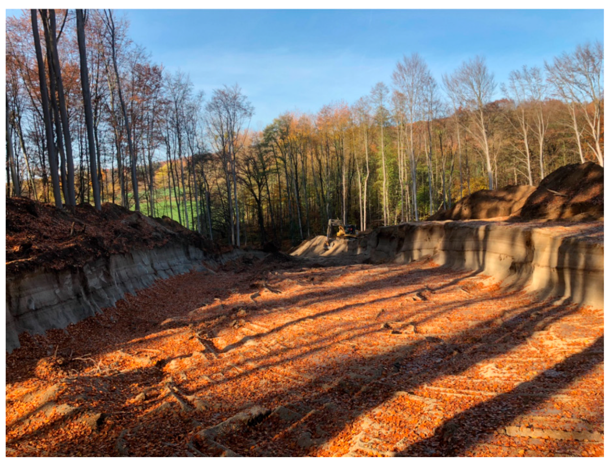
Figure 2.
Location of the study area, after [21].
Figure 2.
Location of the study area, after [21].
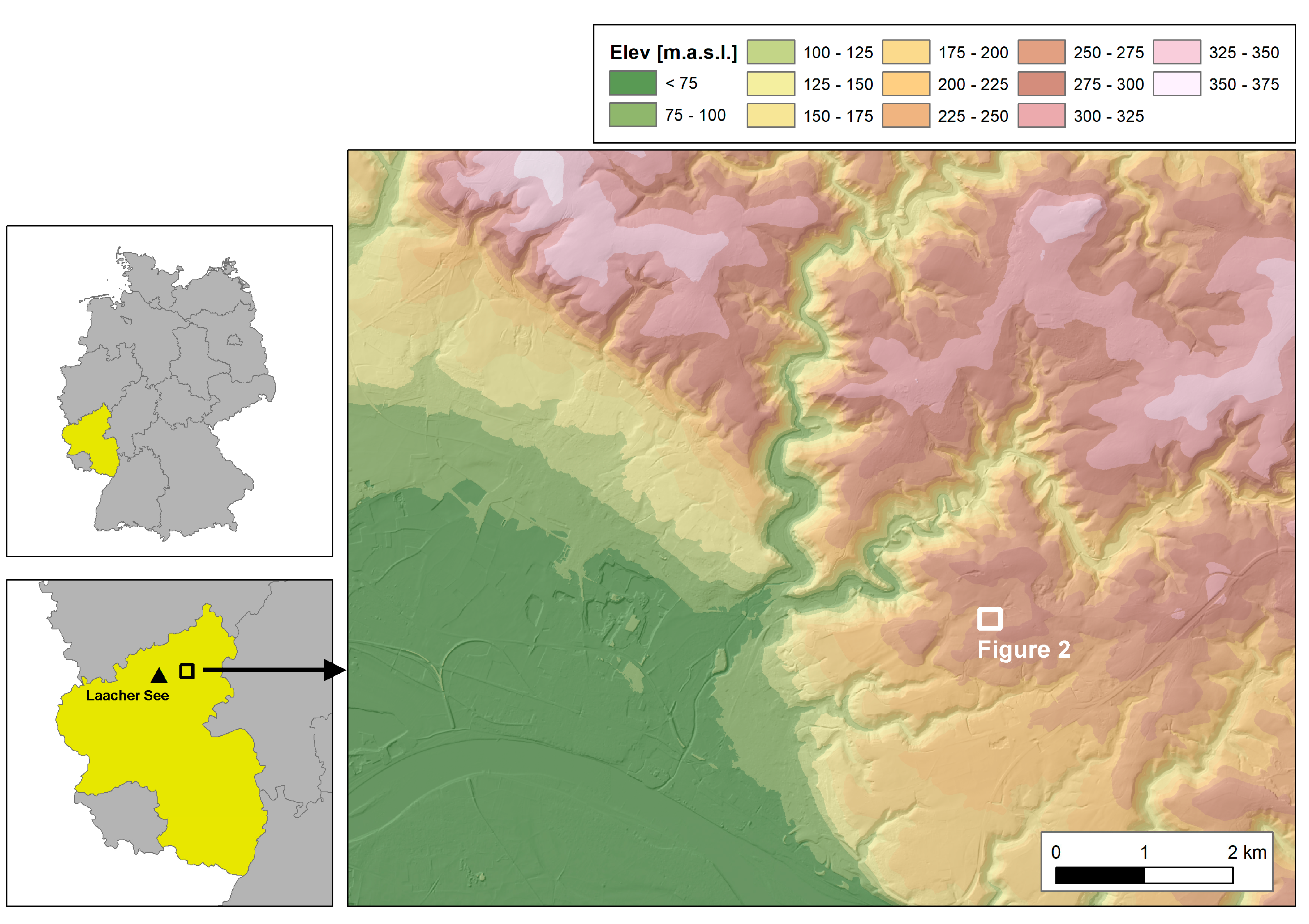
Figure 3.
Study area, sampling point and catenae indicated. Catena labels refer to sub-areas: (FOR)ested, (CUT)-down, (SUC)cession, (REF)orested. Aerial photography by the Land Surveying State Office of Rhineland-Palatinate.
Figure 3.
Study area, sampling point and catenae indicated. Catena labels refer to sub-areas: (FOR)ested, (CUT)-down, (SUC)cession, (REF)orested. Aerial photography by the Land Surveying State Office of Rhineland-Palatinate.

Figure 4.
Climograph for weather station Grenzau, raw data collected by the Dienstleistungszentrum Ländlicher Raum Rhineland-Palatinate.
Figure 4.
Climograph for weather station Grenzau, raw data collected by the Dienstleistungszentrum Ländlicher Raum Rhineland-Palatinate.

Figure 5.
Slope geometry for every catena; (FOR)est, (CUT)-down, (SUC)cession, (REF)forested.

Figure 6.
Land management stages: (a) undisturbed forest, (b) clear-cut, (c) excavation works, (d) bare surface, (e) succession, (f) reestablished forest. (Photo 4 (b): Alexander Klein). (b–d) show excavation works on the same sub-area.
Figure 6.
Land management stages: (a) undisturbed forest, (b) clear-cut, (c) excavation works, (d) bare surface, (e) succession, (f) reestablished forest. (Photo 4 (b): Alexander Klein). (b–d) show excavation works on the same sub-area.
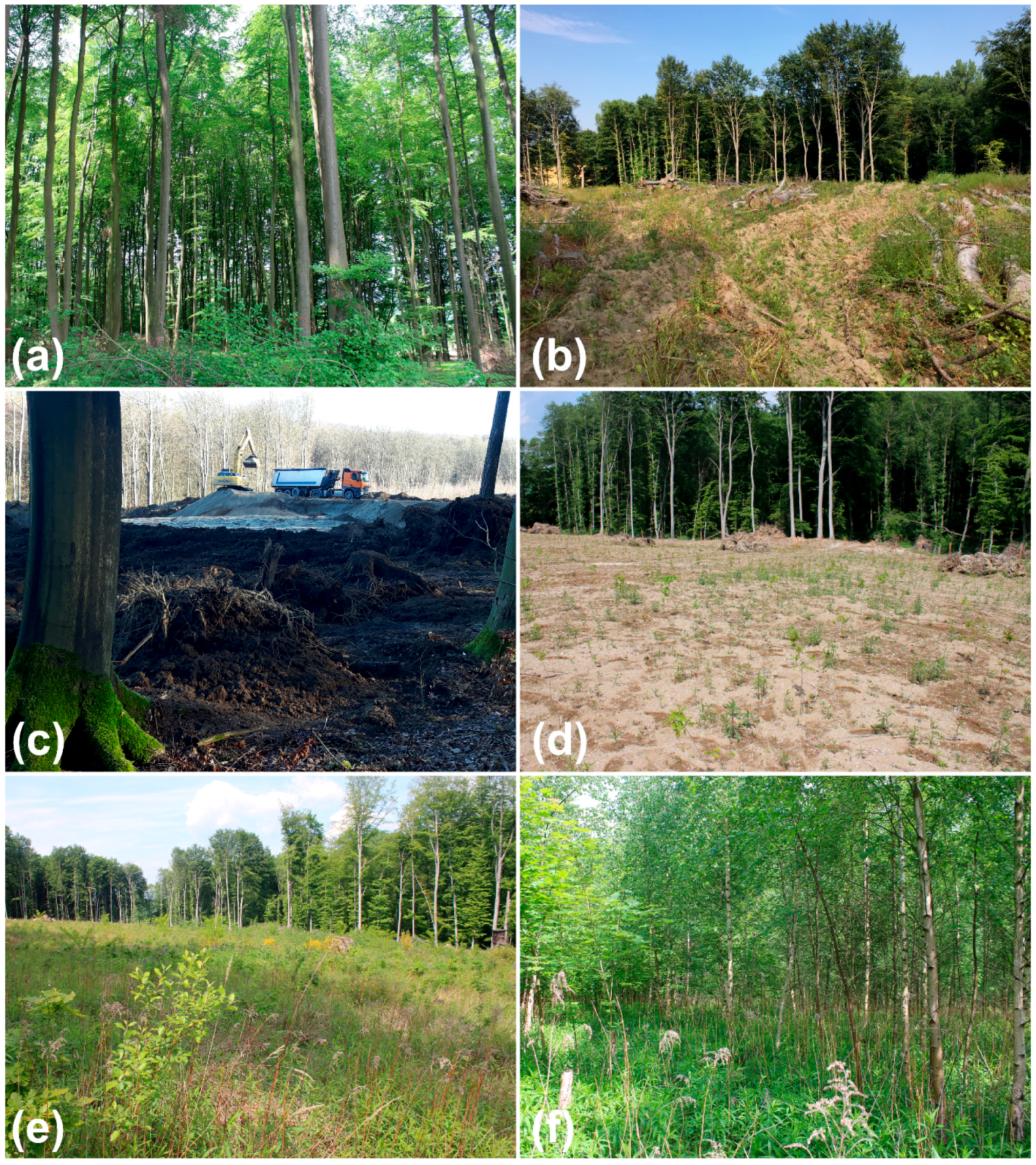
Figure 7.
Depth-related sand content for every catena: (FOR)est, (CUT)-down, (SUC)cession, (REF)forested; solid line: upper slope, dashed line: middle slope, dotted line: lower slope.
Figure 7.
Depth-related sand content for every catena: (FOR)est, (CUT)-down, (SUC)cession, (REF)forested; solid line: upper slope, dashed line: middle slope, dotted line: lower slope.

Figure 8.
Depth-related clay content for every catena: (FOR)est, (CUT)-down, (SUC)cession, (REF)forested; solid line: upper slope, dashed line: middle slope, dotted line: lower slope.
Figure 8.
Depth-related clay content for every catena: (FOR)est, (CUT)-down, (SUC)cession, (REF)forested; solid line: upper slope, dashed line: middle slope, dotted line: lower slope.

Figure 9.
Depth-related SOM content for every catena: (FOR)est, (CUT)-down, (SUC)cession, (REF)forested; solid line: upper slope, dashed line: middle slope, dotted line: lower slope.
Figure 9.
Depth-related SOM content for every catena: (FOR)est, (CUT)-down, (SUC)cession, (REF)forested; solid line: upper slope, dashed line: middle slope, dotted line: lower slope.
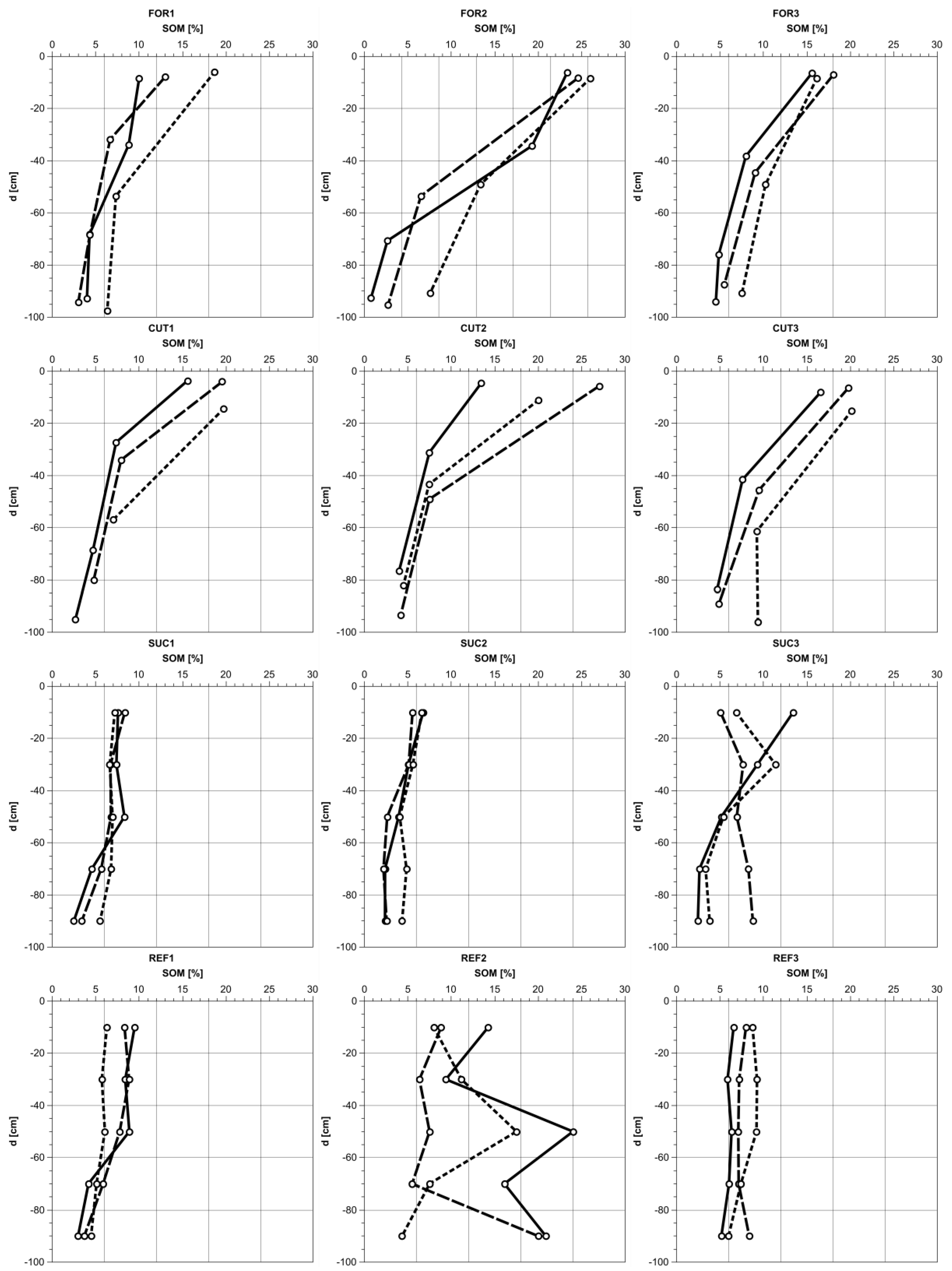
Figure 10.
Depth-related CEC content for every catena: (FOR)est, (CUT)-down, (SUC)cession, (REF)forested; solid line: upper slope, dashed line: middle slope, dotted line: lower slope.
Figure 10.
Depth-related CEC content for every catena: (FOR)est, (CUT)-down, (SUC)cession, (REF)forested; solid line: upper slope, dashed line: middle slope, dotted line: lower slope.

Figure 11.
Dataset distribution of standardized modeling for disturbed and undisturbed soils, viewing at singular soil samples.
Figure 11.
Dataset distribution of standardized modeling for disturbed and undisturbed soils, viewing at singular soil samples.
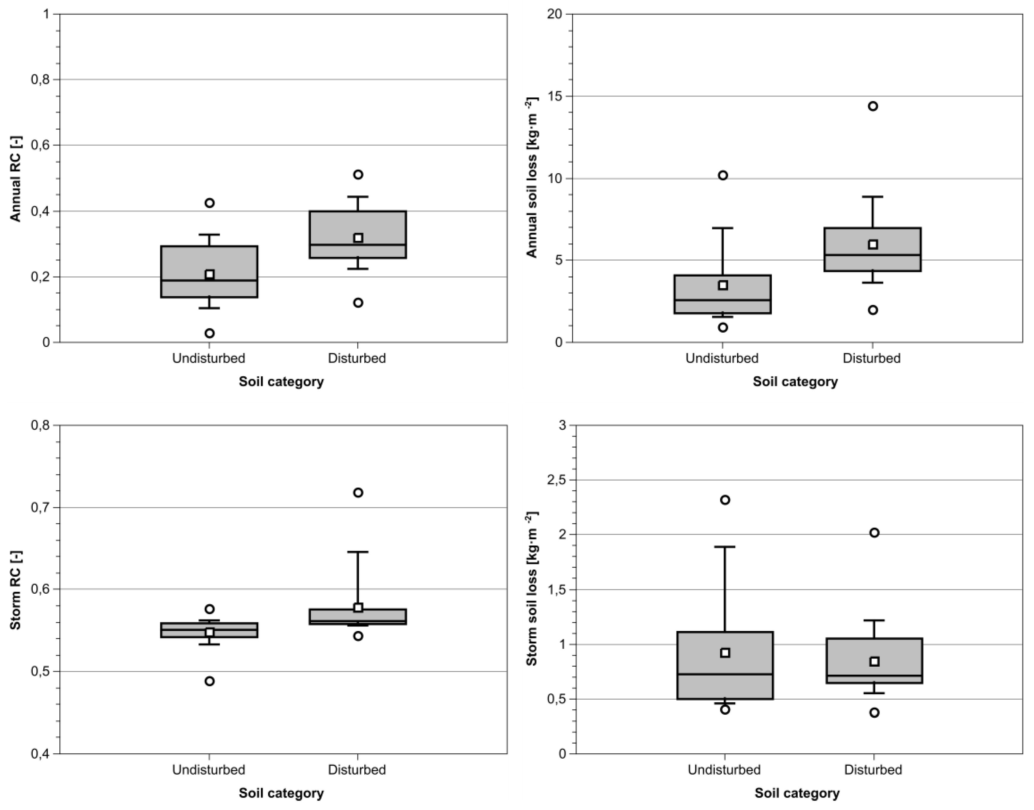
Figure 12.
Dataset distribution of standardized modeling for every sub-area, viewing at singular soil samples; (FOR)est, (CUT)-down, (SUC)cession, (REF)forested.
Figure 12.
Dataset distribution of standardized modeling for every sub-area, viewing at singular soil samples; (FOR)est, (CUT)-down, (SUC)cession, (REF)forested.

Figure 13.
Modeling results for land management shifts on standardized slope, annual runoff coefficient (RC) and soil loss. Y-error indicates standard deviation, blue columns indicate undisturbed soils, red columns indicate disturbed soils.
Figure 13.
Modeling results for land management shifts on standardized slope, annual runoff coefficient (RC) and soil loss. Y-error indicates standard deviation, blue columns indicate undisturbed soils, red columns indicate disturbed soils.
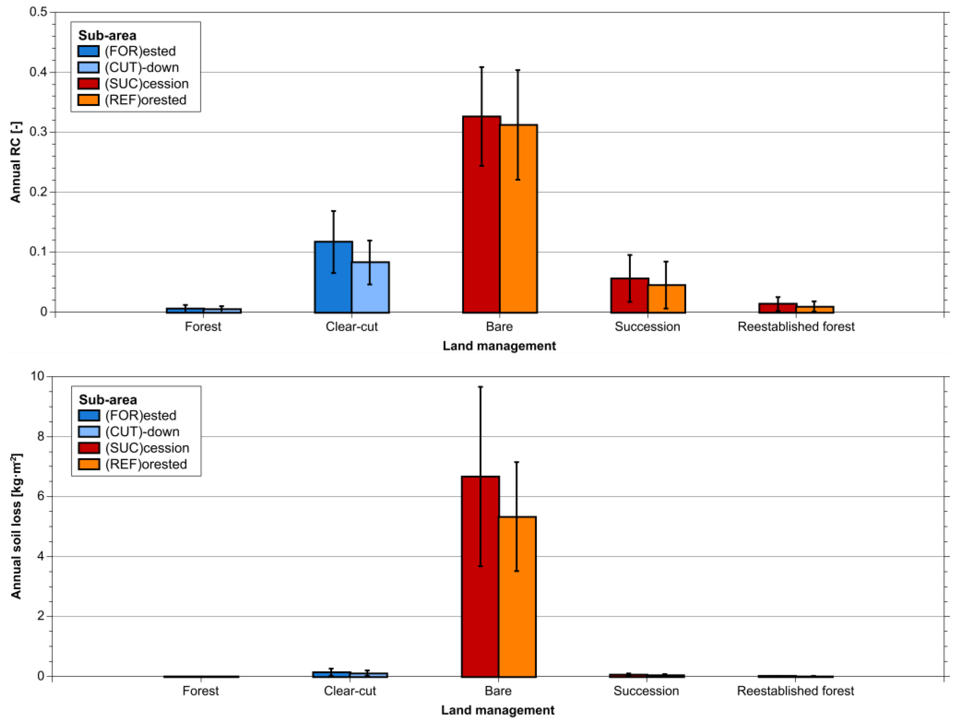
Figure 14.
Modeling results for land management shifts on standardized slope, storm runoff coefficient (RC) and soil loss. Y-error indicates standard deviation, blue columns indicate undisturbed soils, red columns indicate disturbed soils.
Figure 14.
Modeling results for land management shifts on standardized slope, storm runoff coefficient (RC) and soil loss. Y-error indicates standard deviation, blue columns indicate undisturbed soils, red columns indicate disturbed soils.
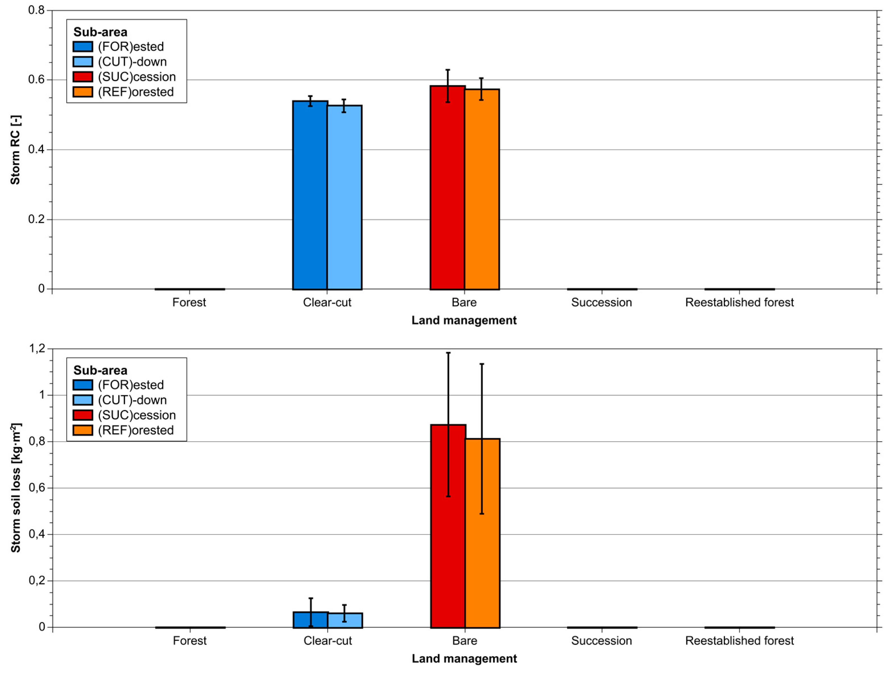
Figure 15.
Modeling results (annual and storm) for (FOR)ested and (CUT)-down sites, using realistic slope geometry and different land managements.
Figure 15.
Modeling results (annual and storm) for (FOR)ested and (CUT)-down sites, using realistic slope geometry and different land managements.

Figure 16.
Modeling results (annual and storm) for (SUC)cession and (REF)orested sites, using realistic slope geometry and different land managements.
Figure 16.
Modeling results (annual and storm) for (SUC)cession and (REF)orested sites, using realistic slope geometry and different land managements.

Figure 17.
Example for an erosion rill on backfilled sub-area CUT, folding ruler for scale.

Table 1.
Climate data used for Water Erosion Prediction Project (WEPP) modeling, excerpt from CLIGEN parameter file.
Table 1.
Climate data used for Water Erosion Prediction Project (WEPP) modeling, excerpt from CLIGEN parameter file.
| Parameter | Jan. | Feb. | Mar. | Apr. | May | Jun. | Jul. | Aug. | Sep. | Oct. | Nov. | Dec. |
|---|---|---|---|---|---|---|---|---|---|---|---|---|
| Avg. P [mm] | 38.7 | 29.6 | 47.2 | 45.3 | 56.4 | 61.2 | 56.3 | 50.6 | 40.2 | 40.0 | 47.2 | 48.6 |
| No. of wet days | 16.9 | 11.7 | 15.5 | 12.7 | 13.1 | 13.4 | 12.3 | 10.5 | 11.3 | 12.1 | 14.3 | 16.0 |
| Max 30 min P [mm] | 7.1 | 8.1 | 4.3 | 5.6 | 10.2 | 11.0 | 9.4 | 10.7 | 6.9 | 6.4 | 6.4 | 6.6 |
| Avg.Tmax [°C] | 4.0 | 5.3 | 10.4 | 13.9 | 18.8 | 21.2 | 23.7 | 23.8 | 20.2 | 15.0 | 8.4 | 5.7 |
| Avg. Tmin [°C] | 0.5 | 0.0 | 3.8 | 5.4 | 9.3 | 12.6 | 14.3 | 14.2 | 11.8 | 8.6 | 4.2 | 2.3 |
Table 2.
Slope parameters for every catena; (FOR)est, (CUT)-down, (SUC)cession, (REF)forested.
| Catena | Length [m] | Mean Slope [%] |
|---|---|---|
| FOR1 | 130.5 | 9.01 |
| FOR2 | 123.1 | 9.98 |
| FOR3 | 105.35 | 12.58 |
| CUT1 | 86.81 | 15.05 |
| CUT2 | 99.19 | 14.62 |
| CUT3 | 107.07 | 13.65 |
| SUC1 | 63.36 | 8.74 |
| SUC2 | 62.60 | 12.88 |
| SUC3 | 62.26 | 11.82 |
| REF1 | 80.44 | 9.92 |
| REF2 | 95.67 | 9.33 |
| REF3 | 89.45 | 4.25 |
| Ø | 92.15 | 10.99 |
Table 3.
Land-management stages defined for modeling.
| Land-Management | FOR | CUT | SUC | REF |
|---|---|---|---|---|
| Undisturbed forest | Current | Scenario | - | - |
| Clear-cut with understory vegetation | Scenario | Current | - | - |
| Clear-cut without understory vegetation | Scenario | Current | - | - |
| Bare surface | - | - | Scenario | Scenario |
| Succession | - | - | Current | Scenario |
| Reestablished forest | - | - | Scenario | Current |
Table 4.
Land-management stages and WEPP presets used.
| Land-Management | Preset |
|---|---|
| Undisturbed forest | Forest perennial |
| Clear-cut | Altered preset, starting with disturbed forest and 90% ground cover. Disturbance on Sep 1st, removing ground cover |
| Bare surface | Fallow |
| Succession | Tall grass prairie |
| Reestablished forest | Tree 20yr forest |
Table 5.
Significance (p) and effect size (η2), testing depth- and soil-related influence on soil parameters (Two-way ANOVA for soil categories undisturbed and disturbed). Significant values appear bold.
Table 5.
Significance (p) and effect size (η2), testing depth- and soil-related influence on soil parameters (Two-way ANOVA for soil categories undisturbed and disturbed). Significant values appear bold.
| Sand [%] | Clay [%] | SOM [%] | CEC [meq·(100 g)−1] | |||||
|---|---|---|---|---|---|---|---|---|
| p | η2 | p | η2 | p | η2 | p | η2 | |
| Soil category | 0.67 | 0.00 | 0.19 | 0.01 | <0.05 | 0.14 | <0.05 | 0.12 |
| Depth | <0.05 | 0.05 | <0.05 | 0.04 | <0.05 | 0.47 | <0.05 | 0.45 |
| Soil category * depth | <0.05 | 0.18 | <0.05 | 0.14 | <0.05 | 0.28 | <0.05 | 0.26 |
Table 6.
Significance (p) and effect size (η2), testing depth- and soil-related influence on soil parameters (Two-way ANOVA for soil categories FOR, CUT, SUC and REF). Significant values appear bold.
Table 6.
Significance (p) and effect size (η2), testing depth- and soil-related influence on soil parameters (Two-way ANOVA for soil categories FOR, CUT, SUC and REF). Significant values appear bold.
| Sand [%] | Clay [%] | SOM [%] | CEC [meq·(100 g)−1] | |||||
|---|---|---|---|---|---|---|---|---|
| p | η2 | p | η2 | p | η2 | p | η2 | |
| Soil category | 0.52 | 0.01 | <0.05 | 0.03 | <0.05 | 0.15 | <0.05 | 0.13 |
| Depth | <0.05 | 0.05 | <0.05 | 0.04 | <0.05 | 0.49 | <0.05 | 0.46 |
| Soil category * depth | <0.05 | 0.20 | <0.05 | 0.17 | <0.05 | 0.30 | <0.05 | 0.28 |
Table 7.
Rock content of every catena; (FOR)ested, (CUT)-down, (SUC)cession, (REF)orested.
| n | Mean Rock [%] | |
|---|---|---|
| FOR1 | 10 | 10.9 |
| FOR2 | 10 | 10.2 |
| FOR3 | 9 | 13.7 |
| CUT1 | 8 | 8.7 |
| CUT2 | 10 | 11.7 |
| CUT3 | 10 | 10.6 |
| SUC1 | 10 | 8.6 |
| SUC2 | 10 | 9.4 |
| SUC3 | 10 | 11.9 |
| REF1 | 10 | 8.1 |
| REF2 | 10 | 8.9 |
| REF3 | 10 | 8.4 |
Table 8.
Mean topsoil texture, erodibilities, critical shear stress and effective hydraulic conductivity (Keff) and mean site-specific effective hydraulic conductivity of every sub-area; (FOR)ested, (CUT)-down, (SUC)cession, (REF)orested.
Table 8.
Mean topsoil texture, erodibilities, critical shear stress and effective hydraulic conductivity (Keff) and mean site-specific effective hydraulic conductivity of every sub-area; (FOR)ested, (CUT)-down, (SUC)cession, (REF)orested.
| FOR | CUT | SUC | REF | |
|---|---|---|---|---|
| Mean topsoil clay [%] | 21.8 | 13.9 | 14.2 | 18.5 |
| Mean topsoil silt [%] | 42.4 | 50.4 | 22.8 | 24.9 |
| Mean topsoil sand [%] | 36.0 | 36.1 | 63.0 | 56.6 |
| Mean topsoil texture (FAO) | Loam | Silt loam | Sandy loam | Sandy loam |
| Mean topsoil interrill erodibility [kg·s·(m−4)−1] | 8,298,158 | 8,152,953 | 10,193,226 | 9,831,884 |
| Mean topsoil rill erodibility [s·m−1] | 0.0157 | 0.0164 | 0.0143 | 0.0144 |
| Mean topsoil critical shear stress [N·m−2] | 2.22 | 2.08 | 1.26 | 0.68 |
| Mean topsoil Keff [mm·h−1] | 10.04 | 10.90 | 21.26 | 18.90 |
| Mean site-specific Keff [mm·h−1] | 1.17 | 2.11 | 0.68 | 0.75 |
Table 9.
Descriptive statistics for standardized modeling results undisturbed and disturbed samples.
Table 9.
Descriptive statistics for standardized modeling results undisturbed and disturbed samples.
| Undisturbed | Disturbed | |
|---|---|---|
| n | 57 | 60 |
| Mean annual runoff [mm] | 142.54 | 217.41 |
| Mean annual RC [-] | 0.21 | 0.32 |
| Mean annual soil loss [kg·m−2] | 3.52 | 5.99 |
| Mean storm runoff [mm] | 18.37 | 19.38 |
| Mean storm RC [-] | 0.55 | 0.58 |
| Mean storm soil loss [kg·m−2] | 0.92 | 0.84 |
Table 10.
Results of Mann-Whitney U-test, testing differences between undisturbed and disturbed samples.
Table 10.
Results of Mann-Whitney U-test, testing differences between undisturbed and disturbed samples.
| Annual Runoff | Annual Soil Loss | Storm Runoff | Storm Soil Loss | |
|---|---|---|---|---|
| p | 2.4 × 10⁻⁸ * | 6.5 × 10⁻⁹ * | 5.1 × 10⁻¹⁰ * | 0.754 |
* Significantly different (p < 0.05).
Table 11.
Descriptive statistics of standardized modeling results for individual land-management categories: (FOR)ested, (CUT)-down, (SUC)cession and (REF)orested.
Table 11.
Descriptive statistics of standardized modeling results for individual land-management categories: (FOR)ested, (CUT)-down, (SUC)cession and (REF)orested.
| FOR | CUT | SUC | REF | |
|---|---|---|---|---|
| n | 29 | 28 | 30 | 30 |
| Mean annual runoff [mm] | 167.95 | 116.22 | 222.13 | 212.68 |
| Mean annual RC [-] | 0.25 | 0.17 | 0.33 | 0.31 |
| Mean annual soil loss [kg·m−2] | 4.14 | 2.89 | 6.66 | 5.33 |
| Mean storm runoff [mm] | 18.58 | 18.17 | 19.54 | 19.23 |
| Mean storm RC [-] | 0.56 | 0.54 | 0.58 | 0.57 |
| Mean storm soil loss [kg·m−2] | 0.92 | 0.93 | 0.87 | 0.81 |
Table 12.
U-test p-values for standardized annual modeling results, (FOR)ested, (CUT)-down, (SUC)CESSION and (REF)orested samples.
Table 12.
U-test p-values for standardized annual modeling results, (FOR)ested, (CUT)-down, (SUC)CESSION and (REF)orested samples.
| Annual Runoff | Annual Soil Loss | |||||
|---|---|---|---|---|---|---|
| FOR | CUT | SUC | FOR | CUT | SUC | |
| CUT | 0.001 * | - | - | 0.007 * | - | - |
| SUC | 0.003 * | 9.4·× 10−8 * | - | 9.2·× 10−5 * | 2.8·× 10−7 * | - |
| REF | 0.008 * | 2·× 10−6 * | 0.668 | 0.005 * | 6·× 10−6 * | 0.128 |
* Significantly different (p < 0.05).
Table 13.
U-test p-values for standardized storm modeling results, (FOR)ested, (CUT)-down, (SUC)CESSION and (REF)orested samples.
Table 13.
U-test p-values for standardized storm modeling results, (FOR)ested, (CUT)-down, (SUC)CESSION and (REF)orested samples.
| Storm Runoff | Storm Soil Loss | |||||
|---|---|---|---|---|---|---|
| FOR | CUT | SUC | FOR | CUT | SUC | |
| CUT | 0.002 * | - | - | 0.848 | - | - |
| SUC | 1.7·× 10−4 * | 1.1·× 10−8 * | - | 0.471 | 0.646 | - |
| REF | 0.003 * | 3.2·× 10−7 * | 0.271 | 0.928 | 0.834 | 0.318 |
* Significantly different (p < 0.05).
Table 14.
Mean modeled annual runoff and soil loss on standardized slope. Bold values represent current land use.
Table 14.
Mean modeled annual runoff and soil loss on standardized slope. Bold values represent current land use.
| Land-Use | Mean Annual RC [-] | Mean Annual Soil Loss [kg·m−2] | ||||||
|---|---|---|---|---|---|---|---|---|
| FOR | CUT | SUC | REF | FOR | CUT | SUC | REF | |
| Undisturbed forest | 0.01 | 0.01 | - | - | 0.003 | 0.003 | - | - |
| Clear-cut | 0.12 | 0.08 | - | - | 0.139 | 0.106 | - | - |
| Bare surface | - | - | 0.33 | 0.31 | - | - | 6.660 | 5.327 |
| Succession | - | - | 0.06 | 0.05 | - | - | 0.059 | 0.046 |
| Reestablished forest | - | - | 0.01 | 0.01 | - | - | 0.013 | 0.010 |
Table 15.
Mean modeled storm runoff and soil loss on standardized slope. Bold values represent current land use.
Table 15.
Mean modeled storm runoff and soil loss on standardized slope. Bold values represent current land use.
| Land-Use | Mean Storm Runoff [mm] | Mean Storm Soil Loss [kg·m−2] | ||||||
|---|---|---|---|---|---|---|---|---|
| FOR | CUT | SUC | REF | FOR | CUT | SUC | REF | |
| Undisturbed forest | 0.00 | 0.00 | - | - | 0.000 | 0.000 | - | - |
| Clear-cut | 0.54 | 0.53 | - | - | 0.065 | 0.060 | - | - |
| Bare surface | - | - | 0.58 | 0.57 | - | - | 0.873 | 0.812 |
| Succession | - | - | 0.00 | 0.00 | - | - | 0.000 | 0.000 |
| Reestablished forest | - | - | 0.00 | 0.00 | - | - | 0.000 | 0.000 |
Table 16.
Significance (p) and effect size (η2), testing depth- and soil-related influence on RC and sediment loss (Two-way ANOVA for soil categories FOR, CUT, SUC and REF). Significant values appear bold.
Table 16.
Significance (p) and effect size (η2), testing depth- and soil-related influence on RC and sediment loss (Two-way ANOVA for soil categories FOR, CUT, SUC and REF). Significant values appear bold.
| Annual RC [-] | Annual Sediment Loss [kg·m−2] | Storm RC [-] | Storm Sediment Loss [kg·m−2] | |||||
|---|---|---|---|---|---|---|---|---|
| P | H2 | p | η2 | p | η2 | p | η2 | |
| Soil category | 0.06 | 0.02 | <0.05 | 0.02 | 0.09 | 0.02 | 0.65 | 0.01 |
| Land management | <0.05 | 0.84 | <0.05 | 0.79 | <0.05 | 0.99 | <0.05 | 0.82 |
| Soil category * land management | 0.30 | 0.01 | <0.05 | 0.05 | 0.12 | 0.02 | 0.63 | 0.01 |
Table 17.
Mean modeled annual runoff and soil loss. Bold values represent current land use.
| Land-Use | Mean Annual Runoff [mm] | Mean Annual Soil Loss [kg·m−2] | ||||||
|---|---|---|---|---|---|---|---|---|
| FOR | CUT | SUC | REF | FOR | CUT | SUC | REF | |
| Undisturbed forest | 0.00 | 3.57 | - | - | 0.00 | 0.00 | - | - |
| Clear-cut | 67.69 | 74.56 | - | - | 0.47 | 0.43 | - | - |
| Bare surface | - | - | 223.43 | 190,97 | - | - | 7.55 | 6.54 |
| Succession | - | - | 89.33 | 21.74 | - | - | 0.43 | 0.09 |
| Reestablished forest | - | - | 16.31 | 4.86 | - | - | 0.03 | 0.02 |
Table 18.
Mean modeled storm runoff and soil loss. Bold values represent current land use.
| Land-Use | Mean Storm Runoff [mm] | Mean Storm Soil Loss [kg·m−2] | ||||||
|---|---|---|---|---|---|---|---|---|
| FOR | CUT | SUC | REF | FOR | CUT | SUC | REF | |
| Undisturbed forest | 0.00 | 2.90 | - | - | 0.00 | 0.00 | - | - |
| Clear-cut | 17.75 | 17.97 | - | - | 0.22 | 0.17 | - | - |
| Bare surface | - | - | 18.72 | 18.37 | - | - | 0.85 | 0.85 |
| Succession | - | - | 1.74 | 0.00 | - | - | 0.00 | 0.00 |
| Reestablished forest | - | - | 1.65 | 0.00 | - | - | 0.00 | 0.00 |
© 2019 by the authors. Licensee MDPI, Basel, Switzerland. This article is an open access article distributed under the terms and conditions of the Creative Commons Attribution (CC BY) license (http://creativecommons.org/licenses/by/4.0/).
Share and Cite
MDPI and ACS Style
Zemke, J.J.; Pöhler, J.; Stegmann, S. Modeling Runoff-Formation and Soil Erosion after Pumice Excavation at Forested Andosol-Sites in SW-Germany Using WEPP. Soil Syst. 2019, 3, 48. https://doi.org/10.3390/soilsystems3030048
AMA Style
Zemke JJ, Pöhler J, Stegmann S. Modeling Runoff-Formation and Soil Erosion after Pumice Excavation at Forested Andosol-Sites in SW-Germany Using WEPP. Soil Systems. 2019; 3(3):48. https://doi.org/10.3390/soilsystems3030048
Chicago/Turabian StyleZemke, Julian J., Joshua Pöhler, and Stephan Stegmann. 2019. "Modeling Runoff-Formation and Soil Erosion after Pumice Excavation at Forested Andosol-Sites in SW-Germany Using WEPP" Soil Systems 3, no. 3: 48. https://doi.org/10.3390/soilsystems3030048