Article

Integrating Soil Compaction Impacts of Tramlines Into Soil Erosion Modelling: A Field-Scale Approach

Department of Geography, Christian-Albrechts-University of Kiel, Ludewig-Meyn Straße 14, 24118 Kiel, Germany
*
Author to whom correspondence should be addressed.
Soil Syst. 2019, 3(3), 51; https://doi.org/10.3390/soilsystems3030051
Submission received: 30 June 2019 / Revised: 30 July 2019 / Accepted: 31 July 2019 / Published: 9 August 2019
(This article belongs to the Special Issue Soil Erosion and Land Degradation)

Abstract

:
Soil erosion by water is one of the main soil degradation processes worldwide, which leads to declines in natural soil fertility and productivity especially on arable land. Despite advances in soil erosion modelling, the effects of compacted tramlines are usually not considered. However, tramlines noticeably contribute to the amount of soil eroded inside a field. To quantify these effects we incorporated high-resolution spatial tramline data into modelling. For simulation, the process-based soil erosion model EROSION3D has been applied on different fields for a single rainfall event. To find a reasonable balance between computing time and prediction quality, different grid cell sizes (5, 1, and 0.5 m) were used and modelling results were compared against measured soil loss. We found that (i) grid-based models like E3D are able to integrate tramlines, (ii) the share of measured erosion between tramline and cultivated areas fits well with measurements for resolution ≤1 m, (iii) tramline erosion showed a high dependency to the slope angle and (iv) soil loss and runoff are generated quicker within tramlines during the event. The results indicate that the integration of tramlines in soil erosion modelling improves the spatial prediction accuracy, and therefore, can be important for soil conservation planning.

1. Introduction

Soil erosion by water is recognized as the most threatening land degradation process worldwide [1,2,3]. More than 20% of global agricultural areas [4] and 40% of arable lands are affected from water erosion [5,6]. By reducing soil infiltration rates, water-holding capacities, soil depth, and the nutrient and organic matter content, soil productivity can strongly be reduced or even make land unsuitable for cultivation [7,8,9]. Additionally, soil loss by water has negative indications for a wide range of other ecosystem services [10,11,12]. Eroded sediments can also carry nutrients, pesticides, and other harmful chemicals into adjacent surface waters, where they can present serious problems in water quality, threatening habitats and human health [3]. Recent studies show that soil erosion can also play a significant role in nutrient and carbon cycles [13], although the net effect of erosion and deposition in the carbon cycle is still a subject of debate [2,14,15]. Current trends in the intensification of agriculture [16,17] and climate change are expected to increase the risk of soil erosion and its frequency and change its spatial pattern (e.g., [18,19,20,21]).
A detailed understanding of the pathways and generation of surface runoff and sediment is therefore essential to ensuring sustainable use of the soil resource base in the face of growing demand [6,7,22]. For the development of conservation strategies for areas prone to soil erosion, models have become indispensable tools since the 1990s [8]. Model development has helped to structure our understanding of the fundamental factors and their interrelationships that affect soil erosion [23]. Further, modeling assists assessing potential land use adaptations in response to future climate changes, and associated variations in the temporal and spatial distribution of precipitation patterns and intensities [24]. Various models for qualitative and quantitative erosion prediction (e.g., USLE, openLISEM, GeoWEPP, EROSION 3D, WaTEM/SEDEM, etc.) are available and can be applied at various scales (e.g., [25,26,27]) and on a variety of spatio-temporal levels [28,29,30].
One major process however, which is rarely investigated in soil erosion modelling is the effect of soil compaction from field management induced wheel tracks [3,22]. Soil compaction may occur during any field traffic activity (e.g., tillage, spraying, harvest), when the applied soil stress exceeds soil strength. Compaction decreases pore volume, while increasing soil density [31]. Accompanied by an increase of soil density, various soil properties and functions also change: air capacity, field capacity, infiltration rate and air permeability all decrease, resulting in restricted subsurface flow, which increases the velocity and amount of surface runoff and intensifies soil erosion [32,33,34]. The spatial distribution of wheel tracks are normally classified into (i) headlands with chaotic crosswise patterns and (ii) inner field with long linear structures parallel to the field boundary. After tillage and sowing most wheel tracks are not visible anymore, only the tramlines (permanent tracks used for spraying and fertilizing) are recognizable at the soil surface. Depending on the intensity of field management, tramlines are employed about 5–15 times a year [35,36]. The high amount of wheel passages throughout the growing season results in human-made predefined flow paths [37,38]. Depending on their angle to the slope, tramlines can also redirect surface runoff [22,39,40]. Unfavorable soil properties combined with a missing vegetation cover throughout the growing season make tramlines highly prone to soil erosion. Steinhoff-Knopp and Burkhard [12] presented results from an ongoing long-term erosion-monitoring program in Lower Saxony (Germany), which started in 2000 and currently comprises 1275 field years. They concluded that the frequency of soil erosion events, highest loss rates and rill formation were mainly linked to tramlines and thalwegs. They stated that 60% of all arable land in Lower Saxony is affected inside and alongside these artificial pathways. This findings are in line with several other studies (e.g., [37,38,41,42,43]). Thus, it can be concluded that uncovered tramlines are major pathways for runoff and sediment transport, playing a significant role in soil erosion dynamics and are related to spatially and temporally varying patterns of soil erosion.
However, the modelling of soil erosion inside the individual tramlines at the field or larger scales is challenging. Suitable models are needed that enable the incorporation of tramlines and operate with suitable computing time. A few models like openLISEM or PSYCHIC have a component to consider traffic lanes [44,45,46]. However, to our knowledge, those components have not yet been tested in scientific practice [22]. In addition, high-resolution spatial input data needs to be available. For instance, current geospatial technology can provide data representing the courses, widths and distances of wheel tracks at a high level of precision. Duttmann et al. [47] and Augustin et al. [48] give examples for the use of dGPS data recorded by farm vehicles to construct traffic lanes, considering the characteristics of the machinery employed. Another option for acquiring spatial information of traffic lanes can be the use of aerial photographs taken from aircraft or unpiloted aerial vehicles (UAV) [49].
The aim of this study is to incorporate the properties and spatial distribution of tramlines into the process-based soil erosion model EROSION 3D (E3D) in order to evaluate the effects of soil compaction in soil erosion modelling. To assess the model performance we calculated soil erosion for a real single erosive rainfall event based on two scenarios and for three different fields with varying soil management. For the Status-Quo-Scenario (SQS) we parameterized the model with uniform input parameters for the cultivated field section, while for the TramLine-Scenario (TLS) we implemented spatial patterns and the soil properties of tramlines. We hypothesize that (i) soil erosion and runoff should be higher for the model results of TLS, (ii) the spatial and (iii) temporal patterns of predicted soil erosion and runoff are more accurate with tramlines incorporated into modelling (TLS). To validate the calculations we compared model results with mapped erosion data from the fields. Additionally, we compared different grid cell sizes (5, 1, and 0.5 m) in order to find a reasonable balance between computing time and prediction quality.

2. Materials and Methods
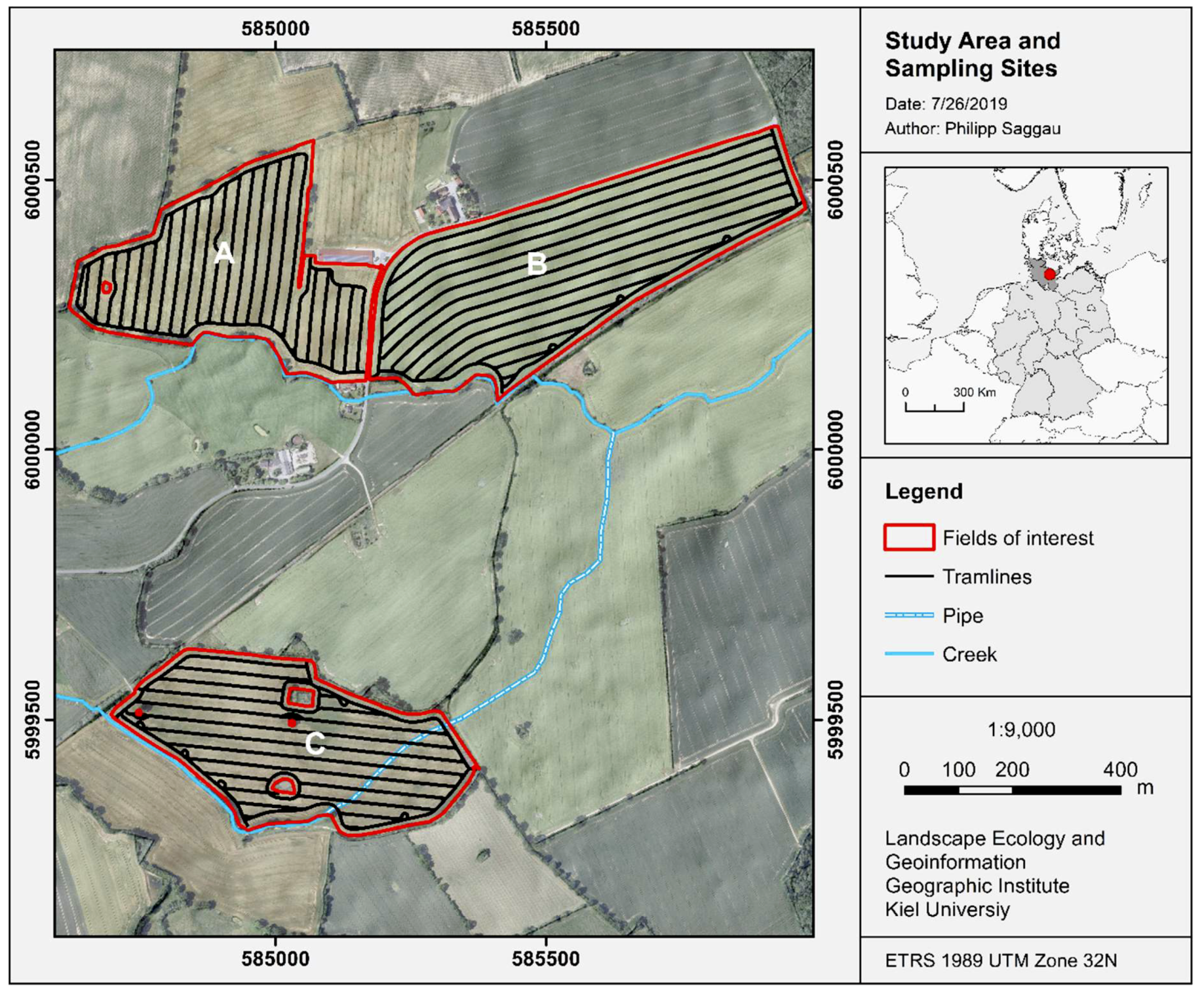
2.1. Study Area

Three fields served as study areas (Table 1, Figure 1), which were located in the Eastern Uplands of Schleswig-Holstein (Northern Germany), a landscape formed by glacial deposits of the Weichselian glaciation (54°13′ to 54°16′ N, 10°27′ to 10°32′ E). The fields belong to a catchment (5.4 km2) of the creek Mühlenbach that drains into Lake Plön. The climate is oceanic (Cfb climate of Köppen & Geiger [50]) with mild summers and winters. Mean annual temperature is 8.1 °C with mean monthly temperatures between 0.0 °C (February) and 16.5 °C (July). Mean annual precipitation is about 721 mm, although extreme years are becoming more frequent (e.g., 2017: 883 mm, 2018: 444 mm). Summer months usually receive the highest precipitation amounts followed by the late autumn months, while spring months are usually dry [51].
The parent material of the fields is deep Weichselian till from which predominantly Luvisols and stagnic Luvisols were derived [54]. Soil texture generally consists of sandy loam and loamy sand. On the steeper slopes, soils are frequently degraded forming Regosols with a more sandy texture, and colluvial deposits typically cover foot-slopes. The elevations of the fields range between 39 and 52 m above sea level with a mean slope gradient of 5.1% (range 0 to 19.6%), indicating a high susceptibility to water erosion (Table A2, Appendix A) [37,55,56].
The crop rotations for fields A and B are winter wheat (Triticum aestivum L.), winter barley (Hordeum vulgare L.), and winter rapeseed (Brassica napus L.), while field C is treated with winter rapeseed, summer wheat and winter barely (since 2016). The fields indicate uniform farming conditions, while management characteristics differ as shown in Table 1. Since the early 2000s, soil conservation methods such as the reduction of tillage intensities have been increasingly applied to these fields. Especially, mouldboard plough is regularly replaced by chisel plough. As a consequence of intensive agricultural use, all sites are drained at a depth of 1 m below surface in order to reduce the risk of compaction-induced waterlogging. The distance between the tramlines is 24 m (Figure 2) resulting in about a 6.5% share of each field, and the share decreases with increasing field size.

2.2. Model Description of EROSION 3D

Because the tramline widths can vary between a few decimeters to more than a meter, a grid-based model is needed to support the high-resolution input data. For this reason we applied the physical-based simulation model EROSION 3D (E3D) [57,58,59]. The model was chosen for several reasons: it is computer-aided, grid-based, compatible with GIS-Software, well-documented [60] and it has been validated in numerous studies and at different catchments (e.g., [24,58,61,62,63,64,65,66,67,68,69,70]). Furthermore, data requirements for E3D fit the data availability of the study area. E3D predicts soil loss and deposition for single rainfall events or sequences and consists of three components (i) the digital relief analysis (flow directions), (ii) infiltration module (runoff generation and infiltration) and (iii) the erosion module (detachment, transport and deposition of soil particles).
The relief analysis preprocesses the flow paths derived from a DEM and is used for indicating the spatial distribution of surface runoff [60]. The runoff subroutine of E3D uses the modified infiltration approach of Green and Ampt [71] to calculate rainfall excess [58]. For each grid cell, a discharge flow volume is calculated depending on rainfall intensity, infiltration rate and inflow of upper slope segments. The erosion component is based on the momentum flux approach developed by Schmidt [57,58,72]. The underlying assumption of this approach is that particle detachment is initiated, when the sum of mobilizing forces of overland flow and droplet impact (momentum flux) exceeds the soil specific forces of erosional resistance (critical momentum flux) [73]. Overviews about the model physics, its validation and the state of the art are given in many other studies (e.g., [62], [74,75,76]).
The application of E3D requires the following site-specific information: (i) relief data (DEM [m]), (ii) precipitation data (date, time and intensity [mm]) and, (iii) soil data (particle size distribution (% mass), bulk density (kg·m−3), soil organic carbon content (SOC; % by weight), initial soil water content (SWC; % volume), erosional resistance (N·m−2), hydraulic surface roughness (s·m−1/3), soil cover (% area) and skin factor (−)). Most of these variables are commonly accessible except the following model-specific parameters: skin factor, surface roughness and resistance to erosion [76]. Furthermore, bulk density is critical due to its high spatio-temporal variations in arable landscapes [63]. To facilitate the applicability of the model a detailed parameter catalogue was published, deduced from rainfall experiment simulations [77], which were extended by the results of Schindewolf & Schmidt [76]. The comprehensive database can be used in combination with the additional software tool DPROC [68,78]. It automatically assigns soil parameters as a function of land use, soil characteristics and simulation date [68,70]. E3D works on the geometric basis of a regular grid, grid size is variable, but must be consistent within the matrix. The temporal resolution of the model depends on the rainfall data availability and can range from 1 to 15 min [60].

2.3. Scenario Design

For each field we simulated two scenarios. For the Status-Quo-Scenario (SQS) we used input parameters derived according to the cultivated field section, without considering the influence of additional compaction through management operations. For the TramLine-Scenario (TLS) we differentiated soil input parameters according to the spatial occurrence of tramlines in the fields. Because E3D is grid-based, the spatial resolution (e.g., DEM, soil properties) is expected to influence the modelling results of runoff and sediment budget [79,80]. The typical spatial resolution for E3D-modelling is 5–10 m. Because tramlines are much smaller, depending on the tire width, raster cell size needs to be adapted to represent the actual spatial characteristics of the tramlines. Thus, the modelling was performed with three different resolutions (5, 1 and 0.5 m) as shown in Figure 3. The 5 m resolution was performed, as the model is well calibrated for this resolution, although its cell size exceeds the maximum outer width of the tramlines. In case of the 1 m grid size we presumed for the TLS that tramline properties are uniform between their outer widths (2.5 m), because this cell size is too large for integrating single tramlines. The 0.5 m grid size was chosen because it is smaller than the width of single tramlines. Thus, each part (left and right wheel track) could be considered separately. For soil erosion modelling, we used a rainfall event between 4th and 5th of October 2017, where measurable masses of sediments could be registered. The event that occurred lasted about 33 h with a precipitation total of 61.02 mm and a maximum intensity of about 1.55 mm/5 min.

2.4. Model Parameterization

2.4.1. Topography and Precipitation

For the application of both scenarios in E3D, we used the same relief and precipitation data. The study utilizes a DEM (airborne laser scanning method) with a resolution of 1x1 m (positional accuracy ±30 cm; altitude accuracy ±20 cm) derived from the land surveying office [81]. Following Schmidt et al. [73] we applied the FD8 algorithm for sheet flow conditions as it shows a more natural flow distribution. The rock fragment content (% mass) was considered, within the modelling process, in order to calculate the infiltration process. Meteorological data used in this study was taken from the official weather station Doernick of the German National Meteorological Service (DWD), located 2.5 km east of the study area. The precipitation data are freely available in 1-min intervals via the Open Data Server of the DWD [51]. As 1-min time steps of precipitations can indicate problems in E3D, the precipitation data was aggregated to 5-min time intervals.

2.4.2. Soil Information
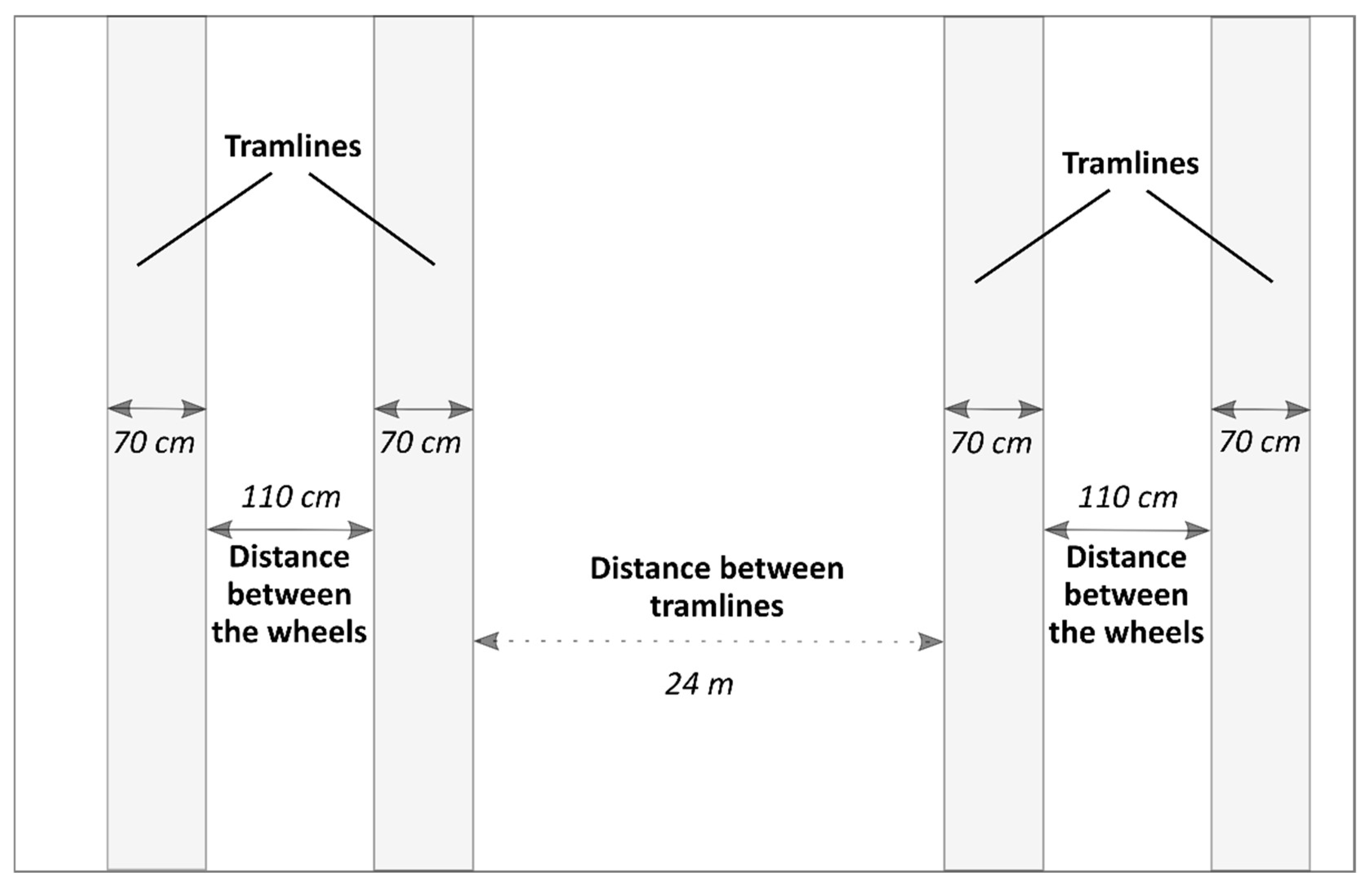
High-resolution spatial data and information about soil texture (sand, silt, clay content), rock fragments (>2 mm) and SOC were obtained from a comprehensive soil sampling of 305 points and subsequent geostatistical analysis (Saggau et al., in preparation [82]). Soil cover was derived for each field from the mean total soil cover measured at the sampling points from each field (vegetation, mulch and rock fragments). Mulch and rock fragments were estimated in the field, and photographs (RGB-camera) taken during field mapping (see below) were used to determine the degree of plant cover with ENVI (version 5.4) and supervised classification (maximum-Likelihood). Bulk density, erosion resistance, hydraulic surface roughness and skin factor, were obtained using DPROC (version 1.9), depending on the soil texture, land use, tillage practice, mulch cover and dates [83]. Because soil water content (SWC) was not measured spatially, we used the crop-model MONICA (version 2.0) to derive the spatial distribution of SWC for the investigated event. Necessary management information for DPROC and MONICA were obtained from the local landowners and farmers, who provided information about common regional crops, crop rotations, management operations, dates and fertilizer quantities. For the grid layers with resolutions of 5 and 0.5 m, we resampled the input parameters based on 1 m cell size (DEM). Resampling was performed using a decimation nearest-neighbor assignment algorithm. All raster pre- and post-processing were done with RStudio (version 1.1.4), QGIS (version 3.4.7) and ArcGIS (version 10.6.1).

2.4.3. Tramlines

UAV-imagery (Falcon 8, DJI Phantom 4; RGB-camera system) was used to derive the tramlines of the three fields by digitalization in QGIS (version 3.4.7). Afterwards the tramline data were transferred into raster according to their resolution. The rut-width was 70 cm, while the outer distance of the tramlines was 250 cm (Figure 2). In total, the area percentage varies between 6.3% for field B and 6.9% for field A (Table 1). For each corresponding tramline grid cell, we changed the parameters for cover, erosion resistance, surface roughness and bulk density based on the SQS input grids. For bulk density, we increased the raster values in the tramlines by 15% referring to suggested bulk densities of the DPROC for unwheeled areas. The assumption is following the results by Fleige and Horn [37] who found an increase of bulk density in tramlines of 15% for similar soils. The information for erosion resistance and hydraulic surface roughness were derived directly from the parameter catalogue by Michael et al. [77], which suggests specific values for tramlines, given management conditions and soil texture. Finally, soil cover was limited to the cover of rock fragments and mulch since no plant cover existed in the tramlines (Table A2, Appendix A).

2.4.4. Field Mapping

Soil erosion and soil cover by vegetation, mulch and rock fragments were mapped on the fields directly after the rainfall event considered in this study. The mapping method focused on the quantification of soil loss by linear erosion. Sheet erosion was documented by its location but not taken into account for soil loss calculations, because that amount of soil loss cannot be quantified by exact measurement. The erosion mapping was based on a method given by Rohr et al. [84] and DVWK [85]. We measured the lengths and the cross-sectional areas on representative morphological positions of linear erosion features (rills, ephemeral gullies), with a folding yardstick. The incision volume was calculated for each section and the mass of eroded soils were calculated by multiplying volumes with measured average topsoil bulk densities [86]. A more detailed description is given by Ledermann et al. [87]. In contrast to the mapping approach suggested by Steinhoff et al. [88] we located erosion structures with dGPS (Leica Viva CS 10, GNSS GS08 plus), which assured high spatial accuracy for validation (<5 cm). To calculate the soil loss rates from rills in t·ha−1, all linear segments of each field are summed and related to the field size.

3. Results

The following paragraphs give a detailed description of the 1 m resolution modelling comparing SQS and TLS. Afterwards, the effects of different spatial resolutions (5 m and 0.5 m) are demonstrated, followed by an evaluation with the mapped soil erosion.

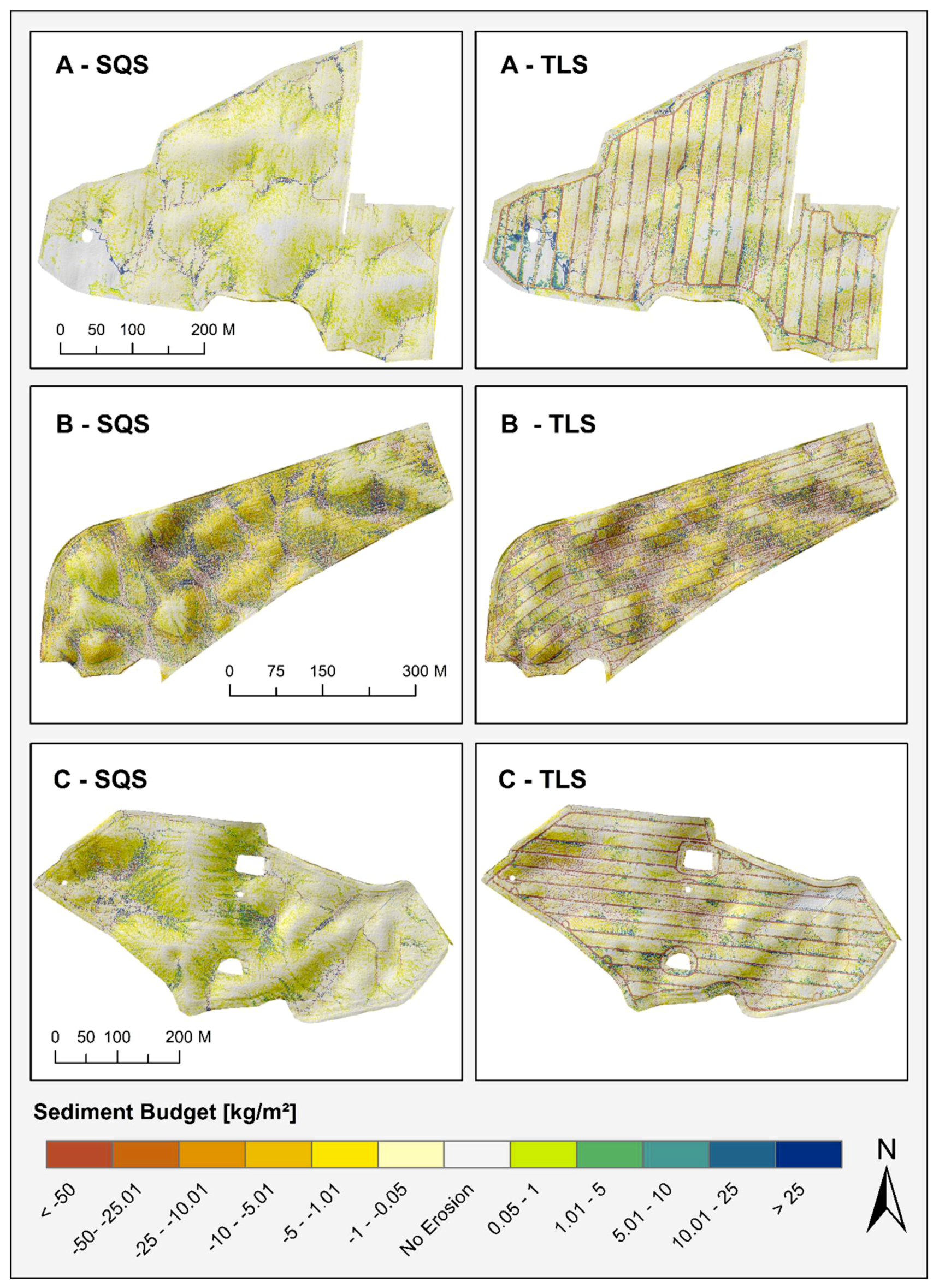
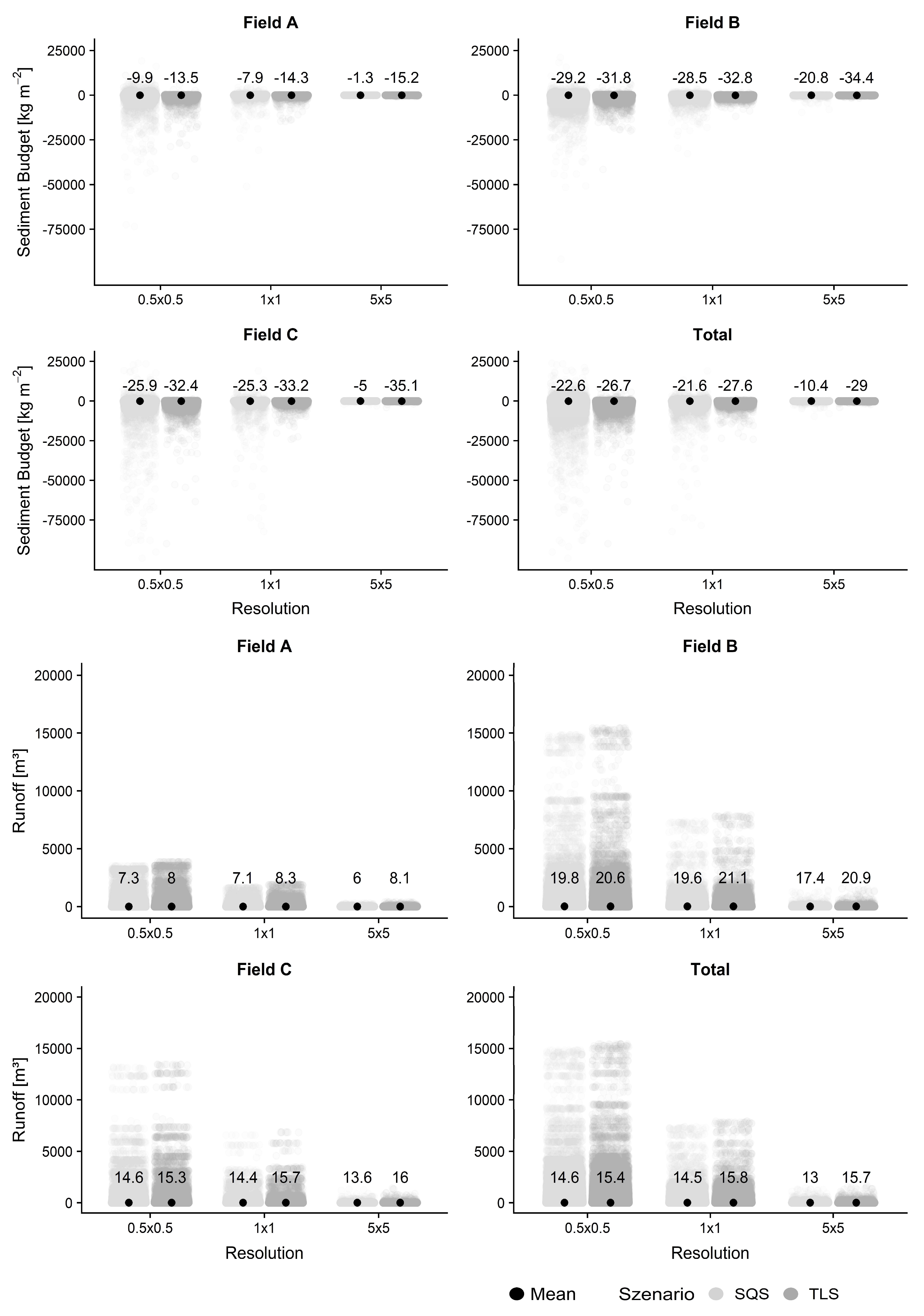
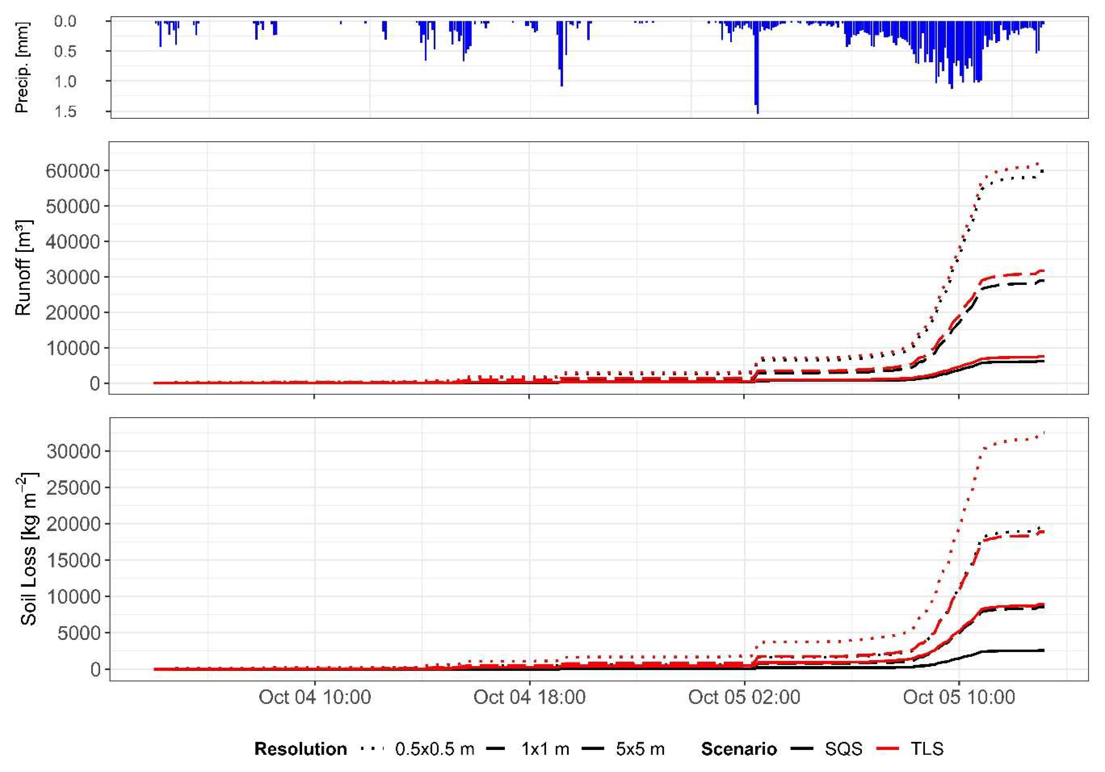
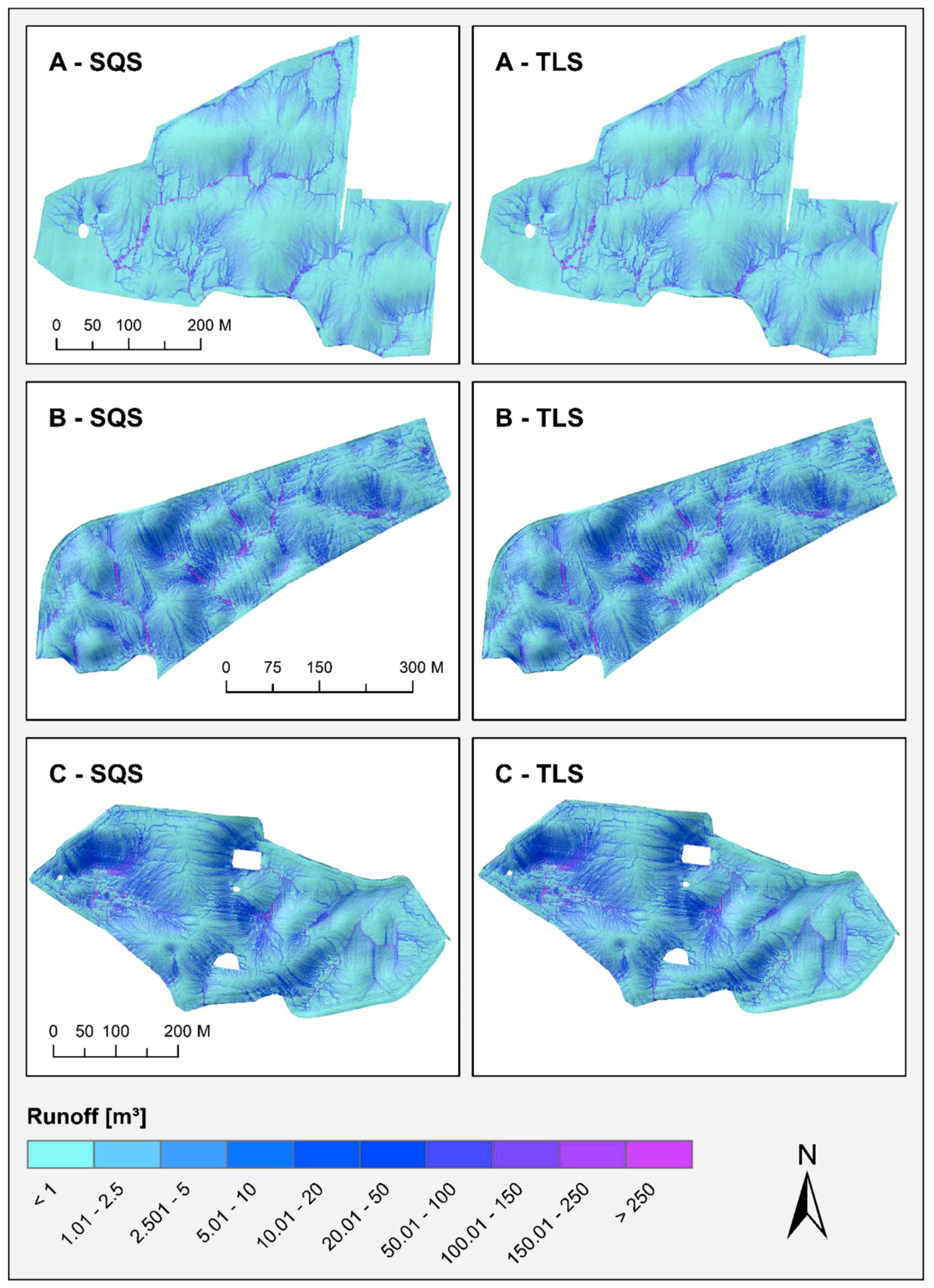
3.1. Modelling Results

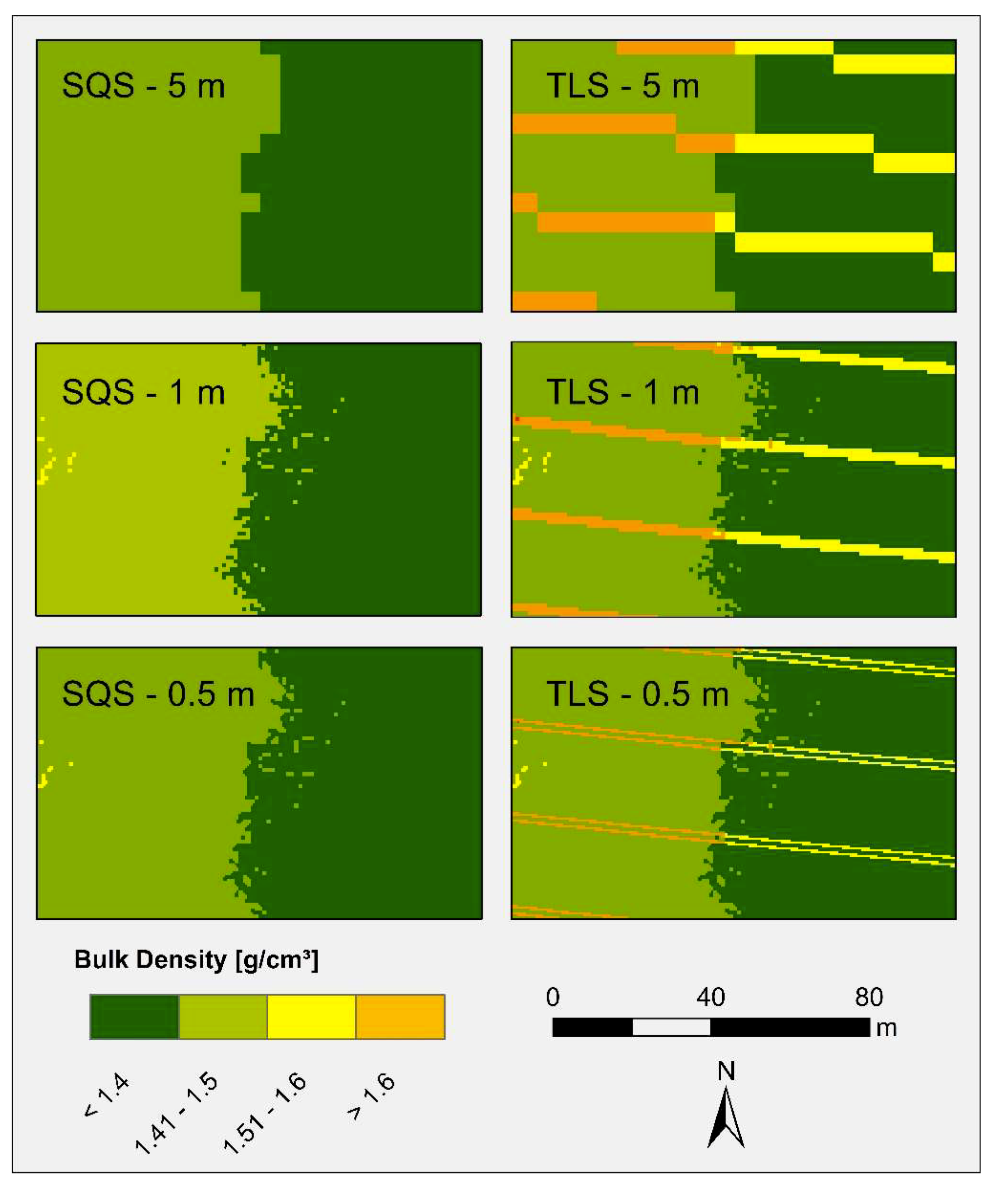
3.1.1. Status-Quo-Scenario (SQS)

The sediment budget delivered by E3D shows a diverse distribution of erosion and deposition patterns over the fields. Comprising all three fields, the sediment budget for the simulated event yield in high mean soil loss rates of 21.6 kg m−2 (216 t ha−1), which equals 10,237.7 t of total soil loss. Nearly half of the cells (49%) affected neither by erosion nor by deposition (gray areas in Figure 4).
Soil loss occurred at 40% of the total area (<−0.05 kg m−2), while alluvial deposits cover 11% (>0.05 kg m−2). The model results indicate that cells of high deposition values are limited to level areas in concave relief forms. Furthermore, cells of high deposition and high erosion rates (> ± 10 kg m−2) are dense were runoff is channeled. For all fields 6.9 mil. M3 runoff were shifted across the cells, which are in average 14.5 m3 per cell. The maximum of total runoff was found at the outlet of field B with 7381.8 m3. However, most of the areas that are located on more gentle slopes show values of<1 m3 (Figure A1, Appendix A).
Focusing on the individual fields, the highest soil loss and runoff amounts were detected for field B with an average soil loss of 28.4 ± 314.5 kg m−2, which contributes to 54.5% of total soil mass moved over the surface. On this field soil loss affected 42% of the area (ca. 8.3 ha). The runoff simulation shows the highest mean of 19.6 ± 187.9 m3 for field B. In contrast, field A shows lowest soil loss rates with a mean of 7.9 ± 278.2 kg m−2 which is about a quarter of the soil loss of field B and 36% less than the average. Although the distribution of areas affected by soil loss is similar to field B the magnitude of their loss rate is much less. Runoff generation is relative poor for that field with 7.1 ± 65.7 m3. Field C reveals the second-most soil loss with 25.3 ± 792 kg m−2, which is close to the total average. This field experienced, the highest deposition 18,975 kg m−2 (Max) and highest soil loss rates −106,637 kg m−2 (Min), indicating high differences in the erosional distribution. The strong scattering of cell values is also confirmed by the high standard deviation. Besides the high soil erosion rates, field C shows the highest aerial share of deposition with about 17%, which is quite higher than for field A (13%) and field B (12%). The high spatial distribution of depositional areas at field C is also noticeable in contrast to the other fields. Table 2 shows for the 1 m grid size that high standard deviations and distribution of maxima and minima indicate that runoff and sediment budget of the model results are scattering strongly.

3.1.2. Tramline-Scenario (TLS)
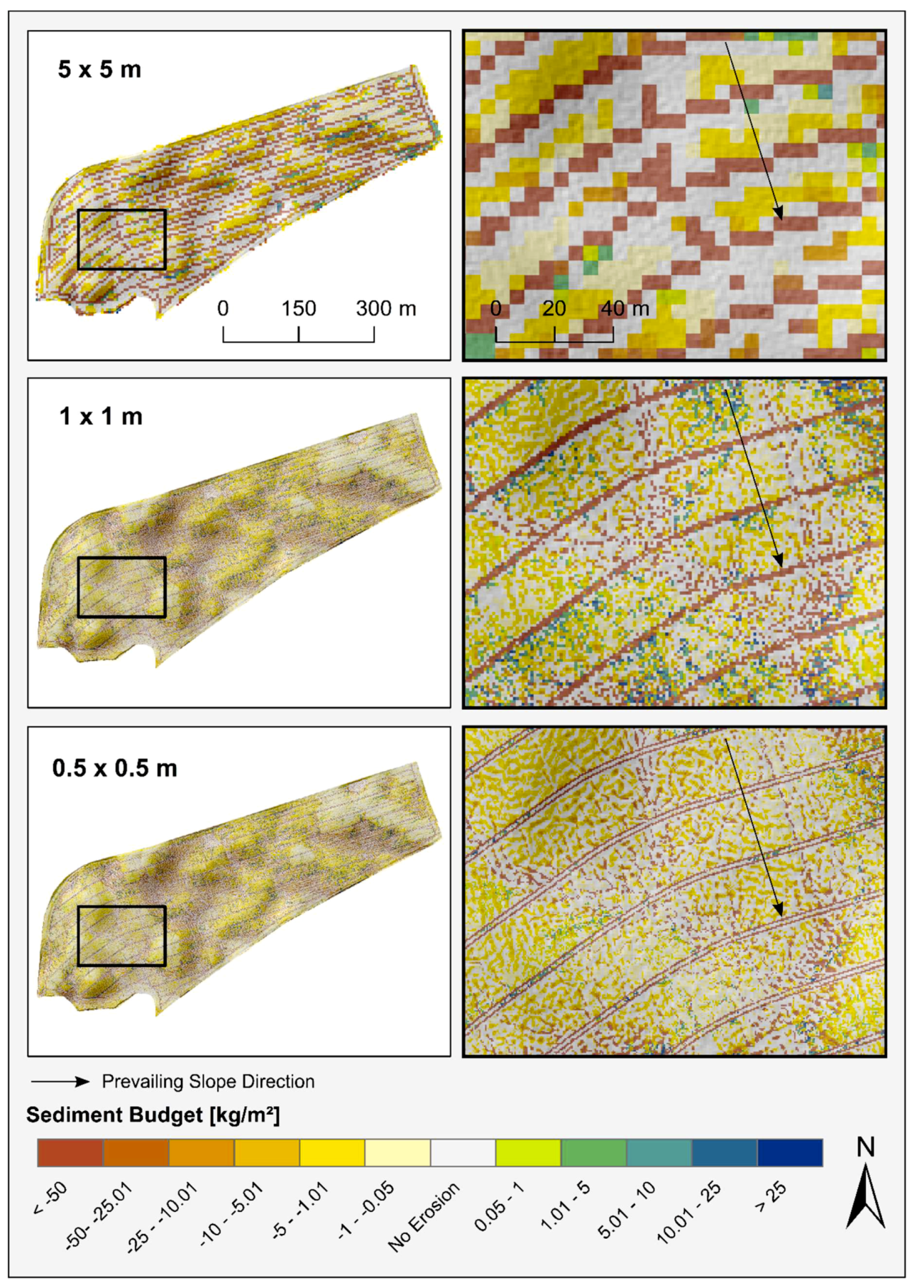
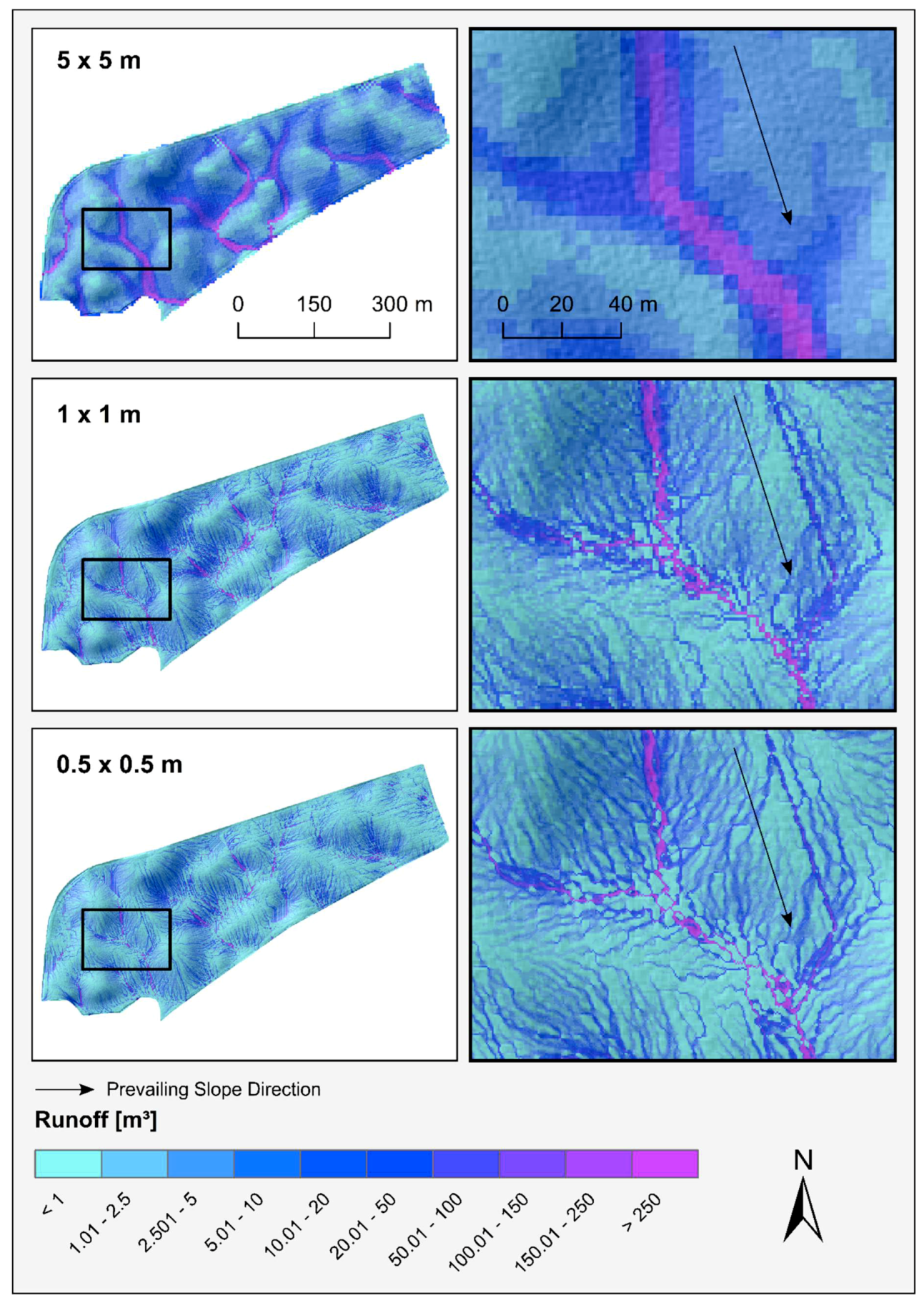
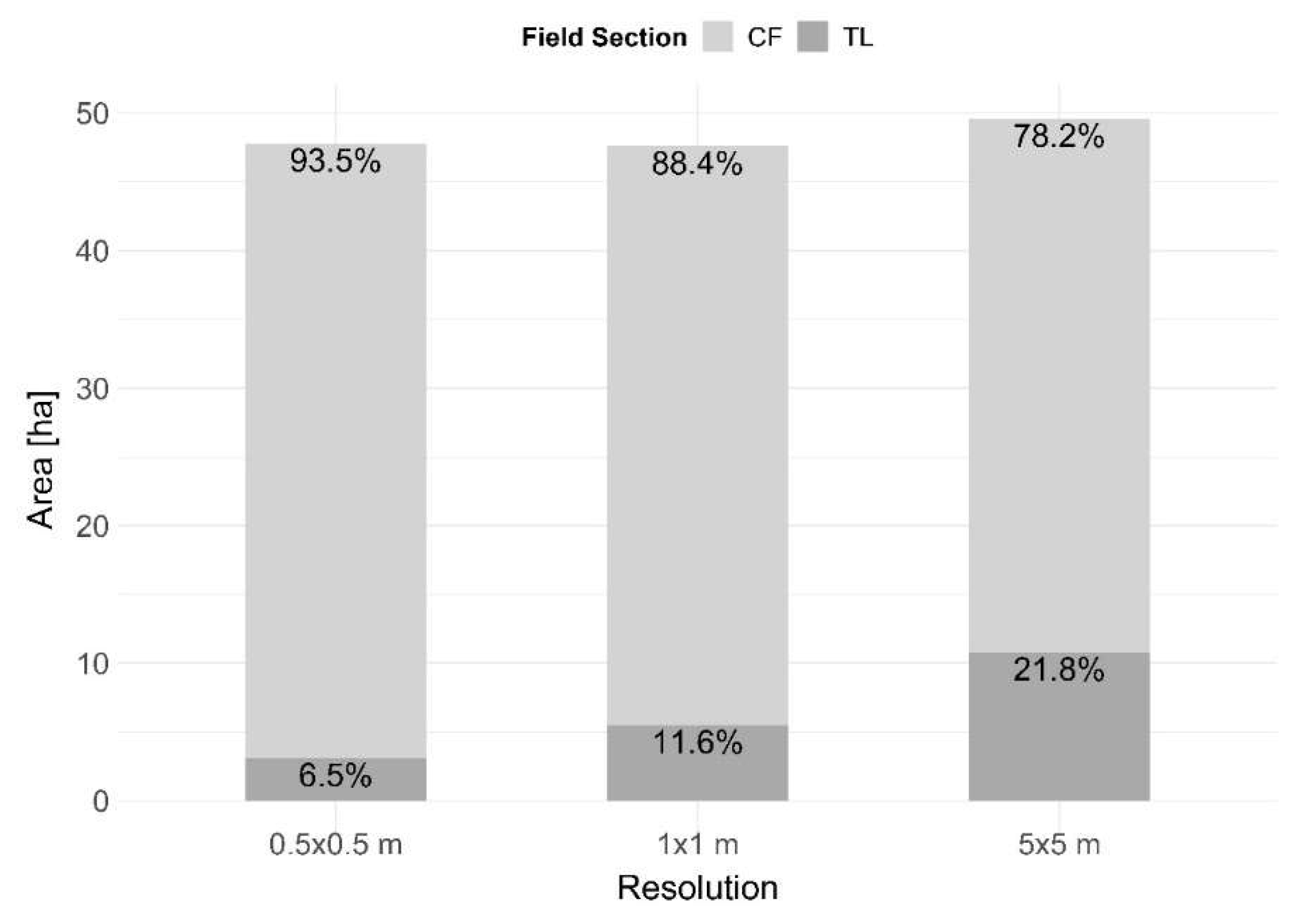
According to the sediment budget results, the area where soil loss occurs is increased by 3% in contrast to the SQS, while the area of deposition decreased by 2%. The increase is mainly attributed to field B, where erosional areas increased from 42% to 52%. In contrast, fields A and C exhibit decreased areas affected by soil loss and deposition.
The spatial adaption of central input parameters for tramlines resulted in an 8% increase of runoff (15.8 m3) and soil loss of 21.7% (Figure 5, Table 2).
Mean soil loss for field B increased less from 28.5 to 32.8 ± 163.8 kg m−2, while field C exceeded soil loss rates of field B to 33.2 ± 283.2 kg m−2 (25.3%). For field A, soil loss rates were nearly doubled to 14.3 kg m−2 (44.8%). In total, the scatter increased but more strongly for fields A and C (Table 2). Figure 4 shows that the soil erosion distribution for the TLS shifted to a continuous soil detachment in the tramline sections for all fields throughout the rainfall event. Additionally, the spatial integration of tramline properties leads to an increased runoff generation (Figure 5, Table 2). The relative highest gain of runoff for the TLS was observed for field A (14.5%) followed by field C (8.3%) and field B (7.2%), which reflects the trend for soil loss.
Output parameters (runoff, sediment budget, etc.) were calculated as a sum of the major outlets of each field for each time step of the precipitation event (5 min). Figure 6 shows the temporal generation of runoff and soil loss dynamics. The Figure also indicates that both parameters strongly increased at 2 a.m. of 5th October when the highest rainfall intensities of 1.5 mm per 5 min were measured. Runoff and soil loss were initiated more rapidly and increased stronger for the TLS, which results in an increased discrepancy in comparison to the SQS.
Table 3 shows the sediment budget and runoff comparing the tramline zones with the cultivated field sections. Total soil loss rates in tramlines are about one magnitude higher compared to the cultivated field and account for half (50.2%) of the total erosion on all fields. In contrast, runoff stays nearly the same for both areal sections with similar standard deviations. Differences between the individual fields are high. Simulations for field A indicated that 78.3% of total erosion took place in tramlines, which represent 11% of the field. Trends of soil loss at field C are similar; 60.4% of the total erosion are triggered in the tramlines with the highest soil loss rates of 162.7 ± 599.1 kg m−2. Additionally, field Cshows 22.4% higher runoff in tramlines compared to cultivated areas. Field B is the only field with higher soil loss rates in the cultivated field section. Tramline erosion takes about a third (34.1%) of total soil loss here. The relative small share can be explained by a high mean of −24.3 ± 145.9 kg m−2 in the cultivated section, which is eight times the amount of field A (−3.5 ± 84. 7 kg m−2).

3.1.3. Resolution

The results for the different spatial resolutions (0.5 and 5 m) indicated an increase of runoff and soil loss with higher spatial accuracy (decreasing grid size) in terms of SQS, and far more scattering values (Figure 5). While the amount of runoff from 5 m grid to 1 m increased by 10.3%, the increase from 1 to 0.5 was much less with 0.7%. This is noticeable for all fields. For soil loss, the trend for the SQS is the same, although the increase is higher. While soil loss is doubled (51.9%) from 5 m to 1 m grid size it increased by 4.4% from 1 to 0.5 m resolution. In contrast, the TLS shows a slight reduction of soil loss with increasing spatial accuracy.
For all fields the decrease of average soil loss from 5 to 0.5 m is as follows −29.0 > −27.5 > −26.7 kg m−2. For runoff, no clear trend between single fields can be identified. While field C showed a decreasing runoff with increasing resolution, A and B showed an increase from 5 m to 1m followed by a decrease from 1 to 0.5 m resolution. The inverse trend of the TLS in comparison to SQS can be attributed to the more accurate representation of tramlines with finer resolution (Figure A2 and Figure A3, Appendix A). This implies a smaller area share of tramline properties in scenario modelling (Figure 7). For the 0.5 grid size, tramline areas (3.12 ha) are spatially well presented in comparison to the real tramline areas mapped (3.15 ha), which show an accuracy of 99%. Resolutions of 1 and 5 m increasingly overestimate the tramline area by exceeding their spatial extent. This effect is also indicated in the temporal resolution from Figure 6 were the discrepancy of soil loss for TLS and SQS are getting even stronger with decreasing cell size. Unlike the soil loss, runoff increases more evenly with decreasing grid size, although the total amount of cumulative runoff shows a clear increase at the outlet.

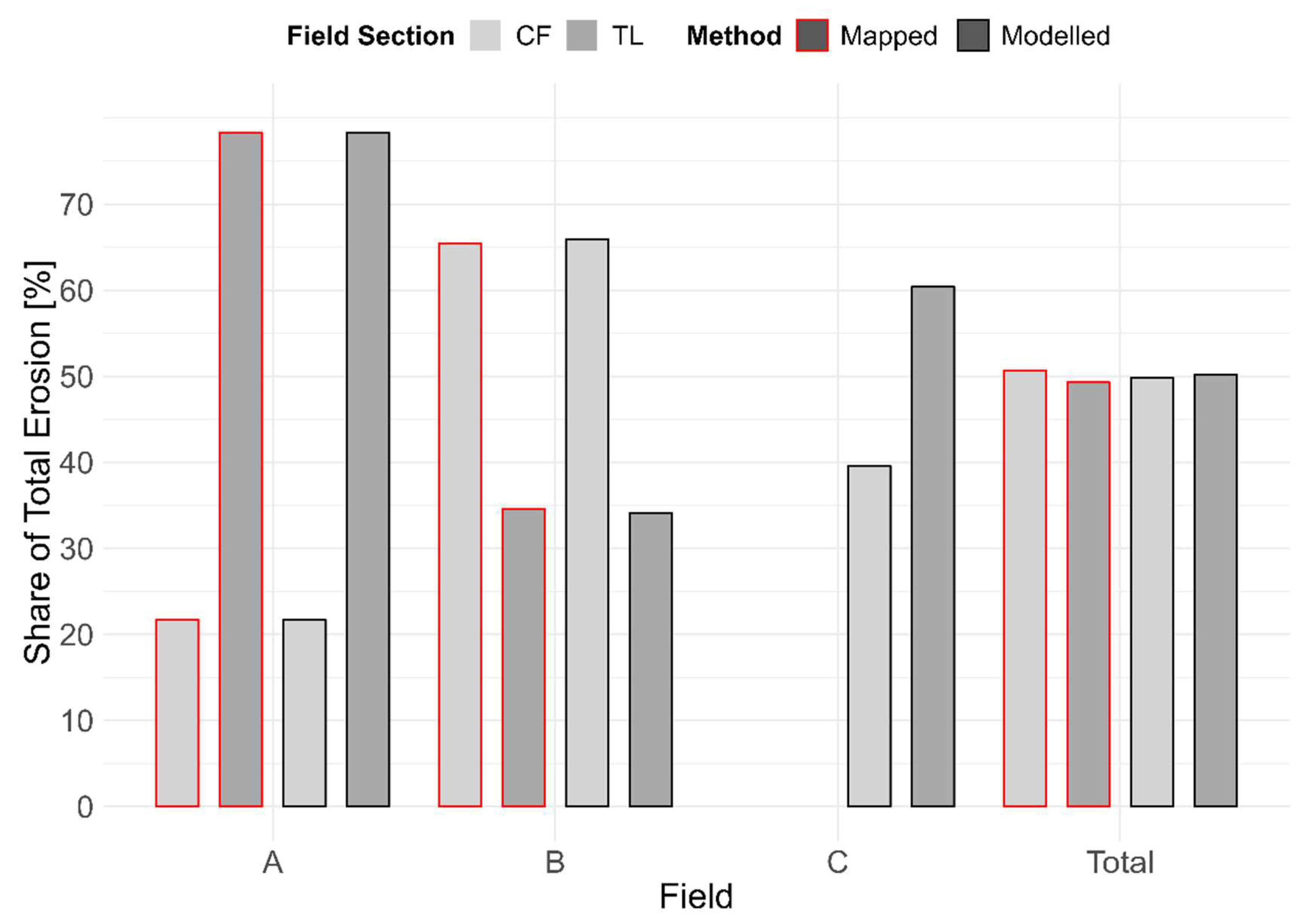
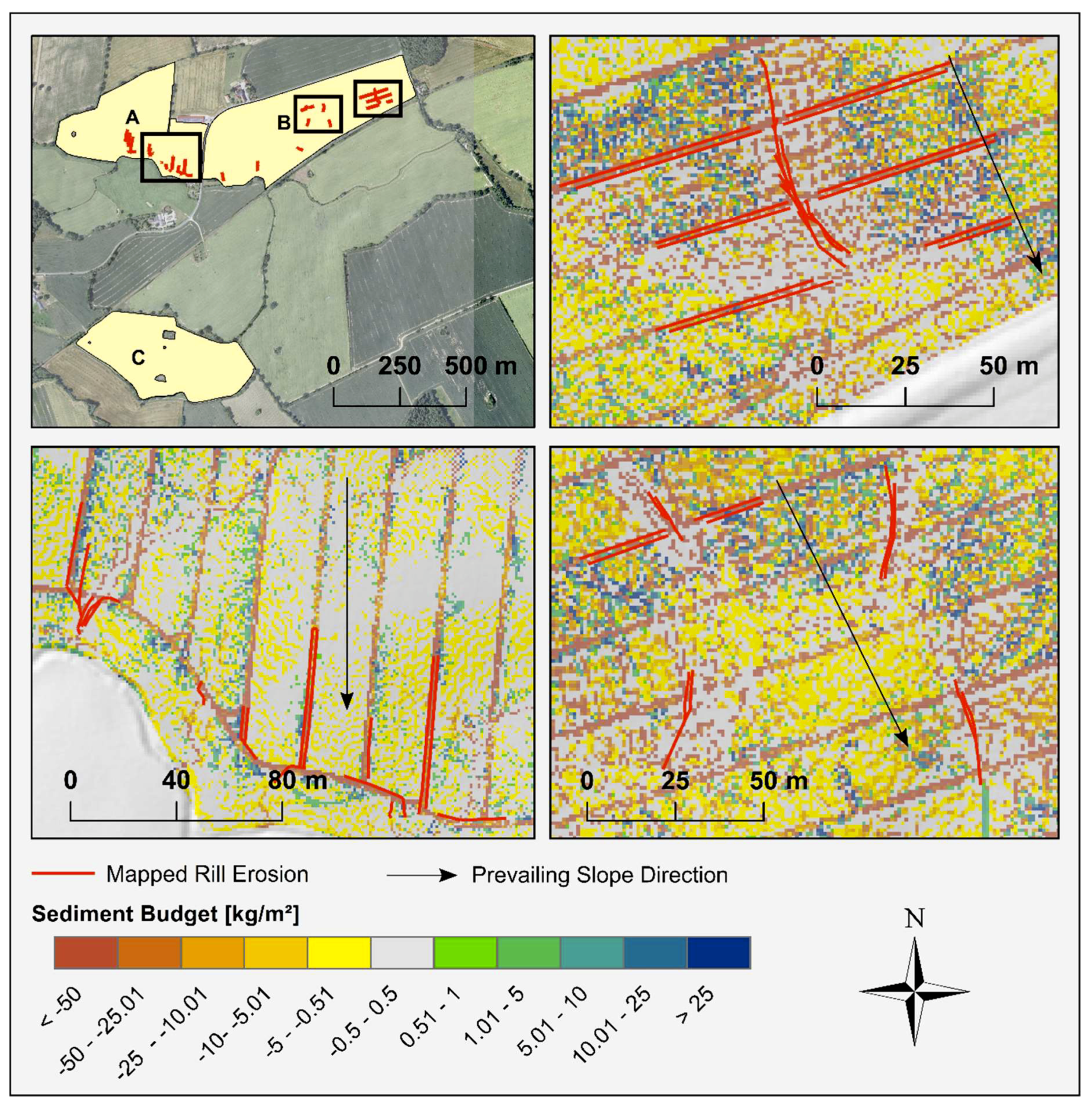
3.1.4. Mapped Soil Erosion

Soil erosion mapping after the rainfall event in October revealed soil losses in form of sheet erosion on all three fields. Especially rinsing could be found in all tramlines, with varying degree of intensity depending on slope. On level slopes at higher elevations, the ruts showed rinsing in the middle of the ruts, while on steep slopes ruts were totally washed away. At the foot—slopes of tramlines, high amounts of depositions were observed. However, the absolute masses of those accumulations were not measured and thus were not available for this study. Sheet erosion on cultivated areas was observed on nearly all slope segments, however with lower intensities compared to tramlines.
Rill erosion was only found on fields A and B (Figure 8), while field C showed no definite rill erosion structures. Rill erosion mapped reached highest amounts on field B with 29.2 t of soil material (1.5 t ha−1), which was found on an area of 402.3 m². Furthermore, we found 1148.1 m of rills on eight different hot spots on field B. According to Figure 9 about a 34.6% of the mass eroded by rills were found in tramlines, while 65.4% occurred in the field in concave major flow pathways. In contrast, in field A 78.3% of the rills occurred in the tramlines, which is four times more than in the cultivated area. In total, fewer rills were found for field A with a total length of 772 m and a total amount of 14.8 t (1.1 t ha−1).

4. Discussion

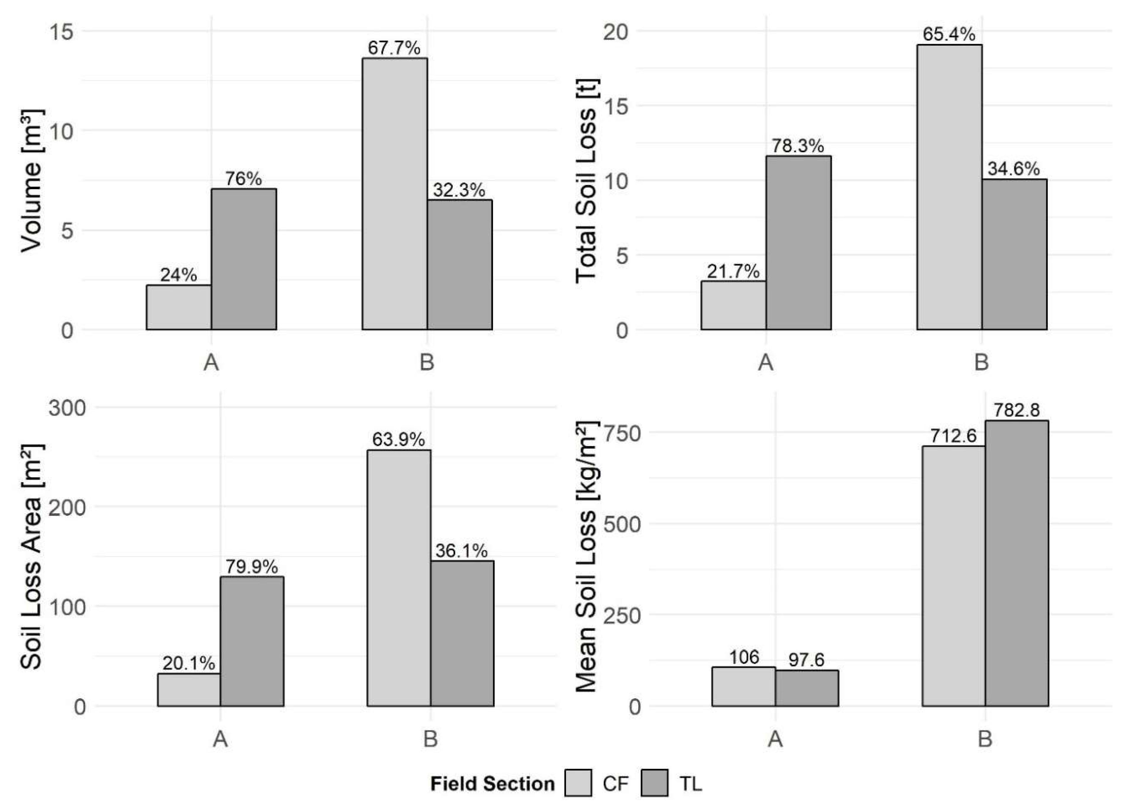
4.1. Effects of Tramlines on Runoff and Sediment Budget

This study demonstrated the effects of tramline integration on soil erosion modelling. Through an adaptation of input parameters at areas of tramlines (surface roughness, soil erosion resistance, vegetation cover and bulk density), a higher and faster generation of runoff and soil loss occurred over time. The higher amount and speed of simulated runoff as a result of inhibited infiltration paired with lower soil resistance contributed to higher soil loss rates in the tramlines. Furthermore, the spatial pattern and distribution of soil erosion and depositions changed significantly between SQS and TLS. Soil erosion mainly occurred in tramlines, while deposition was often found close to them due to gains in runoff and therefore a higher transport capacity of soil particles. Thus, the integration of tramlines into soil erosion modelling reflects the findings of several field studies involving the influence of soil compaction on soil erosion (e.g., [37,89,90]).
The modelled amounts of soil erosion, deposition and runoff, however, were relatively high for both scenarios (SQS and TLS). Possible reasons for this are discussed in the following section (4.2), as it may depend on model performance. Despite the absolute amounts of soil loss and deposition, the shares of soil erosion within tramlines agree with the findings of other studies. For instance, Fleige and Horn [37] measured soil loss on similar soils for the growing season 1996/97, which was in average 79 to 84% higher compared to unwheeled field sections. However, our investigations show that erosion in tramlines averages 89% higher, but depending on the field characteristics ranges between 80% (field B) to 97% (field A). Although the results of the study by Fleige and Horn [37] fit quite well for field B, fields A and C indicate that soil loss from tramlines make a higher share of the total erosion than has previously been reported. The higher share might be attributed to the orientation of tramlines to major slopes. While tramlines are predominantly oriented parallel to contour lines for field B, tramlines of fields A and C are orthogonal to the slope. This means that for fields A and C runoff is more channelized in tramlines, which leads to a stronger increase in erosion and runoff. Contrary, at field B, channeling effects caused by tramlines are disrupted with cultivated field areas (Figure A1), which according to model outputs are characterized by higher infiltration rates.
The direction of tramlines seems to have a strong influence within the modelling process as soil loss is more strongly increased for fields A and C compared to the model results of the SQS. This is also confirmed by the overall maximum soil loss of field C, which was located at the end of a tramline with an extremely long slope length (220 m). In contrast, the erosion−prone field B showed a low increase for TLS (Table 2). Surprisingly, no significant differences were found in runoff generation among tramlines. While in total TLS results showed an increase in runoff, of 7 to 14.5%, the average increase within tramline areas was only 0.5% higher and on field A (−2.5%) and B (−3.3%) even lower. This is surprisingly, as compacted soils in general show much higher flow velocities and Fleige and Horn [37] reported from experiments that runoff in tramlines is usually increased by 3.8 to 5.3 times compared to unwheeled areas of the field. As a consequence, the model response to runoff generation in tramlines seems to be poor.
We assume that this aspect might be an issue of the input DEM. Our measurements found that tramlines average about 6 cm deeper compared to surrounding surface which is confirmed by other studies [35,37]. However, in our modelling approach, we have used a 1 × 1 m DEM that precludes the consideration of micro—relief at this scale. This might also be a reason why depositional areas were simulated close, but outside of tramlines, and why the model could not reproduce our findings of mapped soil deposition in the sinks of tramlines. A burning of tramline depth into the DEM could optimize the reproduction of preferential overland flow and sediment transport. This kind of parameterization might also be improved with UAV and structure from motion techniques, which are able to derive DEMs with a resolution and accuracy of 0.2 cm, and could incorporate tramline depth directly. However, such high spatial resolution would greatly increase the calculation time (see Section 4.2).

4.2. Model Performance

4.2.1. Modelled vs. Mapped Soil Erosion

Primarily, the comparison of mapped erosion with model results of E3D showed that model outputs were plausible in terms of the areal distributions of erosion and runoff. According to Figure 4, the highest soil loss rates are linked to major flow pathways with concave relief forms, which match well with our observations. The TLS performed with much better results than SQS as it could account for erosional hot spots in tramlines, which were also detected by field mapping. Furthermore, the shares of simulated erosion in tramlines compared to erosion in the field were well represented in the mapping results. Additionally, our mapping confirmed the findings from model prediction, as field B is much more erosion−prone than field A. For field C it was difficult to draw conclusions from the mapping because no rills could be measured.
Regarding the model performance between erosion inside and outside of tramlines, the modelled share for field B is lower in the tramlines than in the cultivated field, which fits the measurements of mapped rill erosion. Fields A and C, however, have a higher share of soil erosion in tramlines than in the field, which in case of field A also fits the occurrence of measured rill erosion (Figure 10).
One unanticipated finding was that simulated soil erosion rates in tramlines in general were relatively high in contrast to soil loss from cultivated fields. Our findings of rill erosion in tramlines, in comparison to model results, however, were very poor. The highest amounts of rill erosion were estimated by E3D in field C, where no rills could be found during field mapping. The explanation for this might be that compacted soils are generally more resistant to rill erosion compared to soils with looser soil material. This is because soil shear strength increases with increasing bulk density and tends to retard rill erosion [91]. Hence, it could be hypothesized that for the rainfall event more soil loss in tramlines is initiated by sheet erosion than in unconsolidated areas of the fields. However, yet there are still gaps in our understanding of the factors and mechanisms that affect sheet and rill erosion rates [3]. Another possible explanation for the high—simulated soil loss amounts in tramlines is the parameterization of input parameters. Although we used reasonable values for surface roughness, bulk density and erosion resistance, those parameters are unfortunately very sensitive in E3D [61]. The occurrence of local variability among rainfall intensities for that event could also be a reason for differences between mapping and modelling. This is confirmed by radar precipitation data gathered for the research area that indicate a scattering of rainfall intensities for the investigated time. Additionally as field C was covered by stubble fallow and managed with chisel ploughing soil conditions might have indicated a higher resistance to soil erosion than suggested by the DPROC (e.g., soil erodibility, skin factor, surface roughness, bulk density) due to limitations of the database for such particular combinations. In this case, soil erosion resistance and infiltration rate would have been higher for field C, which might have prevented rill formation.
When comparing measured and simulated sediment yield (Section 3.1.2 and Section 3.1.4) it becomes evident that the results of E3D overestimate real erosion rates about two magnitudes for 1 m resolution. Although we followed the findings by Bug [36] who estimated that rill erosion accounts for an average 25% of total erosion, our modelled soil loss exceeds our mapped findings by far. The share of rill erosion on total erosion however is a subject of debate and might vary between 10–99% depending on slope steepness and climate [92,93,94].
It must also be stated that soil erosion mapping is frequently error prone. Error rates in the methods applied for quantifying linear erosion might range between 15–30%, depending on the experience of the observer [12,86]. Therefore, further research should be undertaken to investigate other methods, which could account for sheet erosion and identify rill erosion easily with reduced error. Here UAV might fill the gap [62,95,96]. Erosion and runoff modelling, however, is also error prone [61]. E3D, for example, tends to overestimate results when used uncalibrated, which has been confirmed by other studies [69]. Errors in the model outputs could be caused by deficits in model design especially with respect to channel processes, which are not represented in the model by specific algorithms [62]. Furthermore, generalized input data taken from the DPROC or the E3D parameter catalogue may not represent conditions for our study area very well. Spatial error propagation is postulated to be more of an issue in catchment−scale models than it is in field—scale models [61]. In order to improve the model results in terms of input parameters additional calibration is necessary.

4.2.2. Effects of Cell Size

According to our findings based on predictions at different spatial resolutions, a higher spatial accuracy of tramlines with smaller grid size could be achieved (99% accuracy for 0.5 m grid). However, no strong improvements could be made in terms of quantification of soil loss. The 5 m grid resolution for the SQS can be regarded to perform best in terms of quantities. However, assuming that the mapped rill erosion made 25% of total soil loss (in accordance to Bug [36]), the SQS results for the 5 m resolution are still overestimated by about one magnitudes (373%). Thus, E3D performs generally well with 5 m resolution for SQS, however, the integration of spatial overestimated tramlines for TLS leads to an unsatisfactory overestimation of the soil loss amount by two magnitudes (1035%). In contrast, the results for total erosion of 0.5 and 1 m scenarios are very similar and in terms of SQS about twice as much as for the 5 m resolution. In comparison, for TLS, model results improve slightly with finer resolution. In addition, finer resolutions improve the optical representation of the results. Furthermore, the share of tramline erosion compared to cultivated field erosion is reproduced by measured soil loss for 1 m and 0.5 cell sizes.
According to these findings, we suggest that the adaptation of resolution for the spatial integration of tramlines should usually be favorable as areal relations can be reflected and distinct relief forms can be regarded more properly (tramline depth). This approach is especially important in areas were relief forms can change rapidly. Consequently, we conclude that the field−based integration of tramlines should employ resolution of 1 m or higher. However, a calibration of our approach must be tested. An uncalibrated use of E3D, which regards tramlines, still helps to improve spatial occurrence of runoff and soil loss. A decision must be made about whether the required time and processing efforts justify improvements that can be obtained from this approach. The processing for 0.5 m was very time intensive (several days) while results for the 5 m resolution were produced in a few minutes. A “good practice approach” for uncalibrated use of E3D and tramline integration might be a hybrid approach. For example, results can primarily be simulated without tramlines using 5 m resolution as the SQS, which can be processed quickly and showed rather satisfactory results in terms of soil loss rates. A second simulation, to integrate tramlines on a 1 m grid size, can account for spatial occurrence, share, and the effect of the direction of tramlines.

4.3. Future Work in Soil Erosion Modelling

In general, several aspects can improve the outputs of future modelling. The first one concerns the effect of sealing (or crusting) in tramlines. Sealing decreases infiltration rates and therefore increasing runoff [22], due to the formation of an underlying platy soil structure [97,98,99]. The sealing effect can be adopted by changing the skin factor. Furthermore, the spatial distribution of soil water content might be improved with a soil moisture model that takes into account the effects of relief and lateral water movements. This might be important as ‘initial soil moisture’ is a sensitive parameter in E3D [70]. Further, it can be assumed that initial water contents vary in tramlines. In our study we used values derived from uncompacted field areas, however, compacted soils frequently show reduced soil water contents. The use of pedotransfer functions (e.g., by van Genuchten) may enable the adaptation of soil water content for the compacted areas in the tramlines. In addition, spatial variation of plant cover should be considered more accurately in field−based modelling. The mapped soil cover inside the field was highly variable and ranged about ±20%. An adaption of these parameters might draw a better picture of the underlying process and should be a point of further investigation.
As we estimated results on the field scale, we could not measure and compare runoff characteristics for model outputs. Therefore, a catchment−based approach is needed. This would be also valuable as on the catchment scale the contribution to sediments and pesticides from tramlines to adjacent surface waters and ecosystems can be determined [60,61]. Sediment yield data for catchments are crucial for better understanding the linkages between soil erosion processes and sediment transport in large rivers [3,100,101]. We derive from our findings that the integration of tramlines should also be possible for other grid—based erosion models as long as required input parameters are known or available. In this context, helpful tools like DPROC in case of E3D should be extended further. This could facilitate the application of tramlines for such models and help with resolution issues.
As our investigation focused on soil erosion characteristics of a single erosive event, the results have not addressed broader scales, which are valuable in terms of annual rates. Tramlines in particular, are not only affected during such erosive events, but also affected frequently during the season, as they do not support a closed plant cover. This will require research studies that focus on a continuous modelling approach for an entire growing season. Continuous simulations could take into account the variability of input parameters throughout the year, however, they can consider the share of soil erosion and runoff for multiple events and cover broader time scales. Accordingly, long—term simulations of sediment yields over several years should draw a more accurate picture of the temporal occurrence of soil erosion than compared to those for single events [102]. Most of process—based soil erosion models have capable options for these kinds of simulations.
Our findings suggest that incorporating tramlines in soil erosion modelling facilitates the base for evaluating and adapting proper conservation measures. For example, the effects of tramline operations to the field slope can be assessed. Scenarios with different tramline angles can be modelled and soil risk can be weighed against operating costs. This is also true for the integration of intermittent or total planting in tramlines. Several studies showed that these measures can reduce soil loss by 25–80% inside the tramlines [103,104]. Those management practices could easily be integrated in scenario—based modelling. Furthermore, areas of compaction in arable lands are not limited to tramlines. They occur in all kinds of wheel tracks initiated from harvesting, cultivation and other agricultural activities. The headlands of a field are especially problematic because they exhibit the highest field traffic intensity (e.g., Duttmann et al. [47]). Thus, a further challenge for future modelling will be to identify those areas (e.g., by the SaSCiA model developed by Kuhwald et al. [105]) and integrate them in the model process.

5. Conclusions

In this study, the application of a process−based soil erosion model, which considers field−based compaction effects of tramlines, was successfully performed for the first time. In detail, our study revealed that:
  • Grid−based erosion models like E3D are able to integrate tramlines.
  • The share of measured soil loss between tramlines and cultivated areas is well accounted for on grid sizes ≤1 m.
  • The integration of tramlines showed a high dependency to the angle of slope. Therfore, the increase in estimated soil loss was higher for fields where tramlines were in the direction of the major slope, as confirmed by mapped soil erosion.
  • The soil loss and runoff were initiated quicker and increased stronger within tramlines.
Although the amounts of soil loss and runoff were overestimated, the integration of tramlines in soil erosion modelling revealed a more accurate distribution of soil loss over the land surface, which was confirmed by field mapping. Based on these results we conclude that tramlines should be included in similar soil erosion modelling studies in order to generate more realistic soil erosion and deposition patterns at the field−scale. However, to confirm our findings and to expand our knowledge of tramline integration in soil erosion modelling, more research is needed. We suggest that further research could focus on calibrating finer spatial resolutions (e.g., catchment−scale), long−term simulations, and improving the parameterizations of such models. Despite the limitations mentioned above, this study is a step forward in the application of process−based soil erosion models at the field−scale. The implications of this study could help soil conservationists, advise planning authorities and guide farmers towards a more comprehensive use of detailed erosion control measures.

Author Contributions

Conceptualization, P.S. and M.K.; Data curation, P.S. and M.K.; Investigation, P.S.; Methodology P.S. and M.K.; Software, P.S. and M.K.; Validation, P.S.; Writing—original draft, P.S.; Writing—review & editing, P.S., M.K. and R.D.; Supervision, R.D.

Funding

This research was supported by the Federal Ministry of Education and Research within the framework of the BonaRes (grant number: 031B0684C).

Acknowledgments

First we like to sepcial thank the landowners and farmers of the study area who freely provided sensible but valuable informations for the study and made their lands accessable for investigation. Thanks also go to the anonymous reviewers for their valuable and helpful comments, on improving the article. We thank M. van Werner for technical support with EROSION 3D and of course all our lab members for contrbutions. We are grateful to James F. Petersen for linguistic editing. Finally we thank A. Berger, M. Gosse and J. Goldmann for comprehensive assistance in the lab analyses.

Conflicts of Interest

The authors declare no conflict of interest.

Appendix A

Figure A1. Comparison of simulated runoff for investigated fields (A, B, C) and between SQS (left side) and TLS (right side) for 1 × 1 m grid size.
Soilsystems 03 00051 g0a1
Figure A2. Visualization of simulated sediment budget from EROSION 3D for investigated resolutions on field B.
Soilsystems 03 00051 g0a2
Figure A3. Visualization of simulated runoff from EROSION 3D for investigated resolutions on field B.
Soilsystems 03 00051 g0a3
Table A1. Slope and soil cover properties for the different fields (A, B and C) of the investigation.
FieldMin. Slope
(%)
Max. Slope (%)Mean Slope (%)Area (ha)Mulch Cover (%)Stone Cover (%)Vegetation Cover (%)
A018.55.313.8125
B020.65.819.61612.2
C016.24.614.2215.50
Table A2. Adapted input parameters for cultivated field (CF) and tramline sections (TL) in EROSION 3D using DPROC and the parameter catalogue of Sachsen in dependence of soil texture, crop type and management operations.
FieldField SectionSoil TextureCrop TypeManagementSurface Roughness
(s m−1/3)
Soil Erodibility
(N m−2)
Bulk Density (kg m−3)Soil Cover (%)
ACFSl3Winter Wheatchisel plough0.0350.00301370.08.0
Sl4Winter Wheatchisel plough0.0350.00301370.08.0
Ls3Winter Wheatchisel plough0.0350.00701370.08.0
TLSl3Winter Wheatchisel plough0.0080.00011575.52.0
Sl4Winter Wheatchisel plough0.0080.00011575.52.0
Ls3Winter Wheatchisel plough0.0080.00011575.52.0
BCFSl2Winter Barelymouldboard plough0.0130.00061330.019.2
Sl3Winter Barelymouldboard plough0.0130.00061330.019.2
Sl4Winter Barelymouldboard plough0.0130.00061330.019.2
Ls2Winter Barelymouldboard plough0.0130.00381330.019.2
Ls3Winter Barelymouldboard plough0.0130.00381330.019.2
TLSl2Winter Barelymouldboard plough0.0080.00011529.56.0
Sl3Winter Barelymouldboard plough0.0080.00011529.56.0
Sl4Winter Barelymouldboard plough0.0080.00011529.56.0
Ls2Winter Barelymouldboard plough0.0080.00011529.56.0
Ls3Winter Barelymouldboard plough0.0080.00011529.56.0
CCFLustubble followchisel plough0.0350.00351540.026.5
Lt2stubble followchisel plough0.0350.00251450.026.5
Sl4stubble followchisel plough0.0350.00301370.026.5
Ls2stubble followchisel plough0.0350.00351370.026.5
Ls3stubble followchisel plough0.0350.00301370.026.5
TLLustubble followchisel plough0.0080.00011633.05.5
Lt2stubble followchisel plough0.0080.00011667.55.5
Sl4stubble followchisel plough0.0080.00011575.55.5
Ls2stubble followchisel plough0.0080.00011575.55.5
Ls3stubble followchisel plough0.0080.00011575.55.5

References

  1. Boardman, J.; Poesen, J. Soil erosion in Europe: Major processes, causes and consequences. In Soil Erosion in Europe; Boardman, J., Poesen, J., Eds.; John Wiley & Sons: Chichester, UK, 2006. [Google Scholar]
  2. Borrelli, P.; Paustian, K.; Panagos, P.; Jones, A.; Schütt, B.; Lugato, E. Effect of good agricultural and environmental conditions on erosion and soil organic carbon balance: A national case study. Land Use Policy 2016, 50, 408–421. [Google Scholar] [CrossRef]
  3. Poesen, J. Soil erosion in the anthropocene: Research needs. Earth Surf. Process. Landf. 2018, 43, 64–84. [Google Scholar] [CrossRef]
  4. Lal, R. Soil erosion and the global carbon budget. Environ. Int. 2003, 29, 437–450. [Google Scholar] [CrossRef]
  5. Evans, R. Soil Erosion and its Impacts in England and Wales; Friends of the Earth Trust: London, UK, 1996. [Google Scholar]
  6. CABI. Introduction to Soil Erosion and Sediment Redistribution in River Catchments: Measurement, Modelling and Management in the 21st Century; Owens, P.N., Collins, A.J., Eds.; CABI: Wallingford, UK; Cambridge, MA, USA, 2006; ISBN 978 0 85199 050 7. [Google Scholar]
  7. Pimental, D.; Harvey, C.; Resosudarmo, P.; Sinclair, K.; Kurz, D.; McNair, M.; Crist, S.; Shpritz, L.; Fitton, L.; Saffouri, R.; et al. Environmental and economic costs of soil erosion and conservation benefits. Science 1995, 267, 1117–1123. [Google Scholar] [CrossRef] [PubMed]
  8. Lal, R. Soil erosion impact on agronomic productivity and environment quality. In Critical Reviews in Plant Sciences; CRC Press: Boca Raton, FL, USA, 1998; Volume 17, pp. 319–464. [Google Scholar]
  9. Bakker, M.M.; Govers, G.; Rounsevell, M.D. The crop productivity–erosion relationship: An analysis based on experimental work. CATENA 2004, 57, 55–76. [Google Scholar] [CrossRef]
  10. Gobin, A.; Jones, R.; Kirkby, M.; Campling, P.; Govers, G.; Kosmas, C.; Gentile, A. Indicators for pan−European assessment and monitoring of soil erosion by water. Environ. Sci. Policy 2004, 7, 25–38. [Google Scholar] [CrossRef]
  11. Volk, M.; Möller, M.; Wurbs, D. A pragmatic approach for soil erosion risk assessment within policy hierarchies. Land Use Policy 2010, 27, 997–1009. [Google Scholar] [CrossRef]
  12. Steinhoff−Knopp, B.; Burkhard, B. Soil erosion by water in Northern Germany: Long−term monitoring results from Lower Saxony. CATENA 2018, 165, 299–309. [Google Scholar] [CrossRef]
  13. Quinton, J.N.; Govers, G.; van Oost, K.; Bardgett, R.D. The impact of agricultural soil erosion on biogeochemical cycling. Nat. Geosci. 2010, 3, 311–314. [Google Scholar] [CrossRef] [Green Version]
  14. Quine, T.A.; van Oost, K. Quantifying carbon sequestration as a result of soil erosion and deposition: retrospective assessment using caesium−137 and carbon inventories. Glob. Chang. Biol. 2007, 13, 2610–2625. [Google Scholar] [CrossRef]
  15. Van Oost, K.; Quine, T.A.; Govers, G.; de Gryze, S.; Six, J.; Harden, J.W.; Ritchie, J.C.; McCarty, G.W.; Heckrath, G.; Kosmas, C.; et al. The impact of agricultural soil erosion on the global carbon cycle. Science 2007, 318, 626–629. [Google Scholar] [CrossRef] [PubMed]
  16. Van Lynden, G.W.J.; Oldeman, L.R. United nations environment programme. In The Assessment of the Status of Human−Induced Soil Degradation in South and Southeast Asia; International Soil Reference and Information Centre (ISRIC): Wageningen, The Netherlands, 1997. [Google Scholar]
  17. Koch, A.; McBratney, A.; Adams, M.; Field, D.; Hill, R.; Crawford, J.; Minasny, B.; Lal, R.; Abbott, L.; O’Donnell, A.; et al. Soil security: Solving the global soil crisis. Glob. Policy 2013, 4, 434–441. [Google Scholar] [CrossRef]
  18. Boardman, J.; Evans, R.; Favis−Mortlock, D.; Harris, T.M. Climate change and soil erosion on agricultural land in england and wales. Land Degrad. Rehabilit. 1990, 2, 95–106. [Google Scholar] [CrossRef]
  19. Zhang, Y.-G.; Nearing, M.A.; Zhang, X.-C.; Xie, Y.; Wei, H. Projected rainfall erosivity changes under climate change from multimodel and multiscenario projections in Northeast China. J. Hydrol. 2010, 384, 97–106. [Google Scholar] [CrossRef]
  20. Vanwalleghem, T.; Gómez, J.A.; Infante Amate, J.; González de Molina, M.; Vanderlinden, K.; Guzmán, G.; Laguna, A.; Giráldez, J.V. Impact of historical land use and soil management change on soil erosion and agricultural sustainability during the Anthropocene. Anthropocene 2017, 17, 13–29. [Google Scholar] [CrossRef]
  21. Mullan, D.; Favis−Mortlock, D.; Fealy, R. Addressing key limitations associated with modelling soil erosion under the impacts of future climate change. Agric. Forest Meteorol. 2012, 156, 18–30. [Google Scholar] [CrossRef] [Green Version]
  22. Fiener, P.; Auerswald, K.; van Oost, K. Spatio−temporal patterns in land use and management affecting surface runoff response of agricultural catchments—A review. Earth Sci. Rev. 2011, 106, 92–104. [Google Scholar] [CrossRef]
  23. Cerdà, A.; Brazier, R.; Nearing, M.; de Vente, J. Scales and erosion. CATENA 2013, 102, 1–82. [Google Scholar] [CrossRef]
  24. Routschek, A.; Schmidt, J.; Kreienkamp, F. Impact of climate change on soil erosion—A high−resolution projection on catchment scale until 2100 in Saxony/Germany. CATENA 2014, 121, 99–109. [Google Scholar] [CrossRef]
  25. Auerswald, K.; Fiener, P.; Dikau, R. Rates of sheet and rill erosion in Germany—A meta−analysis. Geomorphology 2009, 111, 182–193. [Google Scholar] [CrossRef]
  26. Saggau, P.; Bug, J.; Gocht, A.; Kruse, K. Aktuelle Bodenerosionsgefährdung durch Wind und Wasser in Deutschland. Bodenschutz 2017, 22, 120–125. [Google Scholar]
  27. Panagos, P.; Borrelli, P.; Poesen, J.; Ballabio, C.; Lugato, E.; Meusburger, K.; Montanarella, L.; Alewell, C. The new assessment of soil loss by water erosion in Europe. Environ. Sci. Policy 2015, 54, 438–447. [Google Scholar] [CrossRef]
  28. Merritt, W.S.; Letcher, R.A.; Jakeman, A.J. A review of erosion and sediment transport models. Environ. Model. Softw. 2003, 18, 761–799. [Google Scholar] [CrossRef]
  29. Renschler, C.S. Designing geo−spatial interfaces to scale process models: The GeoWEPP approach. Hydrol. Process. 2003, 17, 1005–1017. [Google Scholar] [CrossRef]
  30. Renschler, C.S.; Harbor, J. Soil erosion assessment tools from point to regional scales—The role of geomorphologists in land management research and implementation. Geomorphology 2002, 47, 189–209. [Google Scholar] [CrossRef]
  31. Horn, R.; Domżżał, H.; Słowińska−Jurkiewicz, A.; van Ouwerkerk, C. Soil compaction processes and their effects on the structure of arable soils and the environment. Soil Tillage Res. 1995, 35, 23–36. [Google Scholar] [CrossRef]
  32. Batey, T. Soil compaction and soil management—A review. Soil Use Manag. 2009, 25, 335–345. [Google Scholar] [CrossRef]
  33. Weisskopf, P.; Reiser, R.; Rek, J.; Oberholzer, H.-R. Effect of different compaction impacts and varying subsequent management practices on soil structure, air regime and microbiological parameters. Soil Tillage Res. 2010, 111, 65–74. [Google Scholar] [CrossRef]
  34. Gebhardt, S.; Fleige, H.; Horn, R. Effect of compaction on pore functions of soils in a Saalean moraine landscape in North Germany. J. Plant Nutr. Soil Sci. 2009, 172, 688–695. [Google Scholar] [CrossRef]
  35. Sanders, S. Erosionsmindernde Wirkung von Intervallbegrünungen: Untersuchungen im Weizen− und Zuckerrübenanbau mit Folgerungen für die Anbaupraxis. Ph.D. Thesis, Leibniz Universität Hannover, Hannover, Germany, January 2007. [Google Scholar]
  36. Bug, J. Modellierung der Linearen Bodenerosion: Entwicklung und Anwendung von Entscheidungsbasierten Modellen zur flächenhaften Prognose der Linearen Erosionsaktivität und des Gewässeranschlusses von Ackerflächen (Niedersachsen und Nordwestschweiz). Ph.D. Thesis, Universität Hannover, Hannover, Germany, November 2011. [Google Scholar]
  37. Fleige, H.; Horn, R. Field Experiments on the Effect of Soil Compactionon Soil Properties, Runoff, Interflow and Erosion. Adv. Geoecol. 2000, 32, 258–268. [Google Scholar]
  38. Sanders, S.; Mosimann, T. Erosionsschutz durch Intervallbegrünung in Fahrgassen: Ergebnisse aus Versuchen im Winterweizen. Wasser Abfall 2005, 10, 34–38. [Google Scholar]
  39. Tullberg, J.N.; Ziebarth, P.J.; Li, Y. Tillage and traffic effects on runoff. Soil Res. 2001, 39, 249–257. [Google Scholar] [CrossRef]
  40. Green, T.R.; Ahuja, L.R.; Benjamin, J.G. Advances and challenges in predicting agricultural management effects on soil hydraulic properties. Geoderma 2003, 116, 3–27. [Google Scholar] [CrossRef]
  41. Schaub, D. Die Bodenerosion im Lössgebiet des Hochrheintales (Möhliner Feld –Schweiz) als Faktor des Landschaftshaushaltes und der Landwirtschaft. Physiogeographica Basler Beiträge zur Physiogeographie 1989, 13, 1–228. [Google Scholar]
  42. Rauws, G.; Auzet, A.V. Laboratory experiments on the effects of simulated tractor wheelings on linear soil erosion. Soil Tillage Res. 1989, 13, 75–81. [Google Scholar] [CrossRef]
  43. Prasuhn, V. Soil erosion in the Swiss midlands: Results of a 10−year field survey. Geomorphology 2011, 126, 32–41. [Google Scholar] [CrossRef]
  44. Van den Bout, B. OpenLISEM Documentation & User Manual; Second Draft; OpenLISEM: Enschede, The Netherlands, 2018; pp. 1–252. [Google Scholar]
  45. Davison, P.S.; Withers, P.J.; Lord, E.I.; Betson, M.J.; Strömqvist, J. PSYCHIC—A process−based model of phosphorus and sediment mobilisation and delivery within agricultural catchments. Part 1: Model description and parameterisation. J. Hydrol. 2008, 350, 290–302. [Google Scholar] [CrossRef]
  46. Roo, A.P.D.; Wesseling, C.G.; Cremers, R.J.; Offermans, R.J.E. LISEM: A new physically−based hydrological and soil erosion model in a GIS−environment, theory and implementation. Var. Stream Erosion Sediment Transp. 1994, 224, 439–448. [Google Scholar]
  47. Duttmann, R.; Schwanebeck, M.; Nolde, M.; Horn, R. Predicting Soil Compaction Risks Related to Field Traffic during Silage Maize Harvest. Soil Sci. Soc. Am. J. 2014, 78, 408. [Google Scholar] [CrossRef]
  48. Augustin, K.; Kuhwald, M.; Brunotte, J.; Duttmann, R. FiTraM: A model for automated spatial analyses of wheel load, soil stress and wheel pass frequency at field scale. Biosyst. Eng. 2019, 180, 108–120. [Google Scholar] [CrossRef]
  49. Pineux, N.; Lisein, J.; Swerts, G.; Bielders, C.L.; Lejeune, P.; Colinet, G.; Degré, A. Can DEM time series produced by UAV be used to quantify diffuse erosion in an agricultural watershed? Geomorphology 2017, 280, 122–136. [Google Scholar] [CrossRef]
  50. Peel, M.C.; Finlayson, B.L.; McMahon, T.A. Updated world map of the Köppen−Geiger climate classification. Hydrol. Earth Syst. Sci. 2007, 4, 1633–1644. [Google Scholar] [CrossRef]
  51. DWD. Data Source: Deutscher Wetterdienst. Available online: https://opendata. dwd.de/ (accessed on 1 July 2018).
  52. Landesamt für Vermessung und Geoinformation. ©GeoBasis_DE/LVermGeoSH: Digital Orthofoto 2017. Available online: www.schleswig-holstein.de/DE/Landesregierung/LVERMGEOSH/lvermgeosh_node.html (accessed on 1 July 2018).
  53. European Commission. © EuroGeographics for the administrative boundaries: NUTS1; European Commission: Bruxelles, Belgium, 2018; Available online: ec.europa.eu/eurostat/web/gisco/geodata/reference-data/administrative-units-statistical-units/nuts (accessed on 1 July 2018).
  54. FAO. World Reference Base for Soil Resources 2014; FAO: Rome, Italy, 2014; pp. 1–192. [Google Scholar]
  55. Hassenpflug, W. Studien zur rezenten Hangüberformung in der Knicklandschaft Schleswig−Holsteins. Forschungen zur dt. Landeskunde 1971. [Google Scholar]
  56. Schleuß, U.; Blume, H.-P. Ecology, classification and soil pattern of colluvial soils of the bornhoeved lake district (NorthGermany). Zeitschrift Pflanzenernährung Bodenkunde 1996, 159, 23–29. [Google Scholar]
  57. Schmidt, J. A mathematical model to simulate rainfall erosion. In Erosion, Transport and Deposition Processes—Theories and Models. CATENA 1991, 19, 101–109. [Google Scholar]
  58. Entwicklung und Anwendung eines physikalisch begründeten Simulationsmodells für die Erosion geneigter landwirtschaftlicher Nutzflächen. In Berliner Geographische Abhandlungen; Schmidt, J. (Ed.) Selbstverl. des Inst. für Geograph: Berlin, Germany, 1996; ISBN 3880090629. [Google Scholar]
  59. Von Werner, M. GIS−Orientierte Methoden der Digitalen Reliefanalyse zur Modellierung von Bodenerosion in Kleinen Einzugsgebieten. Ph.D. Thesis, Freie Universität Berlin, Berlin, Germany, 1995. [Google Scholar]
  60. Werner, M.V. Erosion-3D Benutzerhandbuch; Version 3.15; Michael von Werner: Berlin, Germany, 2007; pp. 1–69. [Google Scholar]
  61. Jetten, V.; de Roo, A.; Favis−Mortlock, D. Evaluation of field−scale and catchment−scale soil erosion models. CATENA 1999, 37, 521–541. [Google Scholar] [CrossRef]
  62. Schmidt, J.; Werner, M.V.; Michael, A. Application of the EROSION 3D model to the CATSOP watershed, The Netherlands. CATENA 1999, 37, 449–456. [Google Scholar] [CrossRef]
  63. Duttmann, R. Partikuläre Stoffverlagerungen in Landschaften. Ansätze zur flächenhaften Vorhersage von Transportpfaden und Stoffumlagerungen auf verschiedenen Massstabsebenen unter besonderer Berücksichtigung räumlich−zeitlicher Veränderungen der Bodenfeuchte; Geographisches Inst., Abt. Physische Geographie und Landschaftsökologie, Sekretariat: Hannover, Germany, 1999; ISBN 9783927053267. [Google Scholar]
  64. Hebel, B. Validierung numerischer Erosionsmodelle in Einzelhang− und Einzugsgebietdimension. Physiogeographica Basler Beiträge zur Physiogeographie 2003, 32, 1–181. [Google Scholar]
  65. Michael, A.; Schmidt, J.; Enke, W.; Deutschländer, T.; Malitz, G. Impact of expected increase in precipitation intensities on soil loss—results of comparative model simulations. CATENA 2005, 61, 155–164. [Google Scholar] [CrossRef]
  66. Schob, A.; Schmidt, J.; Tenholtern, R. Derivation of site−related measures to minimise soil erosion on the watershed scale in the Saxonian loess belt using the model EROSION 3D. CATENA 2006, 68, 153–160. [Google Scholar] [CrossRef]
  67. Defersha, M.B.; Melesse, A.M.; McClain, M.E. Watershed scale application of WEPP and EROSION 3D models for assessment of potential sediment source areas and runoff flux in the Mara River Basin, Kenya. CATENA 2012, 95, 63–72. [Google Scholar] [CrossRef]
  68. Schindewolf, M.; Schmidt, J.; von Werner, M. Modeling soil erosion and resulting sediment transport into surface water courses on regional scale. Zeitschrift Geomorphol. Suppl. Issues 2012, 57, 157–175. [Google Scholar] [CrossRef]
  69. Starkloff, T.; Stolte, J. Applied comparison of the erosion risk models EROSION 3D and LISEM for a small catchment in Norway. CATENA 2014, 118, 154–167. [Google Scholar] [CrossRef] [Green Version]
  70. Hänsel, P.; Kaiser, A.; Buchholz, A.; Böttcher, F.; Langel, S.; Schmidt, J.; Schindewolf, M. Mud Flow Reconstruction by Means of Physical Erosion Modeling, High−Resolution Radar−Based Precipitation Data, and UAV Monitoring. Geosciences 2018, 8, 427. [Google Scholar] [CrossRef]
  71. Green, W.H.; Ampt, G.A. Studies on soil physics. J. Agric. Sci. 1911, 4, 1–24. [Google Scholar] [CrossRef]
  72. Modelling long−term soil loss and landform change. In Overland Flow—Hydraulics and Erosion Mechanics; Schmidt, J. (Ed.) University College London Press: London, UK, 1992; ISBN 1-85728-006-7 HB. [Google Scholar]
  73. Schmidt, J.; Werner, M.V.; Schindewolf, M. Wind effects on soil erosion by water—A sensitivity analysis using model simulations on catchment scale. CATENA 2017, 148, 168–175. [Google Scholar] [CrossRef]
  74. Klik, A.; Zartl, A.S.; Hebel, B.; Schmidt, J. Comparing RUSLE, EROSION 2D/3D, and WEPP soil loss calculations with four years of observed data. Proceedings of ASAE Annual International Meeting, Orlando, FL, USA, 12–16 June 1998. [Google Scholar]
  75. Michael, A. Anwendung des Physikalisch Begründeten Erosionsprognosemodells EROSION 2D/3D: Empirische Ansätze zur Ableitung der Modellparameter. Ph.D. Thesis, Technischen Universität Bergakademie Freiberg, Freiberg, Germany, 2001. [Google Scholar]
  76. Schindewolf, M.; Schmidt, J. Parameterization of the EROSION 2D/3D soil erosion model using a small−scale rainfall simulator and upstream runoff simulation. CATENA 2012, 91, 47–55. [Google Scholar] [CrossRef]
  77. Michael, A.; Schmidt, J.; Schmidt, W. Band II: Parameterkatalog Sachsen Anwendung. In Erosion 2D/3D-Ein Computermodell zu Simulation der Bodenerosion durch Wasser; Sächsisches Landesamt für Landwirtschaft, Umwelt und Geologie: Dresden, Freiberg, Germany, 1996; p. 121. [Google Scholar]
  78. Schindewolf, M.; Schmidt, W. Erosion 3D Sachsen. Schriftenreihe des Landesamtes für Umwelt Landwirtsch. Geol. 2010, Heft 9, 1–116. [Google Scholar]
  79. Hancock, G.R.; Evans, K.G. Channel head location and characteristics using digital elevation models. Earth Surf. Process. Landforms 2006, 31, 809–824. [Google Scholar] [CrossRef]
  80. Moore, I.D.; Grayson, R.B.; Ladson, A.R. Digital terrain modelling: A review of hydrological, geomorphological, and biological applications. Hydrol. Process. 1991, 5, 3–30. [Google Scholar] [CrossRef]
  81. Landesamt für Vermessung und Geoinformation. ©GeoBasis_DE/LVermGeoSH: Digital Elevation Model (1x1 m) 2005−2007. Available online: https://www.schleswig-holstein.de/DE/Landesregierung/LVERMGEOSH/lvermgeosh_node.html (accessed on 1 July 2018).
  82. Saggau, P.; Kuhwald, M.; Duttmann, R. Incorporation of high−resolute data in physical based soil erosion modelling on the catchment scale in preparation. until accepted is unpublished data.
  83. Von Werner, M. Datenbank-Prozessor (DPROC). Benutzerhandbuch; von Werner, M., Ed.; Version 1.80; Benutzerhandbuch: Berlin, Germany, 2009; pp. 1–68. [Google Scholar]
  84. Rohr, W.; Mosimann, T.; Bono, R.; Rüttimann, M.; Prasuhn, V. Kartieranleitung zur Aufnahme von Bodenerosionsformen und −schäden auf Ackerflächen: Legende, Erläuterungen zur Kartiertechnik, Schadensdokumentation und Fehlerabschätzung. Materialien zur Physiogeographie 1990, 14, 1–56. [Google Scholar]
  85. Deutscher Verband für Wasserwirtschaft und Kulturbau. Bodenerosion durch Wasser: Kartieranleitung zur Erfassung aktueller Erosionsformen; Wirtschafts− und Verl.−Ges. Gas und Wasser: Bonn, Germany, 1996; ISBN 3-89554-045-5. [Google Scholar]
  86. Prasuhn, V. On−farm effects of tillage and crops on soil erosion measured over 10 years in Switzerland. Soil Tillage Res. 2012, 120, 137–146. [Google Scholar] [CrossRef]
  87. Ledermann, T.; Herweg, K.; Liniger, H.; Schneider, F.; Hurni, H.; Prasuhn, V. Erosion damage mapping: assessing current soil erosion damage in Switzerland. Adv. Geoecol. 2008, 41, 236–283. [Google Scholar]
  88. Steinhoff, B.; Bug, J.; Mosimann, T. Einsatz eines mobilen GIS zur Kartierung von Bodenerosion durch Wasser. In Neue Horizonte für Geodateninfrastrukturen—Open GeoData, Mobility, 3D−Stadt: Tagungsband zum 9. GeoForum MV; Warnemünde, 15. und 16. April 2013, Bildungs− und Konferenzzentrum des Technologieparks Warnemünde; Bill, R., Flach, G., Korduan, P., Zehner, M., Seip, S., Eds.; Gito: Berlin, Germany, 2013; pp. 27–32. ISBN 3955450058. [Google Scholar]
  89. Withers, P.J.A.; Hodgkinson, R.A.; Bates, A.; Withers, C.M. Some effects of tramlines on surface runoff, sediment and phosphorus mobilization on an erosion−prone soil. Soil Use Manag. 2006, 22, 245–255. [Google Scholar] [CrossRef]
  90. Silgram, M.; Jackson, D.; Bailey, A.; Quinton, J.; Stevens, C. Hillslope scale surface runoff, sediment and nutrient losses associated with tramline wheelings. Earth Surf. Process. Landforms 2010, 35, 699–706. [Google Scholar] [CrossRef]
  91. Hieke, F.; Schmidt, J. The effect of soil bulk density on rill erosion – results of experimental studies. Zeitschrift für Geomorphol. 2013, 57, 245–266. [Google Scholar] [CrossRef]
  92. Govers, G.; Poesen, J. Assessment of the interrill and rill contributions to total soil loss from an upland field plot. Geomorphology 1988, 1, 343–354. [Google Scholar] [CrossRef]
  93. Poesen, J.; Nachtergaele, J.; Verstraeten, G.; Valentin, C. Gully erosion and environmental change: importance and research needs. CATENA 2003, 50, 91–133. [Google Scholar] [CrossRef]
  94. Auerswald, K.; Kainz, M. Erosionsgefährdung (C−Faktor) durch Sonderkulturen. Bodenschutz 1998, 3, 98–102. [Google Scholar]
  95. Eltner, A.; Baumgart, P.; Maas, H.-G.; Faust, D. Multi−temporal UAV data for automatic measurement of rill and interrill erosion on loess soil. Earth Surf. Process. Landforms 2015, 40, 741–755. [Google Scholar] [CrossRef]
  96. Kaiser, A.; Neugirg, F.; Rock, G.; Müller, C.; Haas, F.; Ries, J.; Schmidt, J. Small−Scale Surface Reconstruction and Volume Calculation of Soil Erosion in Complex Moroccan Gully Morphology Using Structure from Motion. Remote Sensing 2014, 6, 7050–7080. [Google Scholar] [CrossRef]
  97. Dörner, J.; Horn, R. Direction−dependent behaviour of hydraulic and mechanical properties in structured soils under conventional and conservation tillage. Soil Tillage Res. 2009, 102, 225–232. [Google Scholar] [CrossRef]
  98. Horn, R.; Way, T.; Rostek, J. Effect of repeated tractor wheeling on stress/strain properties and consequences on physical properties in structured arable soils. Soil Tillage Res. 2003, 73, 101–106. [Google Scholar] [CrossRef]
  99. Pagliai, M.; Marsili, A.; Servadio, P.; Vignozzi, N.; Pellegrini, S. Changes in some physical properties of a clay soil in Central Italy following the passage of rubber tracked and wheeled tractors of medium power. Soil Tillage Res. 2003, 73, 119–129. [Google Scholar] [CrossRef]
  100. Vanmaercke, M.; Poesen, J.; Verstraeten, G.; de Vente, J.; Ocakoglu, F. Sediment yield in Europe: spatial patterns and scale dependency. Geomorphology 2011, 130, 142–161. [Google Scholar] [CrossRef]
  101. Verstraeten, G.; Poesen, J. Factors controlling sediment yield from small intensively cultivated catchments in a temperate humid climate. Geomorphology 2001, 40, 123–144. [Google Scholar] [CrossRef]
  102. Schmidt, J.; Schmidt, W.; Werner, M.; Michael, A. Actions against soil erosion at the single field and the catchment scale guided by computer simulation. In Proceedings of the Selected Papers from the 10th International Soil Conservation Organization Meeting, West Lafayette, IN, USA, 24–29 May 2001. [Google Scholar]
  103. Mosimann, T.; Sanders, S.; Brunotte, J. Erosion reduction in tractor tracks – the effects of intermittent planting in tractor tracks of wheat and sugar beet fields withdifferent soil cultivation. Pflanzenbauwissenschaften 2007, 11, 57–66. [Google Scholar]
  104. Mosimann, T.; Sanders, S.; Brunotte, J. Erosion protection in tractor tracks. Landtech 2008, 1, 20–21. [Google Scholar] [CrossRef]
  105. Kuhwald, M.; Dörnhöfer, K.; Oppelt, N.; Duttmann, R. Spatially explicit soil compaction risk assessment of arable soils at regional scale: The SaSCiA−model. Sustainability 2018, 10, 1618. [Google Scholar] [CrossRef]
Figure 1. Study area with investigated fields for the Mühlenbach catchment in Schleswig-Holstein, Germany (Data: Orthophoto [52], Nuts1 [53]).
Soilsystems 03 00051 g001
Figure 2. Schematic arrangement of tramlines within the considered fields.
Soilsystems 03 00051 g002
Figure 3. Different spatial resolutions for the Status-Quo-Scenario (SQS; left side) and TramLine-Scenario (TLS; right side) for the input-parameter soil bulk density as example for field C.
Soilsystems 03 00051 g003
Figure 4. Comparison of sediment budget for investigated fields (A, B, C) and between SQS (left side) and TLS (right side) for 1 × 1 m grid size.
Soilsystems 03 00051 g004
Figure 5. Density plots of sediment budget (top) and runoff (bottom) grouped by field, scenario and resolution for Status-Quo-Scenario (SQS) and Tramline-Scenario (TLS). Each point in the plot represents a simulated cell value from the output-raster of E3D.
Soilsystems 03 00051 g005
Figure 6. Temporal distribution of runoff and soil loss in E3D for the simulated rainfall event.
Soilsystems 03 00051 g006
Figure 7. Comparison of varying tramline areas (TL) against cultivated field sections (CF) within the modelling approach for different raster resolutions.
Soilsystems 03 00051 g007
Figure 8. Exemplary representation of mapped rill erosion against modelled soil erosion (1 × 1 m cell size—TLS) for three different erosion hot spots (Field A and B).
Soilsystems 03 00051 g008
Figure 9. Results from soil erosion measurements from rills of the investigated rainfall event for fields (A) and (B), separated in cultivated field (CF) and tramline section (TL).
Soilsystems 03 00051 g009
Figure 10. Mapped rill erosion (red frame) and modelled erosion (black frame) at different fields for the investigated rainfall event. Light gray boxes show erosion share of cultivated field and dark gray boxes for tramlines.
Soilsystems 03 00051 g010
Table 1. Selected fields and field characteristics for soil erosion modelling (Date: 13 October 2017).
FieldArea (ha)Crop TypeTillage Tool1 Soil Cover (%)2 TL-Direction to Contour2 TL Area (%)
A13.6Winter wheatchisel plough8orthogonal6.9
B19.6Winter barelymouldboard plough19.2parallel6.3
C14.4Summer barely (follow)chisel plough26.5orthogonal6.8
1 Soil Cover (sum of vegetation, mulch and rock fragments); 2 TL (tramline).
Table 2. Central statistics for runoff (m3) and sediment budget (kg m−2) summarized for all three fields for the Status-Quo (SQS) and Tramline-Scenario (TLS) for different spatial resolutions.
ParameterResolutionScenarioSumMinMaxMedianMeanSD (±)SE (±)
SedimentSQS5 × 5−5,071,330.00−9670.14171.3−0.3−10.4150.41.1
Budget 1 × 1−10,237,723.10−106,637.018,975.0−0.1−21.6500.20.7
0.5 × 0.5−10,758,013.65−185,914.8237,472.90.0−22.6755.30.5
TLS5 × 5−14,100,857.50−4043.1360.9−0.2−29.086.40.6
1 × 1−13,062,212.50−24,098.81361.80.0−27.5206.50.3
0.5 × 0.5−12,679,400.95−131,107.98009.30.0−26.7294.90.2
RunoffSQS5 × 56,302,855.000.01440.02.413.055.90.4
1 × 16,855,674.500.07381.81.114.5148.00.2
0.5 × 0.56,956,624.600.014,839.00.814.6214.00.2
TLS5 × 57,637,375.000.01670.03.015.765.80.5
1 × 17,495,960.400.07921.61.315.8159.50.2
0.5 × 0.57,310,910.380.015,431.20.815.4223.00.2
Table 3. Comparison of tramline (TL) and cultivated field (CF) section for the parameters Sediment Budget and Runoff for different fields for 1 m resolution.
FieldSectionSediment Budget (kg m−2)Runoff (m3)
MeanSD (±)SumShare MeanSD (±)SumShare
ATL−99.0410.1−1,535,798.378.3%7.674.2118,545.010.4%
CF−3.584.7−426,392.921.7%8.477.01,020,747.789.6%
BTL−99.4256.3−2,190,394.934.1%18.8178.6413,572.810.0%
CF−24.3145.9−4,225,055.465.9%21.4204.33,719,740.590.0%
CTL−162.7599.1−2,834,316.760.4%19.6187.3341,066.615.3%
CF−15.0195.7−1,854,796.439.6%15.2147.21,882,425.684.7%
TotalTL−120.4769.9−6,560,509.950.2%15.3269.2873,184.411.6%
CF−14.3258.4−6,506,244.849.8%15.0263.36,622,913.888.4%

