Soil Salinity Variations in an Irrigation Scheme during a Period of Extreme Dry and Wet Cycles


Abstract
1. Introduction
2. Materials and Methods
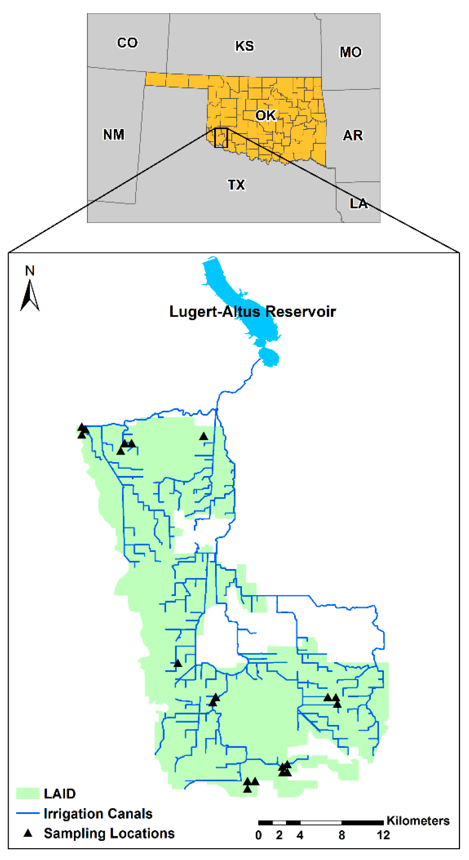
2.1. Study Area
2.2. Soil Sampling Procedure
2.3. Soil Testing Methods
2.4. Statistical Analysis
- I = 0 and S = 1: There is no change in the measured soil property by time (perfect stability),
- I ≠ 0 and S = 1: The mean soil property changed by time, and the change was spatially uniform (static),
- I = 0 and S ≠ 1: The mean soil property did not change by time, and changes at different locations were non-uniform (dynamic),
- I ≠ 0 and S ≠ 1: The mean soil property changed by time and the change was non-uniform (dynamic).
3. Results
3.1. Variations in Soil Chemical Properties
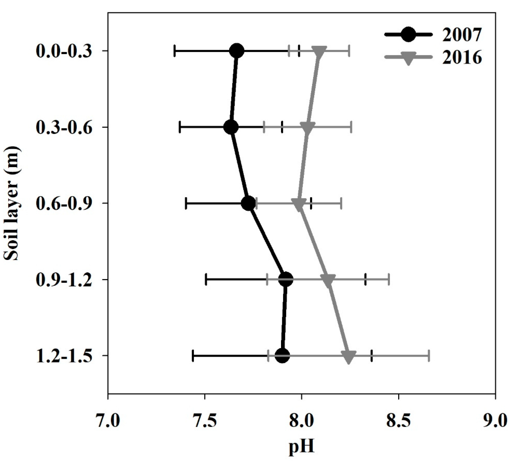
3.1.1. pH
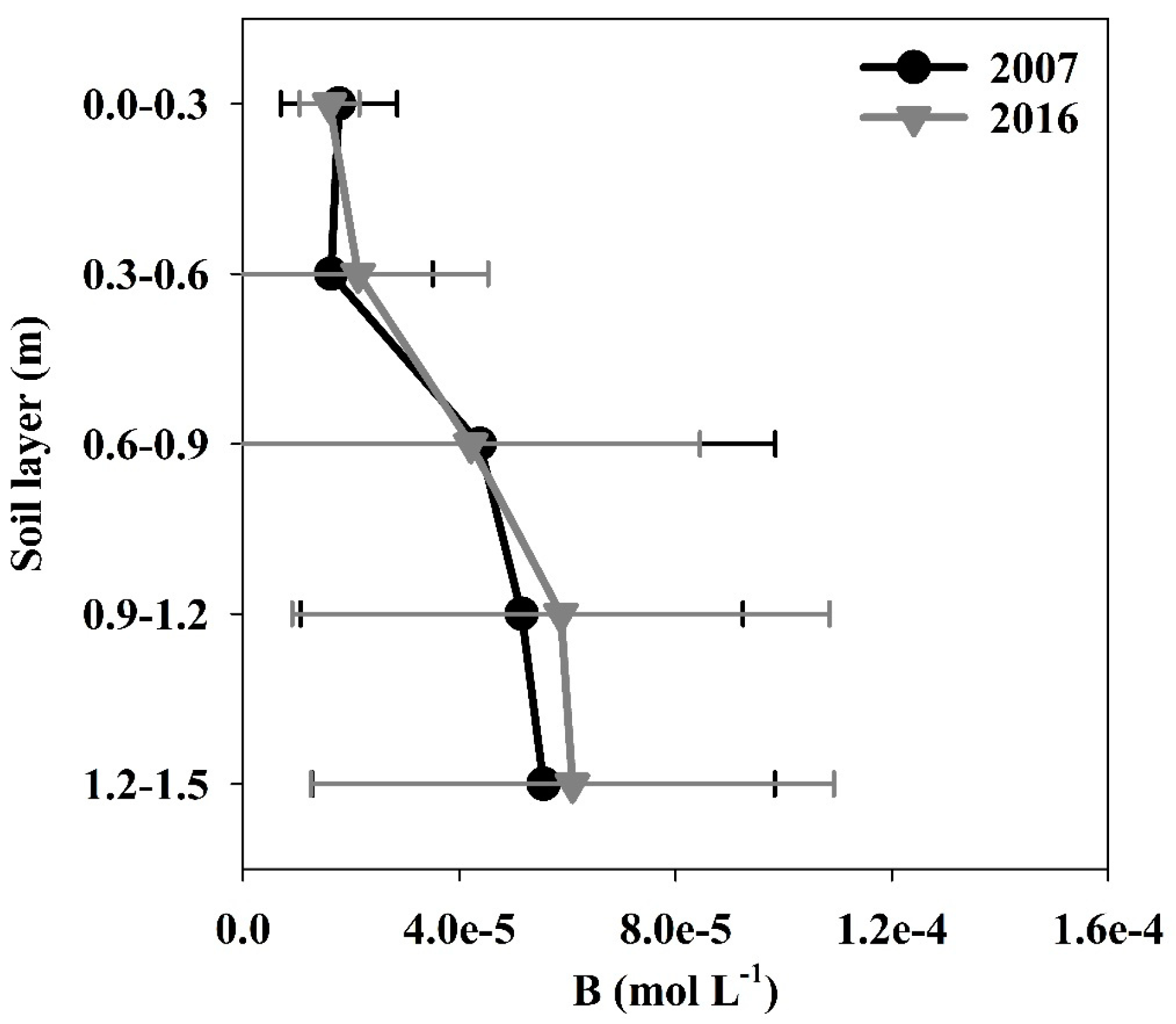
3.1.2. Boron
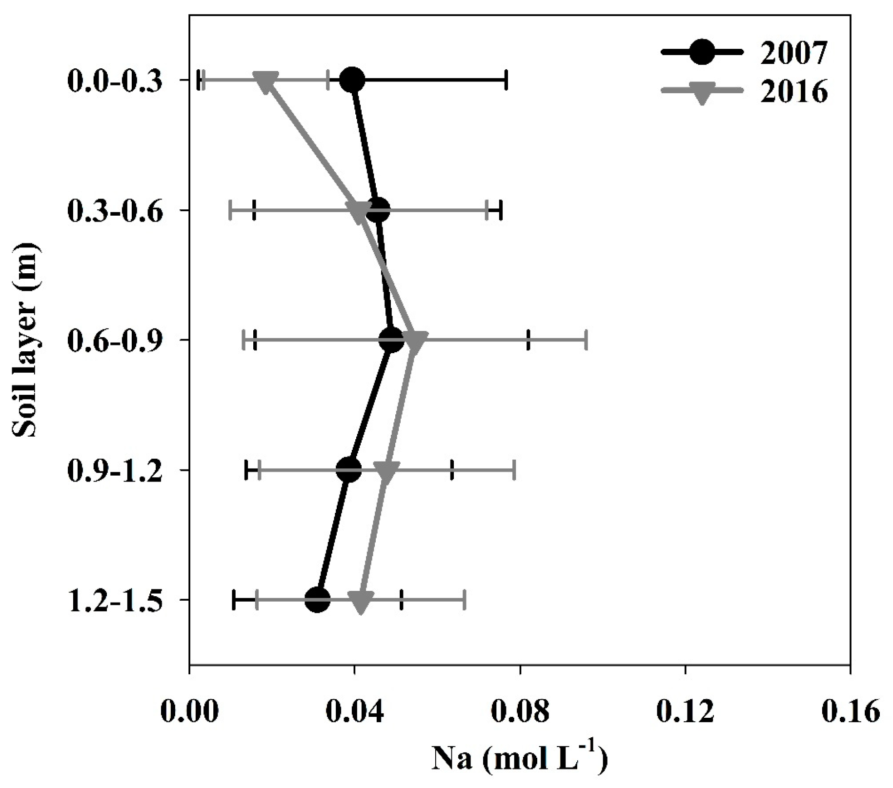
3.1.3. Sodium
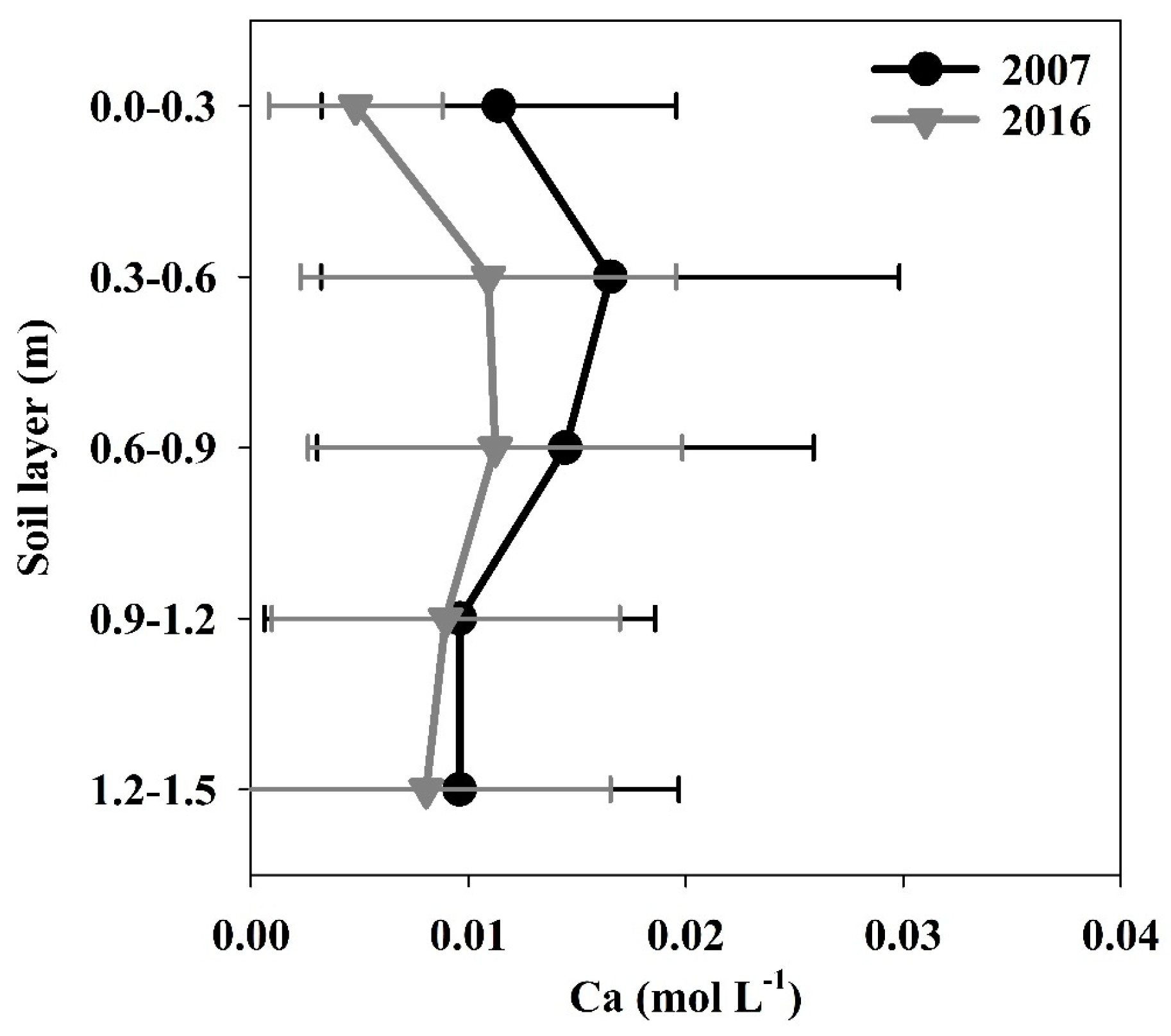
3.1.4. Calcium
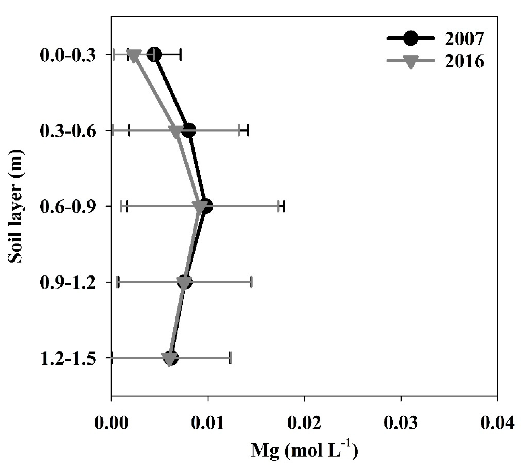
3.1.5. Magnesium
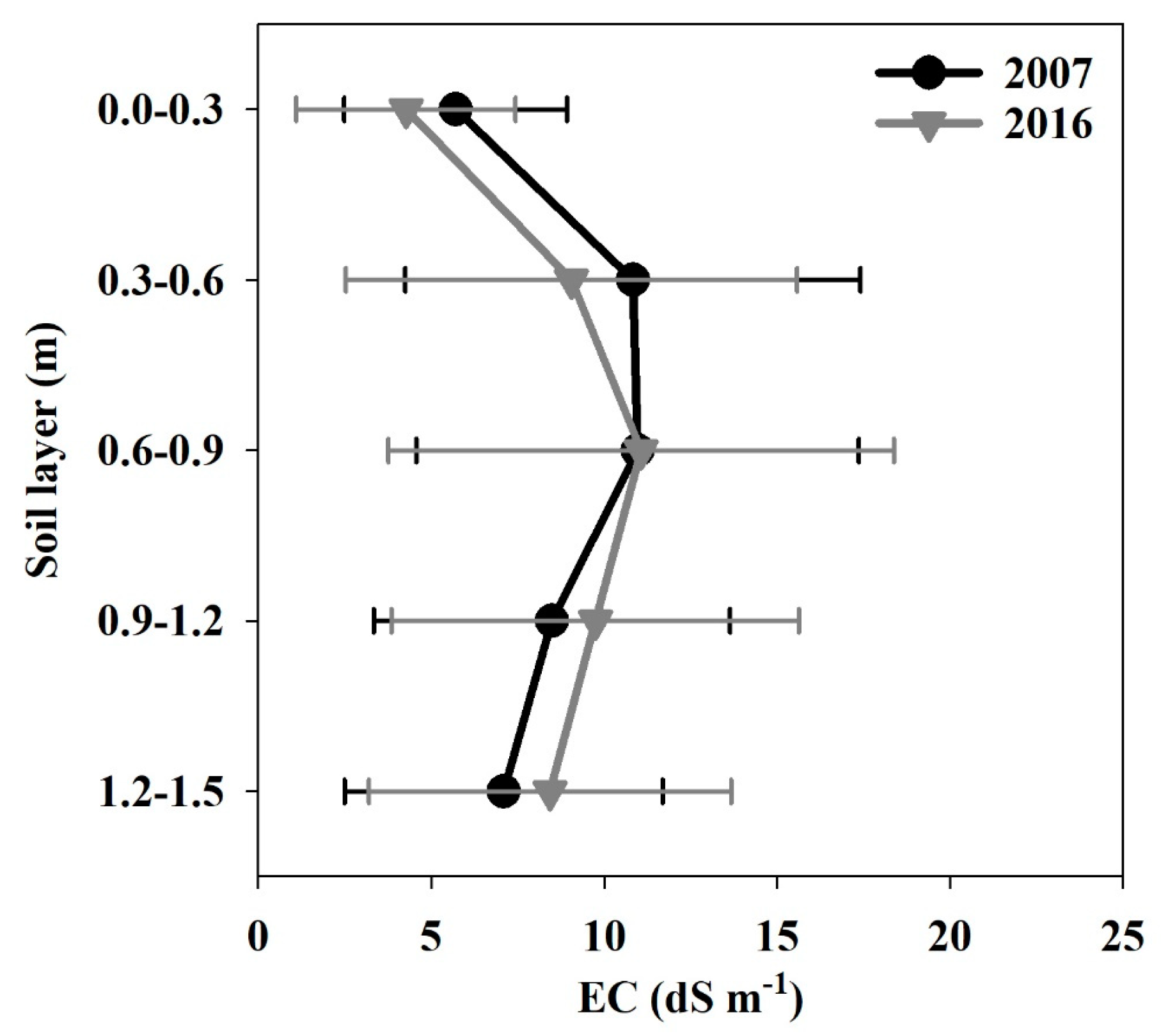
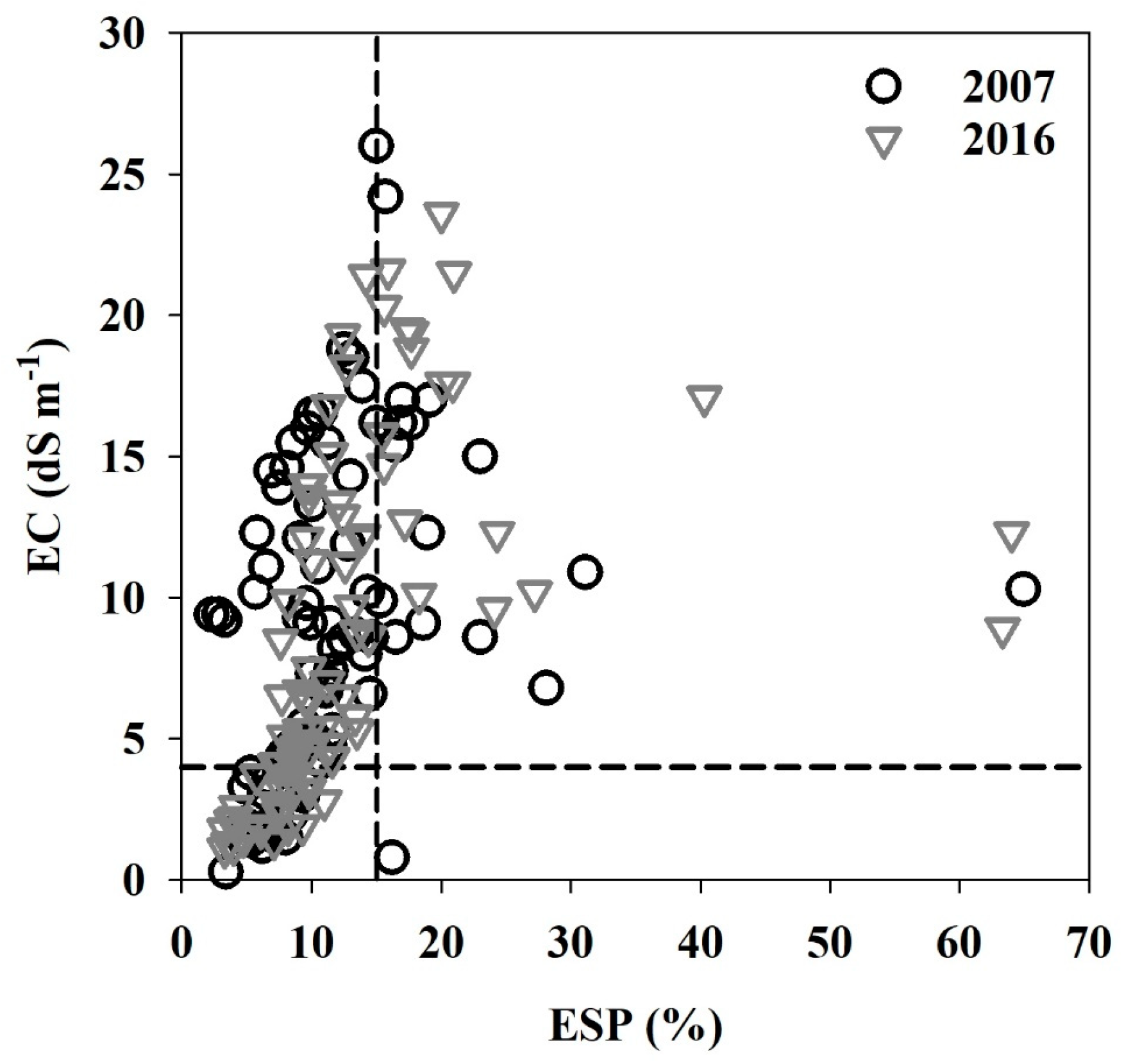
3.1.6. Electrical Conductivity
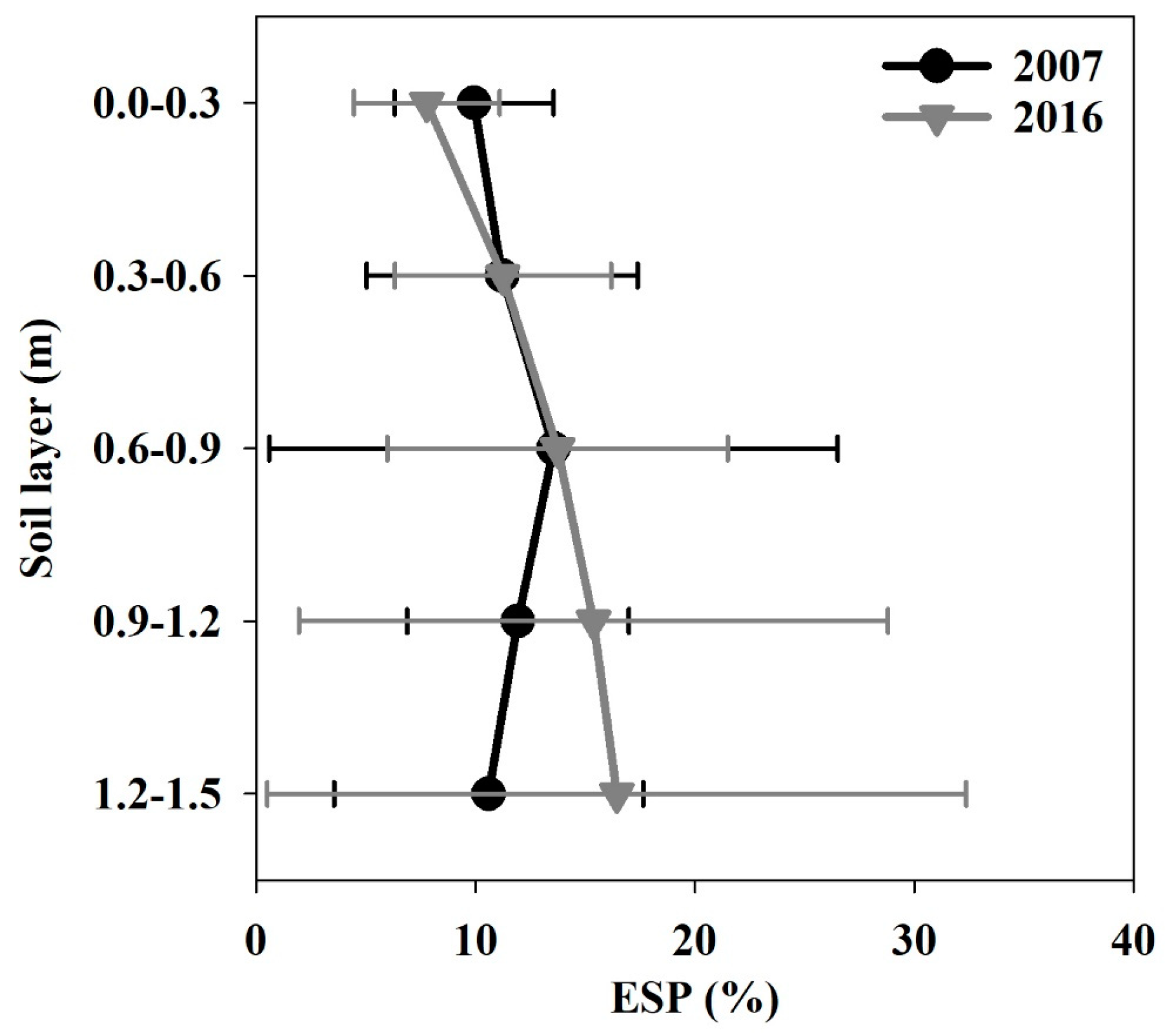
3.1.7. Exchangeable Sodium Percentage
3.2. Soil Salinity Classification
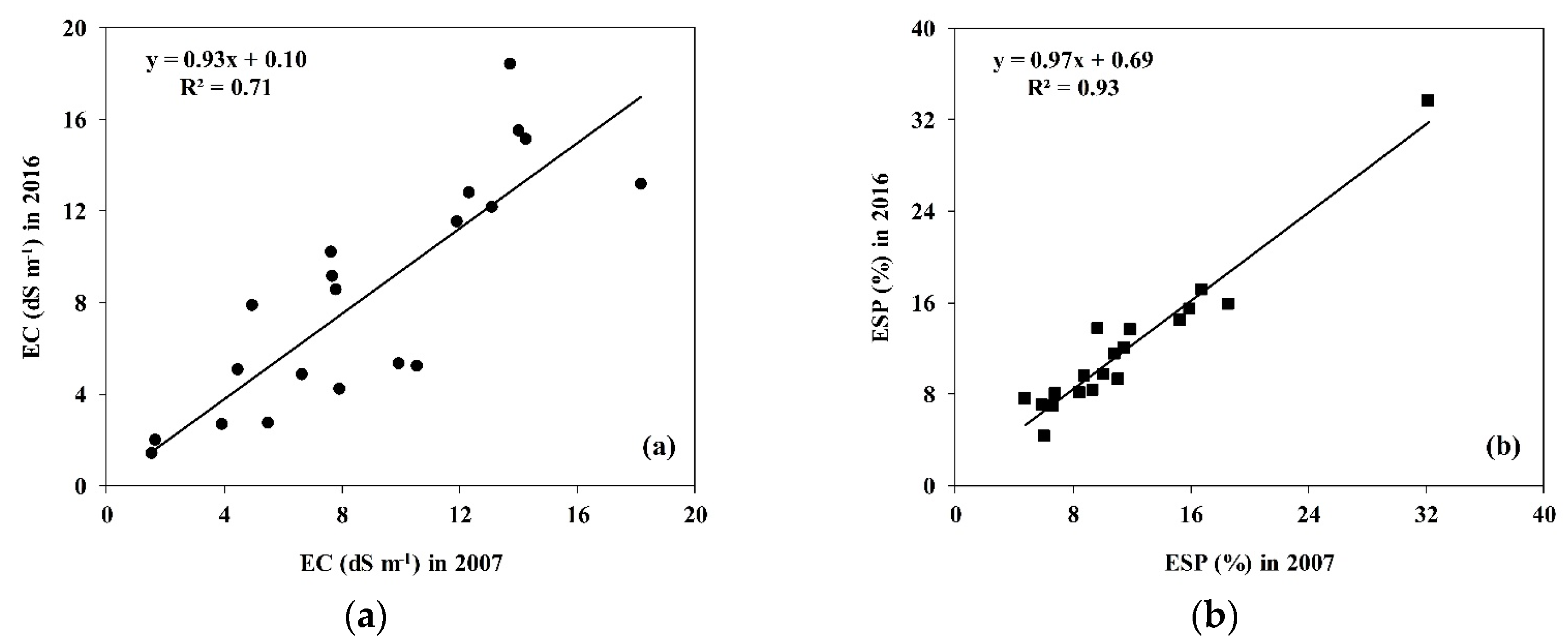
3.3. Temporal Stability
4. Conclusions
Author Contributions
Funding
Conflicts of Interest
References
- Ghassemi, F.; Jakeman, A.J.; Nix, H.A. Salinisation of Land and Water Resources: Human Causes, Extent, Management and Case Studies; CAB international: Wallingford, UK, 1995. [Google Scholar]
- Hillel, D. Salinity Management for Sustainable Irrigation: Integrating Science, Environment, and Economics; World Bank Publications: Washington, DC, USA, 2000. [Google Scholar]
- Tanji, K.K.; Kielen, N.C. Agricultural Drainage Water Management in Arid and Semi-Arid Areas; FAO: London, UK, 2002. [Google Scholar]
- Kijne, J.W. How to Manage Salinity in Irrigated Lands: A Selective Review with Particular Reference to Irrigation in Developing Countries; IWMI: Battaramulla, Sri Lanka, 1998. [Google Scholar]
- Oldeman, L.R.; Hakkeling, R.T.; Sombroek, W.G. World Map of the Status of Human-Induced Soil Degradation: An Explanatory Note; International Soil Reference and Information Centre: Wageningen, The Netherlands; United Nations Environment Programme: Nairobi, Kenya, 2017. [Google Scholar]
- Qadir, M.; Quillérou, E.; Nangia, V.; Murtaza, G.; Singh, M.; Thomas, R.J.; Drechsel, P.; Noble, A.D. Economics of salt-induced land degradation and restoration. Nat. Resour. Forum 2014, 38, 282–295. [Google Scholar] [CrossRef]
- Wallender, W.W.; Hopmans, J.W.; Grismer, M.E. Scales and scaling as a framework for synthesizing irrigated agroecosystem research on the westside San Joaquin Valley. In Salinity and Drainage in San Joaquin Valley, California; Springer: Dordrecht, The Netherlands, 2014; pp. 99–122. [Google Scholar]
- Feikema, P.M.; Baker, T.G. Effect of soil salinity on growth of irrigated plantation Eucalyptus in south-eastern Australia. Agric. Water Manag. 2011, 98, 1180–1188. [Google Scholar] [CrossRef]
- Razzouk, S.; Whittington, W.J. Effects of salinity on cotton yield and quality. Field Crops Res. 1991, 26, 305–314. [Google Scholar] [CrossRef]
- Tanton, W.T.; Rycroft, D.W.; Hashimi, M. Leaching of salt from a heavy clay subsoil under simulated rainfall conditions. Agric. Water Manag. 1995, 27, 321–329. [Google Scholar] [CrossRef]
- Armstrong, A.S.B.; Rycroft, D.W.; Tanton, T.W. Seasonal movement of salts in naturally structured saline-sodic clay soils. Agric. Water Manag. 1996, 32, 15–27. [Google Scholar] [CrossRef]
- Ballantyne, A.K. Movement of salts in agricultural soils of Saskatchewan 1964 to 1975. Can. J. Soil Sci. 1978, 58, 501–509. [Google Scholar] [CrossRef]
- Herrero, J.; Pérez-Coveta, O. Soil salinity changes over 24 years in a Mediterranean irrigated district. Geoderma 2005, 125, 287–308. [Google Scholar] [CrossRef]
- Wu, J.; Zhao, L.; Huang, J.; Yang, J.; Vincent, B.; Bouarfa, S.; Vidal, A. On the effectiveness of dry drainage in soil salinity control. Sci. China Ser. E Technol. Sci. 2009, 52, 3328–3334. [Google Scholar] [CrossRef]
- Autobee, R. The WC Austin Project; United States Bureau of Reclamation: Austin, TX, USA, 1994. [Google Scholar]
- USBR. Appraisal Report Water Supply Augmentation W.C. Austin Project, Oklahoma; United States Bureau of Reclamation: Austin, TX, USA, 2005.
- Masasi, B.; Taghvaeian, S.; Boman, R.; Datta, S. Impacts of Irrigation Termination Date on Cotton Yield and Irrigation Requirement. Agriculture 2019, 9, 39. [Google Scholar] [CrossRef]
- Evers, A.J.M.; Elliott, R.L.; Stevens, E.W. Integrated decision making for reservoir, irrigation, and crop management. Agric. Syst. 1998, 58, 529–554. [Google Scholar] [CrossRef]
- Taghvaeian, S.; Fox, G.; Boman, R.; Warren, J. Evaluating the impact of drought on surface and groundwater dependent irrigated agriculture in western Oklahoma. In 2015 ASABE/IA Irrigation Symposium: Emerging Technologies for Sustainable Irrigation-A Tribute to the Career of Terry Howell, Sr. Conference Proceedings; American Society of Agricultural and Biological Engineers: St. Joseph, MI, USA, 2015; pp. 1–8. [Google Scholar]
- Krueger, E.S.; Yimam, Y.T.; Ochsner, T.E. Human factors were dominant drivers of record low streamflow to a surface water irrigation district in the US southern Great Plains. Agric. Water Manag. 2017, 185, 93–104. [Google Scholar] [CrossRef]
- Richards, L.A. Diagnosis and Improvement of Saline and Alkali Soils; United States Department of Agriculture: Washington, DC, USA, 1954.
- Soltanpour, P.N.; Johnson, G.W.; Workman, S.M.; Jones, J.B.; Miller, R.O. Inductively coupled plasma emission spectrometry and inductively coupled plasma-mass spectrometry. In Methods of Soil Analysis. Part 3—Chemical Methods; Soil Science Society of America: Madison, WI, USA, 1996; pp. 91–139. [Google Scholar]
- Vachaud, G.; Passerat de Silans, A.; Balabanis, P.; Vauclin, M. Temporal stability of spatially measured soil water probability density function. Soil Sci. Soc. Am. 1985, 49, 822–828. [Google Scholar] [CrossRef]
- Ramsey, P.H. Critical values for Spearman’s Rank Order correlation. Educ. Stat. 1989, 14, 245–253. [Google Scholar]
- Kachanoski, R.G.; De Jong, E. Scale dependence and the temporal presistence of spatial patterns of soil water storgae. Water Resour. Res. 1989, 24, 85–91. [Google Scholar] [CrossRef]
- Douaik, A.; Van Meirvenne, M.; Tóth, T. Statistical Methods for Evaluating Soil Salinity Spatial and Temporal Variability. Soil Sci. Soc. Am. J. 2007, 71, 1629–1635. [Google Scholar] [CrossRef]
- Thomas, G.W. Soil pH and soil acidity. In Methods of Soil Analysis Part 3—Chemical Methods; Soil Science Society of America: Madison, WI, USA, 1996; pp. 475–490. [Google Scholar]
- Kent, L.M.; Lauchli, A. Germination and seedling growth of cotton: Salinity-calcium interactions. Plant Cell Environ. 1985, 8, 155–159. [Google Scholar] [CrossRef]
- Bohn, H.L.; Strawn, D.G.; O’Connor, G.A. Soil Chemistry; John Wiley and Sons: Hoboken, NJ, USA, 2001. [Google Scholar]
- Agricultural Salinity Assessment and Management; Wallender, W.W., Tanji, K.K., Eds.; American Society of Civil Engineers: Reston, VA, USA, 2011. [Google Scholar] [CrossRef]
- Ayers, R.S.; Westcot, D.W. Water Quality for Agriculture; Food and Agriculture Organization of the United Nations: Rome, Italy, 1985; p. 29. [Google Scholar]
- Maas, E.V. Salt Tolerance of Plants. In Handbook of Plant Science in Agriculture; Christie, B.R., Ed.; CRC Press: Boca Raton, FL, USA, 1987. [Google Scholar]
- Grattan, S.R. Irrigation with saline water. In Management of Water Use in Agriculture; Springer: Berlin, Germany, 1994. [Google Scholar]
- Ayars, J.E.; Hutmacher, R.B.; Schoneman, R.A.; Vail, S.S.; Pflaum, T. Long term use of saline water for irrigation. Irrig. Sci. 1993, 14, 27–34. [Google Scholar] [CrossRef]
- Moreno, F.; Cabrera, F.; Andrew, L.; Vaz, R.; Martin-Aranda, J.; Vachaud, G. Water movement and salt leaching in drained and irrigated marsh soils of southwest Spain. Agric. Water Manag. 1995, 27, 25–44. [Google Scholar] [CrossRef]
- Datta, S.; Taghvaeian, S.; Ochsner, T.E.; Moriasi, D.; Gowda, P.; Steiner, J.L. Performance Assessment of Five Different Soil Moisture Sensors under Irrigated Field Conditions in Oklahoma. Sensors 2018, 18, 3786. [Google Scholar] [CrossRef]
- Bernstein, L. Salt Tolerance of Field Crops; United States Department of Agriculture: Washington, DC, USA, 1960. [Google Scholar]
- Dodd, K.; Guppy, C.N.; Lockwood, P.V.; Rochester, I.J. The effect of sodicity on cotton: Does soil chemistry or soil physical condition have the greater role? Crop Pasture Sci. 2013, 64, 806–815. [Google Scholar] [CrossRef]
- Choudhary, O.P.; Josan, A.S.; Bajwa, M.S. Yield and fibre quality of cotton cultivars as affected by the build-up of sodium in the soils with sustained sodic irrigations under semi-arid conditions. Agric. Water Manag. 2001, 49, 1–9. [Google Scholar] [CrossRef]
- Abrol, I.P.; Yadav, J.S.P.; Massoud, F.I. Salt-Affected Soils and Their Management; Food & Agriculture Organization: Rome, Italy, 1988. [Google Scholar]
- Zhang, H. Reclaiming Slick-Spots and Salty Soils; Oklahoma Cooperative Extension Services Publication; Oklahoma State University: Stillwater, OK, USA, 2013; p. PSS-2226. [Google Scholar]
- Douaik, A.; Van Meirvenne, M.; Toth, T. Temporal stability of spatial patterns of soil salinity determined from laboratory and field electrolytic conductivity. Arid Land Res. Manag. 2006, 20, 1–13. [Google Scholar] [CrossRef]


| Parameter | Growing Season | Year |
|---|---|---|
| Total Prec. 1 (mm) | 322 | 610 |
| Mean Rs 2 (MJ m−2) | 21.8 | 17.0 |
| Min Tair 3 (°C) | 18.6 | 9.4 |
| Max Tair (°C) | 32.2 | 23.3 |
| Mean Tair (°C) | 25.2 | 16.1 |
| Min RH 4 (%) | 34.4 | 37.2 |
| Mean VPD 5 (kpa) | 1.6 | 1.0 |
| Mean U2 6 (m s−1) | 3.0 | 3.2 |
| Class | EC | ESP | Profile | 0.0–0.3 | 0.3–0.6 | 0.6–0.9 | 0.9–1.2 | 1.2–1.5 | ||||||
|---|---|---|---|---|---|---|---|---|---|---|---|---|---|---|
| 2007 | 2016 | 2007 | 2016 | 2007 | 2016 | 2007 | 2016 | 2007 | 2016 | 2007 | 2016 | |||
| Normal | <=4 | <=15 | 22 | 29 | 35 | 60 | 20 | 20 | 15 | 20 | 18 | 18 | 25 | 25 |
| Sodic | <=4 | >15 | 1 | 0 | 0 | 0 | 0 | 0 | 0 | 0 | 1 | 0 | 0 | 0 |
| Saline | >4 | <=15 | 60 | 50 | 55 | 35 | 60 | 60 | 60 | 45 | 65 | 59 | 58 | 50 |
| Saline-sodic | >4 | >15 | 17 | 21 | 10 | 5 | 20 | 20 | 25 | 35 | 12 | 24 | 17 | 25 |
| Parameter | rs |
|---|---|
| B | 0.761 |
| Ca | 0.687 |
| Mg | 0.877 |
| Na | 0.814 |
| pH | 0.781 |
| EC | 0.875 |
| ESP | 0.935 |
| Parameter | I | P (H0: I = 0) | S | P (H0: S = 1) | r2 |
|---|---|---|---|---|---|
| B | 0.02 | 0.589 | 1.00 | 0.499 | 0.86 |
| Ca | 113.6 | 0.235 | 0.46 | 0.001 1 | 0.34 |
| Mg | −14.1 | 0.580 | 0.93 | 0.292 | 0.78 |
| Na | 79.7 | 0.619 | 0.85 | 0.149 | 0.67 |
| pH | 4.11 | 0.000 1 | 0.51 | 0.000 1 | 0.72 |
| EC | 0.10 | 0.944 | 0.93 | 0.310 | 0.71 |
| ESP | 0.69 | 0.396 | 0.97 | 0.299 | 0.93 |
© 2019 by the authors. Licensee MDPI, Basel, Switzerland. This article is an open access article distributed under the terms and conditions of the Creative Commons Attribution (CC BY) license (http://creativecommons.org/licenses/by/4.0/).
Share and Cite
Chamaki, S.; Taghvaeian, S.; Zhang, H.; Warren, J.G. Soil Salinity Variations in an Irrigation Scheme during a Period of Extreme Dry and Wet Cycles. Soil Syst. 2019, 3, 35. https://doi.org/10.3390/soilsystems3020035
Chamaki S, Taghvaeian S, Zhang H, Warren JG. Soil Salinity Variations in an Irrigation Scheme during a Period of Extreme Dry and Wet Cycles. Soil Systems. 2019; 3(2):35. https://doi.org/10.3390/soilsystems3020035
Chicago/Turabian StyleChamaki, Sheyda, Saleh Taghvaeian, Hailin Zhang, and Jason G. Warren. 2019. "Soil Salinity Variations in an Irrigation Scheme during a Period of Extreme Dry and Wet Cycles" Soil Systems 3, no. 2: 35. https://doi.org/10.3390/soilsystems3020035
APA StyleChamaki, S., Taghvaeian, S., Zhang, H., & Warren, J. G. (2019). Soil Salinity Variations in an Irrigation Scheme during a Period of Extreme Dry and Wet Cycles. Soil Systems, 3(2), 35. https://doi.org/10.3390/soilsystems3020035