Article

What is the Best Inference Trajectory for Mapping Soil Functions: An Example of Mapping Soil Available Water Capacity over Languedoc Roussillon (France)

by
Quentin Styc
1,2,* and
Philippe Lagacherie
1
1
LISAH, University Montpellier, IRD, INRA, Montpellier SupAgro, 34060 Montpellier, France
2
BRL Exploitation, CEDEX 5, 30001 Nîmes, France
*
Author to whom correspondence should be addressed.
Soil Syst. 2019, 3(2), 34; https://doi.org/10.3390/soilsystems3020034
Submission received: 12 April 2019 / Revised: 30 April 2019 / Accepted: 1 May 2019 / Published: 7 May 2019
(This article belongs to the Special Issue Digital Soil Mapping of Soil Functions)

Abstract

:
Extending digital soil mapping to the mapping of soil functions that can support end-user decisions comes to coupling a digital soil mapping procedure and a soil function assessment method. This can be done following various possible inference trajectories following the order with which “combining primary soil properties”, “aggregating soil layers across depths” and “mapping” are executed to provide the targeted output. Eighteen inference trajectories, designed for computing soil available water capacity maps in the Languedoc–Roussillon region (France), were compared with regard to their mapping performances. The best performance (SSMSE = 0.42) was obtained by a trajectory that, before mapping, combined the three first GlobalSoilMap soil layers and computed the available water capacity of each layer. The worst (SSMSE = 0.07) was observed when all the soil layers and soil properties were combined prior to mapping. We explain the observed differences between trajectories by examining the differences in mapping errors and in error propagation between the compared trajectories, which involve both the correlations between the soil properties and between their mapping errors. This paves the way to spatial soil inference systems that could perform an ex ante selection of the best possible inference trajectory for mapping a soil function.

Graphical Abstract

1. Introduction

It is increasingly recognized that soils and their functions have a part to play in the large existential challenges that have been recognized for the sustainable development of humanity and planet Earth [1]. Addressing such challenges needs to appropriately informing local and global decision making, which requires a knowledge of soils at fine resolution and global extent [2]. Digital Soil Mapping (DSM) [3,4] has been proposed as a methodology for reaching this requirement. Various applications of DSM across the globe [5] demonstrated that DSM can now operationally produce sets of high resolution images representing the spatial variations of the most currently required soil properties or “primary soil properties” (e.g., soil textural fractions, soil carbon content, available water capacity, etc.).
In spite of these substantial efforts for moving to operationality, DSM has still not fully matched the initial objective. A new step is to shift from mapping primary soil properties to mapping soil functions. After the pioneering paper of Carré et al. [6] that advocated for digital soil assessment approaches, there has been abundant literature providing conceptual advances for the description of soil functions and the related ecosystem services [7] and also on the valuations of soil services [8]. Greiner et al. [9] recently proposed a set of soil function assessment (SFA) methods that cover the multiple functionalities of soils and are applicable to ecosystem service supply assessments. These SFA methods use as inputs a minimum set of primary soil properties and pedotransfer functions which makes them largely applicable provided that the spatial data on primary soil properties are made available. This carries implicitly the idea that (digital) soil mapping and soil function assessment methods are two independent processes that can be only loosely coupled through a straightforward transfer of data. This is this idea that we want to question in this paper.
Beyond their differences, all the SFA methods share a similar data flow. They provide a single output—the valuation of the soil function—from a set of soil properties that characterize different soil layers. 
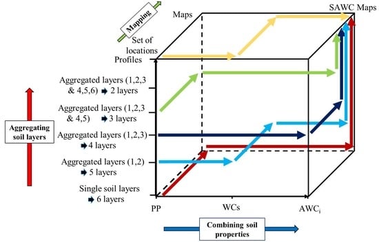
Figure 1 represents in a three-dimensional space the different possible inference trajectories that can be envisaged for producing an SFA output, with the inclusion of the mapping process in these trajectories. The inference trajectories may differ in the order with which “combining primary soil properties”, “aggregating soil layers across depths”, and “mapping” are executed to provide the common targeted SFA output. The commonly followed approach, i.e., mapping first then combining soil property and aggregating soil layers, is one of the possible trajectories (shown in green on Figure 1), but many others exist. Mapping could be the last executed process after having combined the soil properties and the soil layers over the soil input dataset (“mapping last” in blue on Figure 1). Combining first the soil properties at each single soil layer, then mapping and lastly aggregating SFA outputs is an intermediate inference trajectory (shown in red on Figure 1) that can be envisaged too. Apart from these three examples, one can imagine a large number of other inference trajectories since both partial combinations of soil properties and partial aggregations of soil layers can be envisaged.
Considering that SFA could be applied following these different mapping trajectories, the following question comes; “which inference trajectory provides the most accurate SFA output?” Recently, Laborczi et al. [10] provided a partial response to this question. They compared two inference trajectories for mapping sand, silt and clay content at 0–30 cm depth, which consisted of either first aggregating the GlobalSoilMap layers (0–5 cm, 5–15 cm, and 15–30 cm) then mapping or first mapping each individual layer and then aggregating the layers. They obtained significantly different outputs between the different trajectories, the former trajectory providing slightly worse predictions than the latter one. To our knowledge, such a comparison has not been extended yet to a more generic case study involving the whole inference trajectories for computing soil functions.
In this paper, we address the above evoked question by taking as an example the mapping of the soil available water capacity (SAWC) of a soil profile. Although SAWC cannot be considered as a soil function per se, it shares the same issues of the choice of inference trajectories. Furthermore, SAWC is involved in the assessment of several ecosystem services [7], either provisioning services—food, fuel, and fiber production—or regulating services—climate and gas regulation, water regulation, or erosion and flood control. SAWC is mapped over the Languedoc–Roussillon region using the same inputs as earlier DSM papers dealing with the same region [11,12].

2. The Problem

SAWC is a well-known concept that has been used for a long time to express the capacity of soils to store water for plants [13]; SAWC is computed using a classic expression:
S A W C =   i = 1 n d h i b d i ( 100 s t i 100 ) ( θ r i θ w i )
where SAWC is the soil available water capacity (cm), d h i   = thickness of the ith horizon (cm), b d i = bulk density of the ith horizon, s t i = coarse fragment content of the ith horizon (% volumetric), and θ r i and θ w i are soil water contents at field capacity (FC) and at permanent wilting point (PWP) of the ith horizon (cm3.cm−3), respectively.
When the mapping of SAWC is targeted, some modifications to Equation (1) are necessary.
First, bulk density, soil water contents at FC and at PWP are expensive to measure soil properties that are rarely available in current soil databases, which prevent their mapping. The alternative solution is to estimate these data from more easily mappable primary soil properties (e.g., particle size fractions and organic carbon) by using pedotransfer functions (PTFs) [14]. Many PTFs have been developed for estimating the soil properties required for computing SAWC [15,16]. In particular, PTFs can be used to calculate volumetric water contents at FC and PWP (e.g., Wösten et al. [15]), which embeds the bulk density information and avoids using a specific PTF to estimate bulk density. Volumetric water contents are estimated as follows
θ r i =   j = 1 n α j P P j +   ε
θ w i =   j = 1 n α j P P j +   ε
where θ r i = volumetric soil water content at FC (cm3.cm−3), θ w i = volumetric soil water content at PWP (cm3.cm−3), α 1   α n = the coefficient of the model, P P 1 P P n is the value of the selected primary soil properties as input, and ε is an estimated error.
A second modification of Equation (1) is the replacement of horizons whose thicknesses are variable across locations by soil layers with fixed depths. This has been introduced in digital soil mapping as a simple way for dealing with soil variability across depths [17]. The general principle is to fit a continuous depth function (spline) of a given property onto the values of the property for the successive horizons, which allows further estimations of the soil properties for any possible layer defined by a user-fixed interval of depth [18]. This enables the harmonization of soil depths intervals across DSM input locations, which greatly facilitates further mapping. A discretization into six layers (0–5, 5–15, 15–30, 30–60, and 60–100 cm) has been adopted in the specifications of the GlobalSoilMap project [19], which has made this discretization the most commonly applied.
When PTFs and fixed depth soil layers are introduced in the SAWC formula, we obtain the following formula.
S A W C =   i = 1 n S L h i ( 100 s t i 100 )   [ ( j = 1 n α j P P j +   ε ) ( j = 1 n α j P P j +   ε ) ]
where S L h i is the thickness of soil layers fixed by soil depth interval for i = 1 , , 6 when the specifications of the GlobalSoilMap project are followed.
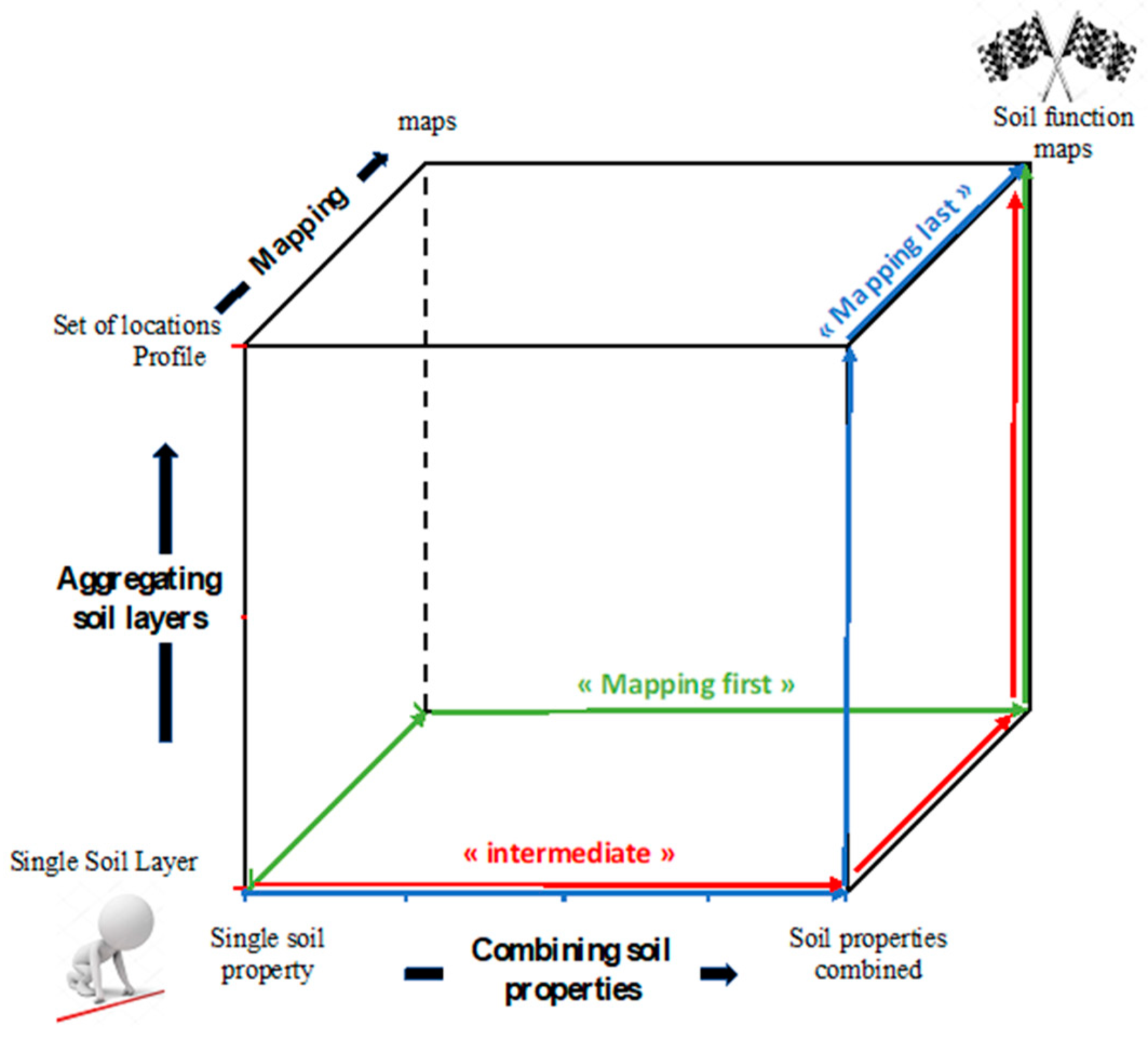
From Equation (4), the variety of possible inference trajectories for mapping SAWC can be represented as an implementation of Figure 1 (Figure 2). The blue axis shows three different ways to combine soil properties (the most straightforward ones, among others): (1) considering primary property (PP), i.e., no combination; (2) considering the volumetric soil water contents at FC and PWP (WCs), i.e., application of PTFs first; and (3) considering the available water capacity of a given soil layer i (AWCi), i.e., whole application of Equation (4) first. On the red axis, we have six possibilities for soil discretization across depths (the most straightforward, among others): from considering the six GlobalSoilMap-fixed soil layers, i.e., no combination, to a full aggregation of soil layers, i.e., aggregating layers to soil profile first. Four other possibilities are considered by merging an increasing number of layers (Figure 2).
From Figure 2, it is possible to define 18 possible inference trajectories for mapping SAWC, i.e., three modalities of property combinations x six modalities of combining soil layers. For the sake of readability, only five out of these 18 trajectories are presented in Figure 2. It must be noted that the most classic inference trajectory (mapping first then aggregating properties and layers), which fully dissociate mapping and SAWC computing, was included among the 18 tested strategies.
In this paper, we investigated whether these different inference trajectories provided similar results or not, the input data and the underlying formula (Equation (4)) being the same for all trajectories. If not, we also wanted to know which trajectory provided the best mapping performance.

2.1. The Case Study

2.1.1. Study Area

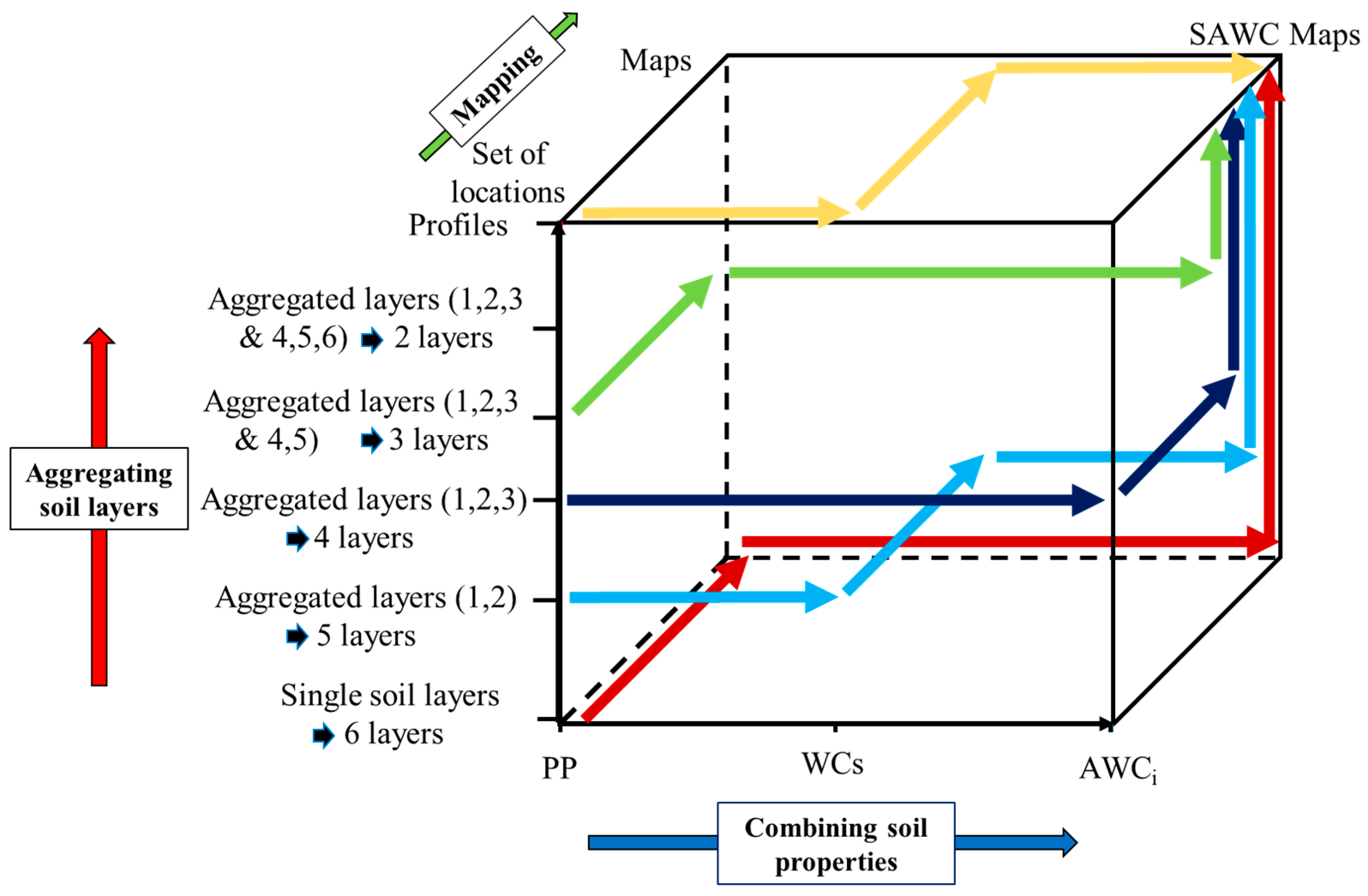
Languedoc–Roussillon is one of the 22 former administrative regions in France (Figure 3), and is now part of the country’s newest region, Occitanie, which resulted from the merging of Languedoc Roussillon and Midi-Pyrénées. Located in Southern France, it covers 27,236 km² of land and stretches from the Mediterranean Sea to the Pyrenees and to the Massif Central Mountains. The region includes a wide variety of climates, parent materials and landscapes: low sedimentary plains with vineyards and/or cereals, dry limestone plateaus with scrublands and evergreen oak forests, slopes of Paleozoic mountains covered by forests, and volcanic and granitic highlands with grasslands. The soil cover of the region is consequently very diverse, including 18 WRB major soil groups that represent 56% and 75% of the total number of the soil group populations in the world and in Europe, respectively.

2.1.2. Soil Data Input

In this study, we used a legacy dataset of 640 measured soil profiles selected from the 2024 used in Vaysse and Lagacherie [11,12]. This selection was made to ensure that the same input data was used by all of the inference trajectories. This motivated to select only the profiles that were fully documented for each soil property and for each layer. Indeed, this restrictive condition was necessary for providing non-null inputs for applying the “combine first” inference trajectory (i.e., combining all soil properties and for all soil layers before mapping). Finally, the density of this dataset of the study area was one soil profile for each 41 km².

Documenting Soil Layer Thickness

The soil layer thicknesses (Equation (4)) that were initially defined through the fixed interval depth, 5, 10, 15, 30, 40, and 100 cm for layers 1 to 6, respectively, needed to be updated to account for soils having a depth less than 200 cm. This was done from the following formula.
If   S D > U L i ,   then   S L h i = U L i L L i If   U L i > S D > L L i ,   then   S L h i = S D L L i .   If   S D < L L i ,   then   S L h i = 0 .
where SD is the soil depth, S L h i is the soil thickness of the soil layer and, U L i and L L i are the upper and lower limits of the considered soil layer, respectively.
Equation (5) requires first to document the soil depth (SD), i.e., the distance (in cm) from the soil surface to the bedrock or a paralithic contact [20]. This was done by a prior classification tree that determined whether or not the bottom horizon could be considered as bedrock or as a paralithic contact. Figure 4 shows the decision tree that was used for classifying the bottom horizon. The type of soil horizon was first used to identify lithic (R, M or D) vs. pedological horizons. Since the horizon type, C, remained ambiguous with respect to the targeted classification, additional soil variables were used (types of structure, compaction, and weathering), which allowed for the identification of paralithic horizons vs. pedological horizons.
From this classification of horizons, the soil depths were determined by applying the following rules:
  • If the bottom horizon is lithic or paralithic, then the soil depth is the upper depth of the bottom horizon.
  • If the bottom horizon is still a pedological one, the soil depth cannot be determined and thus the site is not selected. A total of 760 measured soil profiles were removed for this reason, which corresponded to 55% of the total removal of sites.

Documenting Layers with the Other Required Soil Properties

As the described pedological horizons available in the soil database were defined by variable soil depths, a prior interpolation was required to document the soil layers. Spline functions work as an interpolator, respecting the average values of the target soil property, and assuming a continuous variation with depth [13]. As an outcome, spline functions deliver a set of interpolated values at specific depths which are, in our study, the depth intervals provided by GlobalSoilMap.net specifications (0–5, 5–15, 15–30, 30–60, 60–100, and 100–200 cm). Then, the mass-preserving spline functions were applied to clay, silt, sand, and coarse fragment contents.
The values of the soil properties for the tested aggregated layers (see Figure 2) were derived from their values at the six depth intervals using a weighted mean by soil layer thickness.

Local Continuous PTFs

As presented in Section 2, the common way to obtain soil water contents, that partially drives AWC (i.e., soil water contents at FC and PWP), is to use pedotransfer functions. The continuous PTFs used in this study are obtained from an investigation based on the analysis of a dataset of 294 pedological horizons belonging to 115 soil profiles located in the Hérault River Valley in the former Languedoc Roussillon region [21]. The dataset contained soil water volumetric contents at FC (10 kPa) and at PWP (1500 kPa), particle size fractions (clay, silt, and sand), bulk density, and organic carbon content. Before starting the investigation, bulk density and organic carbon were discarded from the dataset because not all horizons of the STIPA database reported their values, making PTFs inapplicable for local prediction. PTFs were fitted using a point estimation approach based on multiple linear regression carried out with the stats R package [22]. Model variables were selected using the Akaike’s information criterion (AIC) [23] applied to a backward/forward stepwise procedure. Linearity was visually analyzed on linear model graphs, then tested with the RESET test for nonlinearity [24]. Linear models that fitted to the data set are reported in Table 1. Since particle size fractions are compositional data, stepwise selection will always remove at least one of them from the model. In this case, clay was selected for both models, sand better explained water content at field capacity predictions, and silt, water content at permanent wilting point predictions. Performance assessments showed great performances for both PTFs, with a certain advantage for PWP’s PTF.

2.1.3. Soil Covariates

The DSM process used in this study is based on the well-known scorpan model [3] that uses quantitative relationships between targeted soil property and environmental variables also called “covariates”.
The selection of the landscape covariates (Table 2) had been performed for a previous DSM application in the region [11]. It was based on two criteria: (i) the covariates could be derived from freely available geodatasets, at least at the French national level, and (ii) they have a logical and deterministic relationship to the soil properties, according to the literature.
Classical geomorphometric indicators found in the DSM literature were computed from the global Shuttle Radar Topographic Mission (SRTM) digital elevation model (DEM): the elevation, slope, plan curvature, profile curvature, set of multiresolution valley bottom flatness (MRVBF), set of multiresolution ridge top flatness (MRRTF), topographic position index, and topographic wetness index.
The parent materials were characterized from the National Geological 1:50,000 map obtained from the French Geological Survey [25]. This map was translated into three parent material soil covariates, namely, the hardness, mineralogy and texture of alteration materials, following a mixed approach that involved both our pedologic knowledge and the measured legacy profiles described above (see details in Vaysse and Lagacherie [11]).
Land use was mapped across the region by a manual interpretation of Landsat 7 images from 2006. The initial classification into 43 land use types was condensed into nine types that were considered to be correlated with soil variations (e.g., artificial areas, greenhouse cultivation, permanent crops and orchards, forests, heathlands and pastures, scrublands, wetlands, complex territories composed of natural and agricultural areas, and forests in transition).
The basic climate data (maximum temperature, minimum temperature, and precipitation) were extracted from the Global Climate Database at a resolution of 1 km2 [26]. Two aridity indexes were derived from these data, namely, the De Martonne index and the Emberger index (see details in Vaysse and Lagacherie [11]).
Additionally, we added to the covariate set the regional-scale soil map (1:250,000) that regroups the major landscape types across the region.

3. Methods

3.1. Mapping Model: Quantile Regression Forest

The mapping model selected for this work is the Quantile Random Forest (QRF) [27], which is a very popular machine-learning algorithm in recent DSM operational applications [11,12,28].
In this section, we first describe the random forest algorithm [29] from which QRF was extended and then provide the specific features of QRF. In the following, we use excerpts from Meinshausen [27] to present these algorithms. More details can be found in this paper.
We let Y be a real-valued response variable and X be a covariate or predictor variable. A standard goal of statistical analysis is to infer the relationship between Y and X. The random forest algorithm grows a large ensemble of decision trees using n independent observations (Yi, Xi), i = 1, …, n.
For each tree and each node, the random forest algorithm implements a random selection to determine a variable at which to split. For each tree, a bagged version of the training data is used. In addition, only a random subset of predictor variables is considered for the split point selection at each node. For regression, the prediction of a single tree of the random forest algorithm for a new data point, X = x, can be represented as the weighted average of the original observations Yi, i = 1, …, n:
μ ^ ( x ) =   i = 1 n w i ( x ,   θ ) Y i
where wi(x,θ) is the weight vector given by a positive constant if the observation Xi is part of the same leaf of the tree built from the random vector of variables in which X was dropped and is otherwise 0. Using the RF algorithm, the conditional mean, E(Y |X = x), is approximated by the averaged predictions of k individual trees, each constructed with an independent and identically distributed vector t, t = 1,…, k. We let wi(x) be the average of wi(T) over such a collection of trees:
w i ( x ) =   k 1 t = 1 n w i ( x , θ t )
The final predictions are the average of predictions of individual trees [29,30,31]:
μ ^ ( x ) =   i = 1 n w i ( x ) Y i
Recently, Wright, and Ziegler (2015) developed a fast implementation of Breiman’s random forest [29] and Meinshausen’s quantile regression forest [27], for high-dimensional data, which is available as the ranger R package [32]. This implementation is faster than QRF in terms of i) superior scaling of the number of samples, trees, and descriptive variables tried for splitting and ii) runtime and memory usage (see details in Wright and Ziegler [32]).
QRF was applied for mapping all possible soil properties considered in the inference trajectories. In particular, the thicknesses of soil layers ( S L h i in Equation (4)) were mapped separately so that all trajectories could be applied. However, the thicknesses of the upper soil layers (0–5 cm, 5–15 cm, 15–30 cm, 0–15 cm, and 0–30 cm) were not variable enough across the region for mapping (variance < 20 cm2). In that case, the predicted values at each location were fixed as the mean soil layer thickness.

3.2. Evaluation Protocol

The performances of digital mapping of SAWC and of all its components (primary soil properties, hydraulic properties (soil water contents at FC and PWP for different soil layers)) were evaluated by a k-fold cross validation. This evaluation procedure involves randomly dividing the data into k subsets. Then, the holdout method is repeated k times, such that each time one of the k subsets is used as the evaluation set, the other k-1 subsets are merged to form the calibration set. Following this procedure, every data point is included in an evaluation set exactly once and is included in a calibration set k-1 times. In our case, we choose k = 10 and, to increase the robustness of the evaluation, the 10-fold cross-validation was repeated 20 times. The k-fold cross validation was performed using the cvTools R package [33].
To evaluate the prediction performances, we used classic performance indicators, e.g., mean square error skill score (SSMSE) [28] that has the same interpretation than the percentage of variance explained by the model, root mean square error (RMSE) and bias.
The performance indicators were calculated for each of the 20 iterations and then averaged to obtain a final pooled value.
Since soil compartment differs from one AWC mapping trajectory to another, soil properties and AWC were predicted for varying soil layers. The evaluation protocol was adapted accordingly.

4. Results

4.1. Preliminary Results

In this section, we present basic statistics of the soil properties used for calculating as well as their correlations. We focused on correlations since they play a major role in error propagation [34], which, therefore, can be of great interest for comparing the performance of the tested inference trajectories.

4.1.1. Basic Statistics

We provide in Table 3 the basic statistics of the study area. Languedoc Roussillon presents soil texture with predominant sand fraction and significant amount of coarse fragment content, which varies consequently.

4.1.2. Correlation Tables of Input Data: Combining Soil Properties

Table 4 shows the averaged correlations between the properties involved in the SAWC computing (Equation (4)) with standard deviations that show the variations in correlation across the different considered soil layers. Soil thickness was independent of the other properties, whereas the coarse fragment content was weakly, but significantly, correlated with silt and sand. Additionally, sand content was highly negatively correlated to silt and clay contents. As expected, FC and PWP showed high correlations with the input properties of their PTFs (Table 1) and with each other, as the result of application of PTFs that used the same properties or strongly correlated ones (Table 1). Low standard deviations of all these correlations revealed their low variations across the soil layers.

4.1.3. Correlation Tables of Input Data: Aggregating Soil Layers

Table 5 shows the averaged correlations of properties between soil layers with standard deviations that show the variations in correlation across the soil properties. The three upper layers were greatly correlated while the correlations decreased for the deeper layers.

4.2. Primary and Hydric Property Mapping Performances

For the trajectories that did not map the SAWC but rather its components, Table 6 provides a summary of the performances obtained for each property across the different numbers of soil layers. For sake of readability, only SSMSE values are shown with mean, min, and max values across the set of trajectories with different numbers of soil layers. Concerning the primary soil properties, particle size fractions mapping exhibited the best performances, while coarse fragment content and soil thickness were very badly mapped. The hydraulic properties showed slightly similar results to those of particle size fractions from which they are derived.
It is also interesting to examine the correlations between mapping errors across properties and layers since, according to the error propagation formula [34], it plays a role in the final errors on AWC. Table 7 shows the correlations between mapping residuals for the soil properties used in the trajectories. High correlations of residuals were observed between sand and the two other textural fractions, whereas moderate but significant correlations of residuals can be noticed between coarse fragment and two of the textural fractions (silt and sand).
Table 8 presents averaged correlations of property residuals between the six GlobalSoilMap soil layers across the set of soil properties with their associated standard deviation. The pattern of correlation of the soil properties residuals between layers is similar to the one drawn by the correlation of input data (Table 4), i.e., (i) the great correlation of surface soil layers and (ii) decreasing correlation when the residuals correlation coefficient between aggregated layers drops below 0.9.

4.3. SAWC Mapping Trajectories Performance Comparisons

In this study, we tested 18 SAWC mapping trajectories. Table 9 shows the indicators of performance, SSMSE, RMSE, and Bias of the 18 tested trajectories with their mean values and standard deviations across the 20 iterations of the evaluation protocol.
The results showed substantial differences in performance across the tested trajectories (SSMSE between 0.08 and 0.42). These differences occurred both between trajectories that mapped different soil properties (SL.PP, SL.WC, and SL.AWC) and between trajectories that did not consider the same number of layers, although the former often exhibited differences that could be interpreted as being within the error margin of the evaluation process [35]. Roughly the same hierarchy of performances was found whatever the examined indicator.
Concerning the differences in performance between trajectories that mapped different soil properties, the best performances were mainly obtained by calculating first an AWC (SL.AWC) then mapping, although mapping the soil properties first (SL.PP) seems slightly better than calculating AWC first for the six-layer trajectory. However, this ranking should be considered with care because of the above noticed small differences of performances. Concerning the difference in performance between trajectories that do not consider the same number of layers, the maximum performances were obtained by considering four soil layers. The performances increased moderately from the six-layer trajectory to the four-layer trajectory, i.e., from SSMSE = 0.33 to SSMSE = 0.42 for SL.AWC trajectories and then dramatically decreased from the three-layer trajectory to the one-layer-trajectory, i.e., from SSMSE = 0.39 to SSMSE = 0.07 for SL.AWC trajectories.
According to the performance indicators, the best performance was obtained by an intermediate trajectory that considered four soil layers and mapped SAWC. It is also interesting to note that the classic trajectory, i.e., using DSM outputs for calculating a spatialized SAWC (the SL.PP trajectory with six layers) was not the best among the 18 tested.

5. Discussion

5.1. Level of Performances and Limitations

5.1.1. Level of Performances in Predicting Primary Soil Properties

In this study, we considered inference trajectories that involved mapping of soil primary properties by using a DSM model. The partial results presented in Section 4.2 can then be compared to those of previous studies in similar conditions. The performances delivered for particle size fractions were slightly worse than those provided recently by Román Dobarco et al. [36] for all of France (R² = 0.27, 0.43, and 0.46 for clay, silt, and sand content, respectively) with, however, the same hierarchy between sand, silt, and clay mapping performances. Vaysse and Lagacherie [11] obtained in the same study area better mapping performances for particle size fractions (between 0.19 and 0.36) but the same poor performances for thickness and coarse fragment, however, with another validation technique (independent validation test instead of cross validation). A comparison with results from Vaysse and Lagacherie [12] that used a cross validation confirmed the previous results for a given soil property (clay content for the 5–15 cm layer). The performance gap could be explained by the reduction in the size of the input dataset between Vaysse and Lagacherie [12] applications and this study (from 1945 to 640).

5.1.2. Level of Performance in Predicting SAWC

Among the 18 inference trajectories, the most appropriate for predicting SAWC was the one considering four soil layers (e.g., 0–30, 30–60, 60–100, and 100–200 cm) to directly predict SAWC. This trajectory obtained much better results than any mapping of SAWC components, i.e., individual soil properties at a given depth. This can be explained by the removal of intraprofile variabilities and noise that did not play any more when SAWC is considered.
In addition, this inference trajectory exhibited similar results to those obtained by Leenhardt et al. [21] with a R² ranges from 0.36 to 0.45 according to the scale of the SAWC map chosen. Except for this study, evaluation of SAWC mapping has rarely been applied and this paper is, to our knowledge, among the first that has performed such an evaluation. However, this evaluation remains incomplete since we did not take into account the error of the PTFs coefficient applied. However, Román Dobarco [36] found that PTF error played a minor role in SAWC mapping error.

5.2. Drivers of the Variability in Performance between Trajectories

The results exhibited substantial differences of mapping performance across the tested inference trajectories (Table 9). The most important differences in performance were observed when different numbers of soil layers were considered. The best performances were obtained when highly correlated soil layers (correlation >0.9 between layers 1, 2, and 3, cf. Table 5) were merged before mapping whereas the worst ones were obtained when fewer correlated soil layers were merged (correlation < 0.80 between layers, Table 5). The former came from averaging the DSM model inputs, which may decrease the input errors of the DSM models whereas the latter forced the DSM models to cope with contradictory drivers of the combined soil layer, which could negatively impact the performance. This result is partially in accordance with Heuvelink & Pebesma [37] who advocated a mapping first trajectory since it “enables a more efficient use of the spatial characteristics of the individual inputs”. We however brought a nuance to this statement by considering a correlation threshold beyond which combining first could be a better solution. These differences were not modified by the further combination of the soil layer maps for calculating the final SAWC since no noticeable differences were observed in mapping error correlations (Table 8) that could have created differences in error propagation through this additive operation [34].
The differences in performance observed between trajectories that mapped different soil properties (primary soil properties, hydraulic properties, or SAWC) were more difficult to interpret. First the differences in mapping performance were much smaller than previously observed. Furthermore, in contrast to the combination of soil layers, the combination of soil properties is multiplicative (Equation (4)). Therefore, the impacts of the correlations between soil properties and between their mapping errors could be very different.
More comparisons of such inference trajectories involving contrasted mapping results and a larger range of soil function expressions would be necessary for a full understanding and an ex ante prediction of the hierarchy of performances across the trajectories.
Finally, it must be noticed that the comparisons of the inference trajectories “all things being equal” required considering the same number of measured soil profiles across trajectories. This corresponded to the number of fully complete measured soil profiles that were necessary for mapping SAWC after combining all soil properties and all soil layers. However, other less restrictive inference strategies could use more locations for mapping some of the SAWC components. Indeed, mapping separately the soil properties at each soil layer would allow an increase in the amount of input data which could increase the mapping performance of some SAWC components and, in turn, might have a positive effect on the overall performances. However, this reasoning does not hold for the depth prediction that is still limited by the soil input, whatever the trajectories. The value added provided to the final mapping of SAWC should therefore be investigated in the future.

5.3. Toward Soil Spatial Information Systems

Digital mapping of soil function introduces an additional degree of complexity relative to the usually practiced monovariate digital soil mapping. Different inference trajectories could be envisaged and we showed that the decision of selecting one or another could substantially impact the performance of the soil function mapping.
This can provide motivation to develop tools that would select the best possible trajectories from a prior knowledge of error propagation mechanisms and of causes of mapping errors. Such tools may refer to the ideas of soil inference systems applied to the building of pedotransfer functions [38] that were further extended to digital soil mapping by Lagacherie and McBratney [39].
This could imply a revision of the strategies of diffusion of the digital soil mapping products since we showed that the current practice, i.e., providing a set of spatial layers of soil properties that could be further combined for obtaining soil function maps could not be the optimal one. An alternative could be to provide to the users the soil spatial inference system of a given region so that they could produce the best possible soil function map by themselves.

6. Conclusions

The main lessons of this study are as follows.
  • A large number of inference trajectories can be envisaged for mapping soil functions. This makes the mapping of soil function much more complex than classic monovariate digital soil mapping
  • Mapping a single value per soil profile that traduces a soil function (for example, soil available water capacity) gives better results in terms of the explained variance than mapping individual soil properties for individual soil layers.
  • The best trajectory is not found among the extreme ones (e.g., first map the individual properties then combine or the converse).
  • The decision of combining soil layers before mapping should be made after looking at the correlations of soil properties between layers.

Author Contributions

Conceptualization, P.L.; Investigation, Q.S.; Methodology, Q.S.; Software, Q.S.; Supervision, P.L.; Validation, P.L.; Visualization, Q.S.; Writing—Original Draft, Q.S. Writing—Review & Editing, P.L.

Funding

This research received no external funding.

Acknowledgments

This research was granted by the French National Institute of Agronomical Research (INRA), the French Research and Technology Agency (ANRT), and BRL Exploitation.

Conflicts of Interest

The authors declare no conflicts of interest.

References

  1. Mcbratney, A.; Field, D.J.; Koch, A. The dimensions of soil security. Geoderma 2014, 213, 203–213. [Google Scholar] [CrossRef]
  2. Sanchez, P.A.; Ahamed, S.; Carré, F.; Hartemink, A.E.; Hempel, J.; Huising, J.; McBratney, A.B.; McKenzie, N.J.; de Lourdes Mendonça-Santos, M.; Minasny, B. Digital soil map of the world. Science 2009, 325, 680–681. [Google Scholar] [CrossRef] [PubMed]
  3. McBratney, A.B.; Santos, M.L.M.; Minasny, B. On digital soil mapping. Geoderma 2003, 117, 3–52. [Google Scholar] [CrossRef]
  4. Lagacherie, P.; McBratney, A.B.; Voltz, M. Digital Soil Mapping: An Introductory Perspective; Elsevier: Amsterdam, The Netherlands, 2007. [Google Scholar]
  5. Arrouays, D.; Lagacherie, P.; Hartemink, A.E. Digital soil mapping across the globe. Geoderma Reg. 2017, 9, 1–4. [Google Scholar] [CrossRef]
  6. Carré, F.; McBratney, A.B.; Mayr, T.; Montanarella, L. Digital Soil Assessment: beyond DSM. Geoderma 2007, 142, 69–79. [Google Scholar] [CrossRef]
  7. Adhikari, K.; Hartemink, A.E. Linking soils to ecosystem services—A global review. Geoderma 2016, 262, 101–111. [Google Scholar] [CrossRef]
  8. Dominati, E.; Mackay, A.; Green, S.; Patterson, M. A soil change-based methodology for the quantification and valuation of ecosystem services from agro-ecosystems: A case study of pastoral agriculture in New Zealand. Ecol. Econ. 2014, 100, 119–129. [Google Scholar] [CrossRef]
  9. Greiner, L.; Keller, A.; Grêt-Regamey, A.; Papritz, A. Soil function assessment: Review of methods for quantifying the contributions of soils to ecosystem services. Land Use Policy 2017, 69, 224–237. [Google Scholar] [CrossRef]
  10. Laborczi, A.; Szatmári, G.; Dezs, A.; Pásztor, L. Comparison of soil texture maps synthetized from standard depth layers with directly compiled products. Geoderma 2019. [Google Scholar] [CrossRef]
  11. Vaysse, K.; Lagacherie, P. Evaluating Digital Soil Mapping approaches for mapping GlobalSoilMap soil properties from legacy data in Languedoc-Roussillon (France). Geoderma Reg. 2015, 4, 20–30. [Google Scholar] [CrossRef]
  12. Vaysse, K.; Lagacherie, P. Using quantile regression forest to estimate uncertainty of digital soil mapping products. Geoderma 2017, 291, 55–64. [Google Scholar] [CrossRef]
  13. Veihmayer, F.J.; Hendrickson, A.H. Soil moisture conditions in relation to plant growth. Plant Physiol. 1927, 2, 71–82. [Google Scholar] [CrossRef] [PubMed]
  14. Bouma, J. Using soil survey data for quantitative land evaluation. Adv. Soil Sci. 1989, 9, 177–213. [Google Scholar] [CrossRef]
  15. Wösten, J.H.M.; Lilly, A.; Nemes, A.; Le Bas, C. Development and use of a database of hydraulic properties of European soils. Geoderma 1999, 90, 169–185. [Google Scholar] [CrossRef]
  16. Al Majou, H.; Bruand, A.; Duval, O.; Cousin, I. Comparaison de fonctions de pédotransfert nationales et européennes pour prédire les propriétés de rétention en eau des sols. Étud. Gest. Sols 2007, 14, 103–116. [Google Scholar]
  17. Malone, B.P.; McBratney, A.B.; Minasny, B.; Laslett, G.M. Mapping continuous depth functions of soil carbon storage and available water capacity. Geoderma 2009, 154, 138–152. [Google Scholar] [CrossRef]
  18. Bishop, T.F.A.; McBratney, A.B.; Laslett, G.M. Modelling soil attribute depth functions with equal-area quadratic smoothing splines. Geoderma 1999, 91, 27–45. [Google Scholar] [CrossRef]
  19. Arrouays, D.; McBratney, A.B.; Minasny, B.; Hempel, J.W.; Heuvelink, G.B.M.; MacMillan, R.A.; Hartemink, A.E.; Lagacherie, P.; McKenzie, N.J. The GlobalSoilMap project specifications. In Globalsoilmap: Basis of the Global Spatial Soil Information System; Arrouays, D., McKenzie, N.J., Hempel, J.W., Richer-de-Forges, A.C., McBratney, A.B., Eds.; CRC Press: Boca Raton, FL, USA, 2014; pp. 9–12. [Google Scholar]
  20. Soil Science Division Staff. Soil Survey Manual; USDA Handbook 18; Ditzler, C., Scheffe, K., Monger, H.C., Eds.; Government Printing Office: Washington, DC, USA, 2017.
  21. Leenhardt, D.; Voltz, M.; Bornand, M.; Webster, R. Evaluating soil maps for prediction of soil water properties. Eur. J. Soil Sci. 1994, 45, 293–301. [Google Scholar] [CrossRef]
  22. R Development Core Team. R: A Language and Environment for Statistical Computing; R Foundation for Statistical Computing: Vienna, Austria, 2009; ISBN 3-900051-07-0. Available online: http://www.R-project.org (accessed on 8 February 2008).
  23. Akaike, H. Information theory and an extension of the maximum likelihood principle. In Second International Symposium on Information Theory; Petrov, B., Csaki, F., Eds.; Akademia Kiado: Budapest, Hungary, 1973; pp. 267–281. [Google Scholar]
  24. Ramsey, J.B. Tests for specification errors in classical linear least squares regression analysis. J. R. Stat. Soc. B 1969, 31, 350–371. [Google Scholar] [CrossRef]
  25. Mansy, J.-L.; Guennoc, P.; Robaszynski, F.; Amédro, F.; Auffret, J.-P.; Vidier, J.-P.; Lamarche, J.; Lefevre, D.; Somme, J.; Brice, D.; et al. Notice Explicative de la Carte Géologique de la France (1/50000); BRGM: Orléans, France, 2007.
  26. Hijmans, R.J.; Cameron, S.E.; Parra, J.L.; Jones, P.G.; Jarvis, A. Very high resolution interpolated climate surfaces for global land areas. Int. J. Climatol. 2005, 25, 1965–1978. [Google Scholar] [CrossRef]
  27. Meinshausen, N. Quantile regression forests. J. Mach. Learn. Res. 2006, 7, 983–999. [Google Scholar]
  28. Nussbaum, M.; Spiess, K.; Baltensweiler, A.; Grob, U.; Keller, A.; Greiner, L.; Schaepman, M.; Papritz, A. Evaluation of digital soil mapping approaches with large sets of environmental covariates. Soil 2017, 4, 1–22. [Google Scholar] [CrossRef]
  29. Breiman, L. Random forests. Mach. Learn. 2001, 45, 5–32. [Google Scholar] [CrossRef]
  30. Prasad, A.; Iverson, L.; Liaw, A. Newer classification and regression tree techniques: Bagging and random forests for ecological prediction. Ecosystems 2006, 9, 181–199. [Google Scholar] [CrossRef]
  31. Biau, G.; Scornet, E. A random forest guided tour. TEST 2016, 25, 197–227. [Google Scholar] [CrossRef]
  32. Wright, M.; Ziegler, A. Ranger: A Fast Implementation of Random Forests for High Dimensional Data in C++ and R. J. Stat. Softw. 2017, 77, 1–17. [Google Scholar] [CrossRef]
  33. Alfons, A. cvTools: Cross-Validation Tools for Regression Models. R Package. 2012. Available online: https://cran.rproject.org/web/packages/cvTools/cvTools.pdf. (accessed on 11 May 2012).
  34. Heuvelink, G.B.M.; Burrough, P.A.; Stein, A. Propagation of errors in spatial modelling with GIS Int. J. Geogr. Inf. Syst. 1989, 3, 303–322. [Google Scholar]
  35. Lagacherie, P.; Arrouays, D.; Bourennane, H.; Gomez, C.; Martin, M.; Saby, N. How far can the uncertainty on a Digital Soil Map be known?: A numerical experiment using pseudo values of clay content obtained from Vis-SWIR hyperspectral imagery. Geoderma 2019, 337, 1320–1328. [Google Scholar] [CrossRef]
  36. Román Dobarco, M.; Bourennane, H.; Arrouays, D.; Saby, N.; Cousin, I.; Martin, M. Uncertainty assessment of GlobalSoilMap soil available water capacity products: A French case study. Geoderma 2019, 344, 14–30. [Google Scholar] [CrossRef]
  37. Heuvelink, G.B.M.; Pebesma, E.J. Spatial aggregation and soil process modelling. Geoderma 1999, 89, 47–65. [Google Scholar] [CrossRef]
  38. McBratney, A.B.; Minasny, B.; Cattle, S.R.; Vervoort, R.W. From pedotransfer functions to soil inference systems. Geoderma 2002, 109, 41–73. [Google Scholar] [CrossRef]
  39. Lagacherie, P.; McBratney, A. Spatial soil information systems and spatial soil inference systems: perspectives for digital soil mapping. In Digital Soil Mapping: An Introductory Perspective; Lagacherie, P., McBratney, A., Voltz, M., Eds.; Elsevier: Amsterdam, The Netherlands, 2007; pp. 3–24. [Google Scholar]
Figure 1. Three examples of computing trajectories for producing soil function maps.
Soilsystems 03 00034 g001
Figure 2. Concept of soil available water capacity (SAWC) digital soil mapping with a few examples of inference trajectories.
Soilsystems 03 00034 g002
Figure 3. Location of the study area.
Soilsystems 03 00034 g003
Figure 4. Representation of the classification tree applied to the dataset for identifying lithic or paralithic horizons and for selecting the input sites.
Soilsystems 03 00034 g004
Table 1. Outcomes of the calibrated continuous pedotransfer functions (PTFs) for calculations of water contents at field capacity (FC) and at permanent wilting point (PWP).
StratumWater ContentsB0SandSiltClayRMSE (cm3.cm−3)
All horizons (N = 294)FC0.4065−0.0028 −0.00090.470.046
PWP−0.0064 0.00180.00360.630.036
Table 2. Exhaustive categorical and continuous covariates.
VariablesAbbreviationResolution/ScaleSourceSoil Forming Factor 1Type 2
Topography
ElevationELEV90 mSRTMrQ
Multiresolution Valley Bottom FlatnessMRVBF90 mSRTMrQ
SlopeSLOPE90 mSRTMrQ
Topographic Wetness IndexTPI90 mSRTMrQ
Plan CurvaturePLANCURV90 mSRTMrQ
Profile CurvaturePROCURV90 mSRTMrQ
Multiresolution Ridge Top FlatnessMRRTF90 mSRTMrQ
Topographic Position IndexTPI90 mSRTMrQ
Geology
HardnessHARDNESS90 mGeological map/soil profilepC
TextureTEXTURE90 mGeological map/soil profilepC
MineralogyMINERALOGY90 mGeological map/soil profilepC
Climate
Martonne IndexMARTONNE90 mWorldClim cC
Emberger IndexEMBERGER90 mWorldClim cC
Maximum temperatureTMAX90 mWorldClim cQ
Minimum temperatureTMIN90 mWorldClim cQ
PrecipitationPRECIPITATION90 mWorldClim cQ
Organisms
Land useLANDUSE30 mLandsat 7 oC
Soil
Soil mapSOILMAP1:250 000RRPsQ
1: SCORPAN factors (s = soil property, c = climate, o = organisms, r = relief, p = parent material); 2: Q = quantitative, C = categorical; SRTM = Shuttle Radar Topographic Mission; RRP = Référentiel Régional Pédologique.
Table 3. Basic statistics of soil properties for soil horizons.
VariableUnitMeanCV (%)
Clay% mass21.4658.18
Silt% mass33.9937.12
Sand% mass44.4541.76
Coarse fragment% vol31.6383.27
Thicknesscm102.4140.40
FCcm3.cm−30.2616.91
PWPcm3.cm−30.1339.55
AWCcm2.6479.35
FC: volumetric water content at field capacity; PWP: volumetric water content at permanent wilting point; AWC: available water capacity; CV: coefficient of variation.
Table 4. Soil layer properties combinations averaged on soil profiles when soil layers are support SAWC computation.
Soil Properties
Clay SiltSandCoarse Fragment ThicknessFC
Silt0.13 (0.016) ***-----
Sand−0.73 (0.001) ***−0.76 (0.010) ***----
Coarse fragment −0.07 (0.031) ns−0.29 (0.031) ***0.24 (0.023) ***---
Thickness0.06 (0.017) *−0.05 (0.011) ns−0.01 (0.007) ns0.03 (0.043) **--
FC0.61 (0.003) ***0.86 (0.007) ***−0.99 (0.001) ***−0.27 (0.023) ***−0.01 (0.008) ns-
PWP0.90 (0.002) ***0.55 (0.016) ***−0.96 (0.001) ***−0.19 (0.024) ***0.03 (0.010) ns0.90 (0.002) ***
ns: not significant (p-value ˃ 0.05); *: p-value ≤ 0.05; **: p-value ≤ 0.01; ***: p-value ≤ 0.001; FC: volumetric water content at field capacity; PWP: volumetric water content at permanent wilting point.
Table 5. Correlations of combined soil properties and available water capacity (AWC) across depths.
Number of LayersSoil PropertiesDepth Intervals (cm)
6All 1 0–55–1515–3030–6060–100
5–150.99 (0.005) ***----
15–300.94 (0.030) ***0.96 (0.015) ***---
30–600.78 (0.084) ***0.79 (0.080) ***0.87 (0.044) ***--
60–1000.58 (0.141) ***0.57 (0.139) ***0.64 (0.107) ***0.85 (0.038) ***-
100–2000.40 (0.174) **0.41 (0.174) **0.46 (0.162) ***0.58 (0.137) ***0.78 (0.164) ***
ns: correlation not significant (p-value ˃ 0.05); *: p-value ≤0.05; **: p-value ≤ 0.01; ***: p-value ≤ 0.001; 1: clay, silt, sand, coarse fragment contents, thickness, volumetric water content at field capacity (FC), volumetric water content at permanent wilting point (PWP), and available water capacity (AWC).
Table 6. Results of mean square error skill score (SSMSE) for primary and hydraulic properties for different number of layers.
VariableUnitSSMSE
Min (SD)Max (SD)Mean (SD)
Clay% mass0.11 (0.050)0.25 (0.024)0.17 (0.027)
Silt% mass0.10 (0.076)0.28 (0.028)0.20 (0.021)
Sand% mass0.20 (0.083)0.33 (0.012)0.28 (0.024)
Coarse fragment% vol0.05 (0.030)0.08 (0.016)0.06 (0.024)
Thicknesscm−0.02 (0.085)0.07 (0.036)0.03 (0.056)
FCcm3.cm−30.19 (0.092)0.32 (0.009)0.28 (0.028)
PWPcm3.cm−30.20 (0.058)0.32 (0.010)0.26 (0.025)
SD: standard deviation; FC: volumetric water content at field capacity; PWP: volumetric water content at permanent wilting point.
Table 7. Residuals correlations for soil property combinations.
Soil Properties
ClaySiltSandCoarse FragmentThicknessFC
Silt0.03 (0.095) ns-----
Sand−0.69 (0.027) ***−0.72 (0.047) ***----
Coarse fragment−0.08 (0.044) ns−0.23 (0.139) ***0.22 (0.102) ***---
Thickness0.02 (0.060) ns−0.02 (0.057) ns0.00 (0.059) ns−0.01 (0.108) ns--
FC0.54 (0.043) ***0.83 (0.027) ***−0.98 (0.004) ***−0.23 (0.117) ***−0.01 (0.060) ns-
PWP0.88 (0.010) ***0.47 (0.087) ***−0.94 (0.011) ***−0.17 (0.080) **0.01 (0.052) ns0.86 (0.026) ***
ns: not significant (p-value ˃ 0.05); *: p-value ≤ 0.05; **: p-value ≤ 0.01; ***: p-value ≤ 0.001; FC: volumetric water content at field capacity; PWP: volumetric water content at permanent wilting point.
Table 8. Residuals correlation of pooled properties across depths.
Number of LayersSoil PropertiesDepth Intervals (cm)
6All 1 0–55–1515–3030–6060–100
5–150.98 (0.003) ***----
15–300.92 (0.026) ***0.94 (0.011) ***---
30–600.75 (0.056) ***0.75 (0.049) ***0.84 (0.028) ***--
60–1000.57 (0.110) ***0.48 (0.213) ns0.51 (0.220) ns0.81 (0.048) ***-
100–2000.39 (0.147) ***0.33 (0.184) ns0.36 (0.189) ns0.51 (0.121) ***0.65 (0.285) ***
ns: not significant (p-value ˃ 0.05); *: p-value ≤ 0.05; **: p-value ≤ 0.01; ***: p-value ≤ 0.001; 1: clay, silt, sand, coarse fragment contents, thickness, volumetric water content at field capacity (FC), volumetric water content at permanent wilting point (PWP), and available water capacity (AWC).
Table 9. Averaged values of performance indicators SSMSE, root mean square error (RMSE), and Bias, and their corresponding standard deviation (SD).
Number of LayerDepth (cm)TrajectorySSMSERMSE (cm)Bias (cm)
Mean (SD)Mean (SD)Mean (SD)
60–200SL.PP0.35 (0.006)4.21 (0.019)0.5 (0.018)
SL.WC0.33 (0.006)4.27 (0.02)0.25 (0.018)
SL.AWC0.33 (0.004)4.27 (0.012)−0.54 (0.013)
50–200SL.PP0.35 (0.003)4.19 (0.01)−0.37 (0.009)
SL.WC0.39 (0.004)4.08 (0.013)−0.24 (0.008)
SL.AWC0.41 (0.003)4.02 (0.01)−0.07 (0.01)
40–200SL.PP0.39 (0.004)4.05 (0.014)−0.28 (0.011)
SL.WC0.4 (0.005)4.02 (0.015)−0.18 (0.009)
SL.AWC0.42 (0.005)3.96 (0.017)0 (0.008)
30–200SL.PP0.36 (0.006)4.15 (0.018)−0.24 (0.014)
SL.WC0.37 (0.005)4.12 (0.015)−0.15 (0.013)
SL.AWC0.39 (0.004)4.07 (0.015)0.04 (0.011)
20–200SL.PP0.23 (0.009)4.57 (0.027)−0.24 (0.017)
SL.WC0.24 (0.008)4.55 (0.023)−0.15 (0.018)
SL.AWC0.26 (0.009)4.48 (0.027)−0.01 (0.014)
10–200SP.PP0.08 (0.01)4.78 (0.026)0.71 (0.025)
SP.WC0.11 (0.009)4.7 (0.023)0.31 (0.03)
SP.AWC0.07 (0.009)4.79 (0.024)−0.68 (0.023)

