Digital Mapping of Soil Classes Using Ensemble of Models in Isfahan Region, Iran

Abstract

Digital soil maps can be used to depict the ability of soil to fulfill certain functions. Digital maps offer reliable information that can be used in spatial planning programs. Several broad types of data mining approaches through Digital Soil Mapping (DSM) have been tested. The usual approach is to select a model that produces the best validation statistics. However, instead of choosing the best model, it is possible to combine all models realizing their strengths and weaknesses. We applied seven different techniques for the prediction of soil classes based on 194 sites located in Isfahan region. The mapping exercise aims to produce a soil class map that can be used for better understanding and management of soil resources. The models used in this study include Multinomial Logistic Regression (MnLR), Artificial Neural Networks (ANN), Support Vector Machine (SVM), Decision Tree (DT), Random Forest (RF), Bayesian Networks (BN), and Sparse Multinomial Logistic Regression (SMnLR). Two ensemble models based on majority votes (Ensemble.1) and MnLR (Ensemble.2) were implemented for integrating the optimal aspects of the individual techniques. The overall accuracy (OA), Cohen's kappa coefficient index (κ) and the area under the curve (AUC) were calculated based on 10-fold-cross validation with 100 repeats at four soil taxonomic levels. The Ensemble.2 model was able to achieve larger OA, κ coefficient and AUC compared to the best performing individual model (i.e., RF). Results of the ensemble model showed a decreasing trend in OA from Order (0.90) to Subgroup (0.53). This was also the case for the κ statistic, which was the largest for the Order (0.66) and smallest for the Subgroup (0.43). Same decrease was observed for AUC from Order (0.81) to Subgroup (0.67). The improvement in κ was substantial (43 to 60%) at all soil taxonomic levels, except the Order level. We conclude that the application of the ensemble model using the MnLR was optimal, as it provided a highly accurate prediction for all soil taxonomic levels over and above the individual models. It also used information from all models, and thus this method can be recommended for improved soil class modelling. Soil maps created by this DSM approach showed soils that are prone to degradation and need to be carefully managed and conserved to avoid further land degradation.

1. Introduction

Soil is the most essential element of an ecosystem, and it serves lots of important functions, including producing biomass and food, carbon sequestration, maintaining soil biodiversity, filtering water, and other social and cultural aspects. Soil maps can portray and describe soil functions, they can be used to describe soil’s functional capabilities such as ability to hold water, nutrients, carbon, etc. [1]. Mapping of soil functions can be done efficiently once we know the soil type of an area. Together with environmental information, inferences via pedotransfer functions, DSM can be used to evaluate specific capabilities of soil classes [2]. The resulting soil map should contain information which describes land characteristics and land qualities, which can be used to develop land management and conservation of soil relative to land use.

Conventionally, the soil continuum is mapped in several steps. The first requires collection of soil information from a field survey. The field-based morphological observations, complimented with laboratory measurement and analysis, are then interpreted by pedologists into pre-existing soil taxa. This information is classified using a local or global soil classification system. The classified soil is then interpolated using air-photos into choropleth maps; which represent contiguous areas that reflect the soil-landscape relationship and containing soil information which may be useful for agricultural land management and land use potential. The approach, however, relies on the experience of the pedologist to correctly allocate the profile and then interpolate into a choropleth map. The repeatability of interpolation by other pedologists is debatable [3]. Developing an explicit analogue of conventional soil mapping is therefore of great importance [4,5,6].

Digital soil mapping (DSM) is showing great potential in overcoming some of the inconsistencies of conventional soil mapping [7,8]. This is because DSM can integrate field-based morphological observations, laboratory measurements or classified soil, with various rich sources of grid-based geospatial environmental data that represent the SCORPAN factors [9]. This is enabled using the creation of pixel-based soil maps by mathematical or statistical models that relate the environmental covariates with any soil information. The spatial soil functions can be quantified by fitting a model using geostatistical and/or statistical methods that the spatial soil prediction functions are then used to predict the soil information at un-sampled locations [10,11].

Soil classes have been predicted by several broad types of statistical and data mining approaches through DSM. This includes, logistic regression (LR) [6], random forests (RF) [5], classification trees (CT) [12], support vector machines (SVM) [13], and artificial neural networks (ANN) [14]. The usual research approach is to evaluate several models and choose the best performing one [3,15]. However, the selection of an appropriate classifier is potentially problematic [16]. It is because each classifier, has its own advantages and drawbacks in a specific situation, thus one classifier may result in more accuracy than others in a given situation and vice versa [16,17]. Ensemble several trained models is an alternative that helps to combine the knowledge and information acquired from different classifiers which results in more accuracy of the classification [17]. Moreover, ensemble models potentially result in better and more stable predictions as well as reducing the risk of choosing the wrong classifiers [16].

There is a growing interest in DSM to use all the models through ensemble modeling [18,19,20]. The motivating idea is that different but related competing models, can be combined thereby increasing the quality of recognition and classification tasks by integrating the knowledge acquired [20]. Ensemble methods have been investigated in DSM of continuous soil attributes. This includes, but is not limited to, soil pH, soil texture and soil available water capacity [7,18,21,22]. These studies combined individual model results into a single result that is at least as good as any of the individual results [15]. For instance, Malone et al. [21] recommended the Granger-Ramanathan averaging technique for DSM of pH in central Queensland (Australia). The technique was further tested by [7,18] in order to predict and map soil texture in France. As far as we know, there is no ensemble modelling study yet on DSM for soil class prediction [23].

Soil information, mostly derived from legacy soil maps in Iran, has limited use for accurate spatial modeling [4,5,6,15,24]. Although using predictive models to map soil taxa is still in the early stages in Iran, the approach has potential applications in arid regions [4,24]. The main objectives of this study were to;

(i)

compare the performance of different models, including ANN, MnLR, SVM, BN, DT, SMnLR and RF to predict spatial prediction of USDA soil taxonomic classes,

(ii)

evaluate the ability of ensemble model with the purpose of yielding an individual and more accurate model for prediction of soil taxonomic classes, and

(iii)

evaluate the sensitivity analysis of the true and false prediction of soil class taxa at subgroup level for the individual models and the ensemble model.

2. Materials and Methods

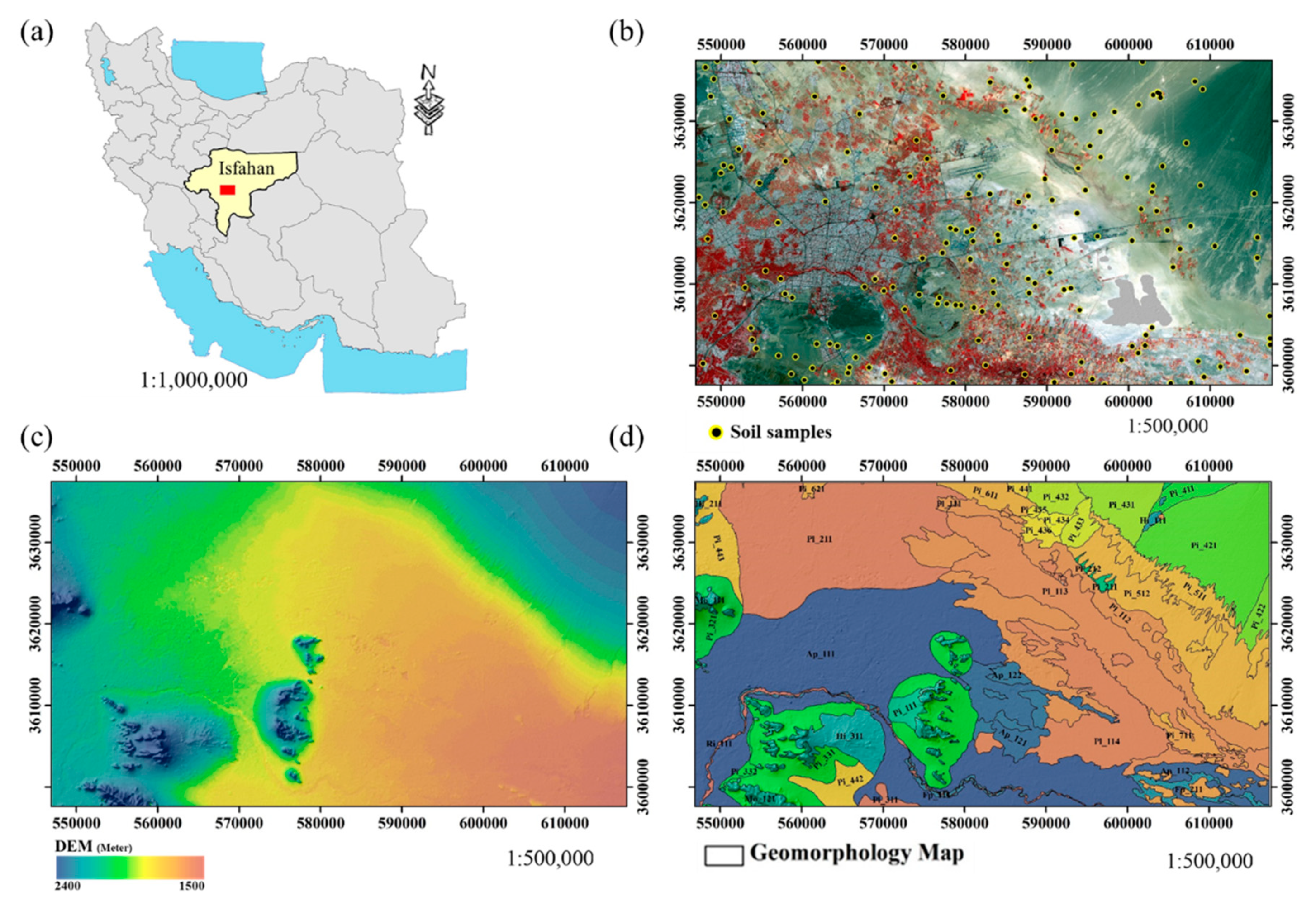
2.1. Study Area

The study area is located in Isfahan, in central Iran (Figure 1a). It covers an area of 150-km² across the Zayandeh-rud basin. Cretaceous limestone, Mesozoic shale and sandstone are the main geologic units in the area. Erosion and deposition are the main geomorphological processes which characterize the area [25]. The mean precipitation, temperature and evapotranspiration in the study area are 110 mm, 14 °C and 1600 mm, respectively. The severity of soil aridity is increasing toward the east of the basin. Interestingly, the elevation generally decreases in this direction.

2.2. Soil Data

The soil sampling strategy was selected to have alignment with the extent of geomorphic surfaces (see Section 2.3.3) and direction of changing slopes. Soil samples were randomly allocated to all delineated geoforms, except the mountains and rocky hills (i.e., stratified simple random sampling) [26]. In total, 194 soil profiles were described [27] with soil samples taken from genetic horizons (Figure 1b). The physico-chemical analyses were measured using Soil Survey Laboratory Methods.

The soil was classified into two Orders: Entisols (43) and Aridisols (151). The former was mainly found in the mountains, hills and colluvial areas and the latter characterizing the predominantly alluvial fans, plateau, playas, flood and river alluvial plains. As shown in

Table 1. Soil types observed in the study area.

Order	No.	Sub-Order	No.	Great Group	No.	Subgroup	No.
Entisols	43	Orthents	43	Torriorthents	43	Typic Torriorthents	43
Aridisols	151	Salids	49	Haplosalids	49	Typic Haplosalids	17
						Gypsic Haplosalids	32
		Argids	34	Haploargids	19	Typic Haploargids	19
				Calciargids	15	Typic Calciargids	15
				Haplogypsids	31	Typic Haplogypsids	24
		Gypsids	44	Calcigypsids	13	Lithic Haplogypsids	7
						Typic Calcigypsids	13
		Calcids	24	Haplocalcids	24	Typic Haplocalcids	24

, the soil profiles in the Entisols Order were classified into the same Sub-order (Orthents), Great Group (Torriothents) and Subgroup (Typic). The soil profiles in the Aridisols were more variable, with most classified into various Sub-orders, including; Salids (49), then Gypsids (44), Argids (34) and Calcids (24). These were then further classified into six Great groups (e.g., Haplosalids) and eight subgroups.

Laboratory analysis of soil samples identified that samples related to zones with saline soils had high values of lime and gypsum content. This is consistent with the fact that the main Sub-orders were the Salids, Argids, Gypsids and Caclids. The organic matter content in the soil was negligible, which is a consistent for soil in arid landscapes. Soil textural classes were highly variable across the study area. Soils developed on highlands were coarser compared with the soil developed on the lower regions such as the output areas of the basin.

2.3. Environmental Variables

The environmental variables which represent the SCORPAN factors are usually derived from a digital elevation model (DEM), remote and proximal sensed data, climatic data, land use, geology and geomorphology maps. Here, 23 environmental variables were derived from a DEM [28,29], remotely sensed satellite data [30,31] and a geomorphology map [26] (

Table 2. Environmental variables used as soil formation factors in the study area.

Definition	Code
Topographic attributes
Slope	SLOPE
Aspect	ASPECT
LS factor	LS
Elevation	Elev
Catchments area	CaA
Catchment network base level	CNBL
Topographic Wetness Index	TWI
Altitude above channel network	AaCN
Multi-resolution Valley Bottom Flatness Index	MrVBF
Multi-resolution of ridge top flatness index	MrRTF
Remote sensing attributes
Clay Index: (shortwave IR-1/shortwave IR-2)	Clay.In
Blue, green, red, near infrared, shortwave IR-1, shortwave IR-2,	Lan.B1-B7
Normalized Difference Vegetation Index: (Shortwave IR-1—Near infrared)/(Shortwave IR-1+ Near infrared)	NDVI
Salinity Index: (Red—Near infrared)/(Red + Near infrared)	Salinity.In
Sentinel Bands 1, 2, 3, and 4	Sen.B1-B4
Geomorphology map
Hierarchical four level classification (geomorphic surfaces)	GEO

). We describe each of these in turn.

2.3.1. Digital Elevation Model

Terrain attributes generally characterise water flow, surface runoff, erosion and deposition rates. The movement and accumulation of water and sediments significantly affects soil forming factors and processes, and thereby the spatial distribution of soil taxonomic classes. Therefore, we used several terrain attributes which are shown in Table 2 derived from a DEM with 30 × 30 m cell size (Figure 1c) [28]. All terrain attributes were computed using SAGA v.2.0.4 (System for Automated Geoscientific Analysis) [29].

2.3.2. Remotely Sensed Optical Satellite Data

In addition to terrain attributes, remotely sensed images are well-known sources of environmental variables which are widely used for prediction [32]. This is because different soil types show different spectral behavior, which can be detected by remote sensors [33]. Spectral bands and their related indices can also be used to approximate vegetation type and land cover and as a soil forming factor. Here, spectral bands of Landsat 8 OLI (operational land imager) and their associated indices (Table 2) were used as covariates to predict USDA soil taxonomic classes in four categories [31]. Moreover, Sentinel Bands including; band 1, 2, 3, and 4, were also used as environmental covariates [30]. The RS-based auxiliary data were derived and calculated based on the median values of cloud-free images taken during 2016.

2.3.3. Geomorphology Map

Geomorphic patterns based on their formation processes, general structure and morphometry were differentiated by air photo interpretation (Figure 1d; See Supplementary Materials). The patterns were described through a nested geomorphic hierarchy. The terminology of legend interpretation was based on [34].

The geomorphic hierarchy classifies geologic, geomorphic and pedogenic processes, and forms in a nested manner. Such a categorical hierarchy was used to decompose the complexity of system and downscale the processes from regional scale to geomorphic surface level. In the lower category, the geomorphic surfaces are considered to be a unit, which have been formed by a specific process in past geologic times. The underlying principle in such a differentiation method is to find edges, dissimilarities or discontinuities of formation processes of adjacent areas and put them into subgroups that are internally as homogenous as possible.

Air photo interpreted delineations of air photos were imported into the ArcGIS software and after ortho-photo geo-referencing, geomorphic surfaces were “glued” via on-screen digitization and geomorphic map were produced. They were then field checked and the boundaries were corrected.

2.4. Soil Taxonomic Class Prediction

2.4.1. Traditional Models

Multinomial Logistic Regression (MnLR)

In cases where the response variable is categorical, logistic regression (LR), which is a simple extension of linear regression, could be employed for prediction. In cases of only two possible outcomes for the dependent variable (e.g., absence of presence of a soil horizon), LR is called a binary LR [35]. When the dependent variable takes more than two possible categories (e.g., USDA soil taxonomic classes presented in Table 1), a simple generalization of binary LR known as Multinomial logistic regression (MnLR) is used for prediction. MnLR uses maximum likelihood to model the probabilities of the possible outcomes of a multi-class dependent variable as a linear combination of a given set of explanatory variables (e.g., environmental variables presented in Table 2).

Artificial Neural Networks (ANN)

ANNs are sophisticated ML algorithms, which are used for both regression and classification in a wide variety of applications. Their capability to reveal non-linear and complex patterns in data are inspired by biological nervous systems, especially of the human brain [35]. The most commonly used ANN structure is multi-layer perceptron (MLP). MLP is a nonparametric approach that can be used for both classification and regression [35]. Neurons are usually organized in three layers: input, hidden and output layers. Data are introduced to the network through the input layer and processed by the hidden layer to produce the outputs. Here, we used a MLP network with sigmoid and linear activation functions in the hidden and output layers, respectively. Also, a back-propagation algorithm based on the Levenberg–Marquardt least-squares minimization [36] was used to train the network. The created network was trained by soil taxonomic classes as target variable, and the environmental variables as predictor.

Support Vector Machines (SVMs)

SVMs are used for regression and classification. The algorithms were initially developed by Vapnik [37] to find hyperplanes to classify linearly separable classes of objects. In most real-world applications, classes of objects cannot be separated linearly. To overcome the problem, the input data could be transformed into a higher dimension space using a nonlinear function [38]. This transformation is often done using a kernel function. Kernels are mathematical functions that transform the data in a higher dimension space in which the data could become more easily separated [38].

Maximum margin solution is used by SVMs to choose the hyperplanes providing the minimum error, whereby the larger the margin, the higher the generalization ability of the classifier. The data that are nearest to the maximum margin of a hyperplane are known as support vectors. Because of the ability of the radial basis function (RBF) introduced by Hsu et al. [39] in acting as a universal function approximator, it was used as the kernel function in this study. Also, to optimize the parameters of the SVM, we used a simulated annealing algorithm.

Decision Tree (DT)

Decision Trees (DT) are hierarchical and nonparametric models that are commonly used for both classification and regression. They have the ability to learn and respond quickly as well as high performance in a wide range of applications [40]. Also, the IF-THEN rules that the decisions are based on, can be understood and validated by experts [35]. In the case of the supervised learning algorithm, the hierarchical structure of the tree is created by using a divide-and-conquer algorithm [35]. Through the algorithm, a main complex problem is partitioned into two or more simple sub-problems in a sequence of recursive splits. Partitioning will be stopped when the sub-problems become simple enough to be solved. Eventually, the main problem is solved by combining the solved sub-problems.

A classification process begins at the root node and it is then introduced to the internal decision nodes in the hierarchy of a DT. Based on the outcome of a test function which is implemented on the attributes of classification, choices are made in decision nodes. According to the choices, the data are divided into several branches that represent potential outcomes of a decision. The process is repeated recursively until the branches do not split anymore and the tree is ended in the leaf nodes, points that the expected outcomes are obtained. Here we used a decision tree (DT) algorithm as a classifier to model the relationship between soil taxonomic classes and environmental variables.

Random Forest (RF)

A Random Forest (RF) involves an ensemble of decision trees via a bootstrap method which is used as a learning algorithm for a predictive model [41]. In the bootstrap aggregating (bagging) approach, the variance is reduced by averaging many tree-based models. The approach involves random selection of the subsamples of the given data via mtry parameter which they are combined based on the tree-structured classifiers [42]. Each tree grown in the forest is associated with the values of a random vector which is not dependent on the other random vectors but with the same distribution. The generated random vectors of explanatory variables and a training dataset are used to build a classifier. During the classification process, many trees (ntree) are generated. All trees are voted, with the tree receiving the most votes in the forest, selected as the final prediction of the given variable. Examples of recent applications of RF in DSM include those in citation [43]. Herein, we optimized two parameters (mtry and ntree), by iterating mtry values from 2 to 23 and ntree values from 100 to 10,000.

Bayesian Networks (BN)

In cases of partial information and the probability distribution of input data, the Bayesian networks (BN) can work efficiently [44,45]. Some studies have explored the use of BN in predicting soil classes [46].

BN are probabilistic graphical structures that represent a set of random variables and the associated conditional correlations, using a directed acyclic graph (DAG). In a DAG, the nodes and links indicated random variables and direct connection between them, respectively. The relationships between cause and effect in BNs are shown through the connections [46]. Unlike deterministic models, BN is a flexible approach to deal with the random processes and can reveal the uncertainty in cause-effect relationships [46].

Unlike other network-based models (e.g., ANNs), in BNs, the user, by considering the main process underlain, can define the network and the interactions between the nodes. In terms of DSM, a BN could represent the probabilistic relationships between soil taxonomic class data and auxiliary variables, hence the probabilities of the presence of soil taxonomic classes could be predicted by a BN [46,47].

The most important issue in the design of BNs is the type of learning procedure. There are two learning processes for BN, including parametric and structural. The structural learning can determine the optimum structure in BN. The limit-oriented and point-oriented techniques are the two most commonly used for classification in a structural learning process. The base of a limit-oriented technique in a learning process is the establishment of autonomous connection among the nodes in networks [47].

Five different point-oriented ways and one limit-oriented way were applied in the learning stage of the present study. The genetic, hill climber, K2, simulated annealing and Tabu search were five point-oriented approaches used herein. A conditionally independent search was only used and represents the only limit-oriented approach to run the learning stage of BNs.

Sparse Multinomial Logistic Regression (SMnLR)

Sparseness has been introduced as an approach to enhance the generalization capabilities of the Multinomial Logistic classifiers. Learning algorithms, which are employed in sparse classifiers, are among the state-of-the-art in supervised learning methods [48]. A learned classifier can improve its generalization capacity by minimizing the number of basis functions. To learn a classifier as sparsely as possible, some preceding belief are typically supposed to regulate the likelihood of the weights of training data [38]. These prior beliefs help to promote the sparsity of weights.

Sparse multinomial logistic regression (SMnLR) is an accurate and sophisticated method that provides a sparse solution for prediction of categorical variables. It also provides explicit information on the probabilities of classification without knowing the exact information about the class. SMnLR is a multi-category classifier that is trained by a training data set. By adapting a Laplacian prior, SMnLR performs variable selection to determine a subset of the most relevant predictors. Although SMnLR has been used mostly in biological studies by Hartemink [49], but a little attention paid in DSM study as lamented by Hartemink [23].

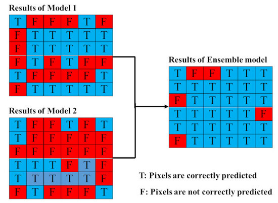
2.4.2. Proposed Ensemble Models

Two general techniques have been used for ensemble of prediction of continuous variables. The first is the variance-weighted method [50], where the ensemble is an average of all models, where each model is weighted by the variance of prediction. The second is known as the Granger-Ramanathan method [51]. However, ensemble method for digital soil class prediction has not been well explored.

Here, we combined prediction of seven data mining models to explore how much the suggested ensemble approach could improve the final predicted soil classes. For categorical variables, we modified the above two ensemble methods as follows. The majority method, which follows the Random Forest method, is where the ensemble selects the most frequently predicted soil class by the different models (Ensemble.1). A multinomial regression method, which relates all models as predictors to observed soil classes (Ensemble.2). This involves fitting a multinomial regression between predictions from different models and observed values from the training data. The ensemble model can be written as:

$$P\left(A\right)=\frac{\exp \left({\mathsf{\beta }}_0+{\mathsf{\beta }}_{A1}\mathrm{MnLR}+{\mathsf{\beta }}_{A2}\mathrm{ANN}+{\mathsf{\beta }}_{A3}\mathrm{SVM}+{\mathsf{\beta }}_{A4}\mathrm{DT}+{\mathsf{\beta }}_{A5}\mathrm{RF}+{\mathsf{\beta }}_{A6}\mathrm{BN}+{\mathsf{\beta }}_{A7}\mathrm{SMnLR}\right)}{\exp \left({\mathsf{\beta }}_0+{\mathsf{\beta }}_{A1}\mathrm{MnLR}+{\mathsf{\beta }}_{A2}\mathrm{ANN}+{\mathsf{\beta }}_{A3}\mathrm{SVM}+{\mathsf{\beta }}_{A4}\mathrm{DT}+{\mathsf{\beta }}_{A5}\mathrm{RF}+{\mathsf{\beta }}_{A6}\mathrm{BN}+{\mathsf{\beta }}_{A7}\mathrm{SMnLR}+\cdots +{\mathsf{\beta }}_0+{\mathsf{\beta }}_{L1}\mathrm{MnLR}+{\mathsf{\beta }}_{L2}\mathrm{ANN}+{\mathsf{\beta }}_{L3}\mathrm{SVM}+{\mathsf{\beta }}_{L4}\mathrm{DT}+{\mathsf{\beta }}_{L5}\mathrm{RF}+{\mathsf{\beta }}_{L6}\mathrm{BN}+{\mathsf{\beta }}_{L7}\mathrm{SMnLR}\right)}$$

(1)

where P(A) is the probabilities of occurrence class (A) (e.g., Typic Torriorthents), β₀ is a constant, β_A1 to β_A7 is regression coefficients, and MnLR, ANN, SVM, DT, RF, BN and SMnLR are explanatory variables. The output used in this study is the most probable class.

2.5. Validation

Validation criteria used to assess the DSM prediction were the overall accuracy (OA) and Cohen’s kappa coefficient index (κ). OA is calculated as the percentage of correctly predicted class, while κ measures inter-rater agreement for categorical variables. These criteria were calculated from a 10-fold-cross validation with 100 repeats at four soil taxonomic levels. Furthermore, we used some validation criteria which show the true and false prediction of soil class taxa at subgroup level. For each prediction models at subgroup level, the true positives of presence and the false positives of absence were determined by sensitivity (Se) and specificity (Sp), respectively. Additionally, the area under the curve (AUC) was calculated for all soil taxonomy levels. The AUC is estimated by numerical integration as a measure of the overall quality of the map.

3. Results and Discussion

3.1. Soil Taxonomic Class Prediction

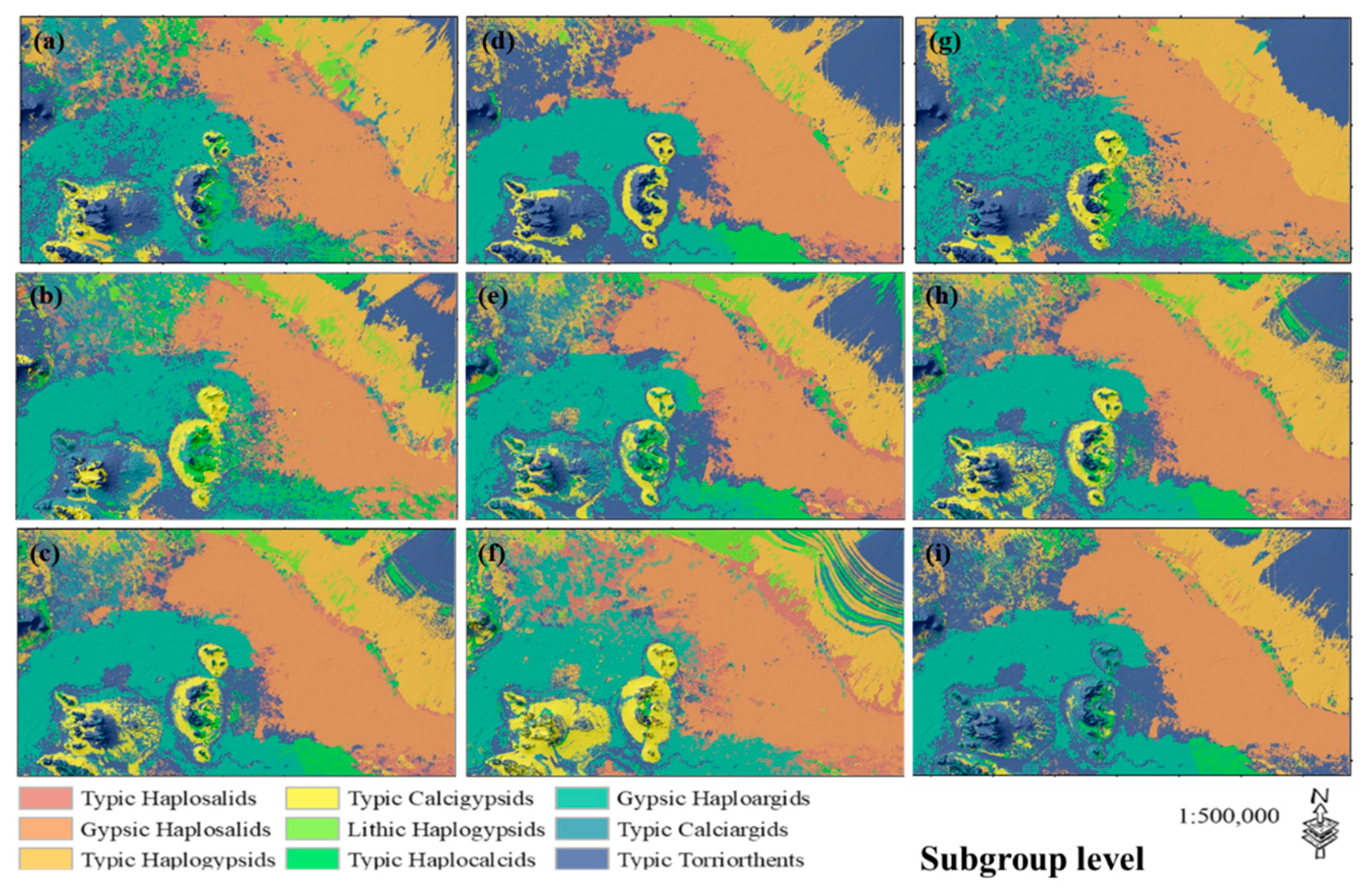
3.1.1. Traditional Models

Multinomial Logistic Regression (MnLR)

The MnLR was performed using the main soil taxonomic classes (target) and environmental (predictor) variables (DEM, remote sensed satellite data and geomorphology map). The statistical results showed that the fitted regression model was significant at the 1% level of probability. The results of overall accuracy (OA) and AUC of the MnLR modeling was largest at the Order (0.64 and 0.66) level (

Table 3. Validation criteria of all models to predict soil taxonomy classes. Values highlighted in bold represent results with the largest accuracy.

Methods	Models	Order			Sub-Order			Great Group			Subgroup
		OA	κ	AUC	OA	κ	AUC	OA	κ	AUC	OA	κ	AUC
Traditional models	MnLR	0.64	0.23	0.66	0.40	0.25	0.46	0.34	0.22	0.49	0.34	0.24	0.48
	ANN	0.81	0.41	0.71	0.51	0.37	0.57	0.48	0.36	0.66	0.39	0.28	0.56
	SVM	0.86	0.51	0.71	0.44	0.27	0.54	0.41	0.23	0.52	0.37	0.22	0.42
	DT	0.81	0.46	0.73	0.42	0.26	0.53	0.45	0.34	0.65	0.37	0.27	0.53
	RF	0.87	0.57	0.75	0.52	0.38	0.60	0.46	0.34	0.65	0.41	0.30	0.64
	BN	0.79	0.41	0.68	0.47	0.33	0.57	0.42	0.30	0.62	0.40	0.30	0.64
	SMnLR	0.86	0.51	0.71	0.51	0.37	0.59	0.45	0.31	0.57	0.37	0.23	0.42
Ensemble models	Ensemble.1	0.86	0.54	0.74	0.50	0.36	0.60	0.46	0.33	0.66	0.39	0.27	0.61
	Ensemble.2	0.90	0.66	0.81	0.70	0.61	0.73	0.61	0.52	0.69	0.53	0.43	0.67
	RI (%) *	3.4	15.8	7.4	34.6	60.5	17.8	27.1	44.4	4.5	29.3	43.3	4.6

MnLR: Multinomial Logistic Regression; ANN: Artificial Neural Networks; BN: Bayesian Networks; SVM: Support Vector Machines; RF: Random Forest; DT: Decision Tree; SMnLR: Sparse Multinomial Logistic Regression; OA: Overall Accuracy; AUC: area under curve. * RI: Relative improvement of accuracy, Kappa index and AUC of Ensemble.2 Method compared with the most accurate prediction.

). However, the OA fell away sharply at the Sub-order (0.40), Great group (0.34) and subgroup (0.34) levels (Table 3), but AUC values almost were constant for Sub-order (0.46), Great group (0.49) and subgroup (0.48) levels (Table 3).

In terms of the Kappa statistic, the results for the MnLR were a little more revealing in terms of inter-rater reliability at the different levels of the Soil taxonomy. The most reliable classification occurred at the Order level (κ = 0.23) which showed above the fair agreement (0.21–0.40). A fair agreement was also achieved at the Sub-order (0.25), Great group (0.22), and Subgroup (0.24) levels.

Table 4. Sensitivity analysis of different models to predict soil classes at the Subgroup level.

Methods	Methods		GHS	LHG	TCA	TCG	THA	THC	THG	THS	TTO
Traditional models	MnLR	Se	0.66	0.29	0.40	0.00	0.68	0.17	0.33	0.29	0.16
		Sp	0.88	0.95	0.88	0.97	0.89	0.94	0.92	0.97	0.85
		PPV	0.51	0.17	0.22	0.00	0.39	0.29	0.38	0.45	0.23
	ANN	Se	0.69	0.14	0.20	0.38	0.21	0.25	0.38	0.18	0.53
		Sp	0.88	0.99	0.94	0.97	0.97	0.93	0.89	0.97	0.73
		PPV	0.54	0.33	0.23	0.45	0.40	0.35	0.33	0.38	0.36
	SVM	Se	0.72	0.14	0.00	0.08	0.21	0.17	0.12	0.06	0.81
		Sp	0.78	0.99	0.99	1.00	1.00	1.00	0.98	0.98	0.49
		PPV	0.40	0.50	0.00	1.00	1.00	1.00	0.43	0.20	0.31
	DT	Se	0.62	0.00	0.27	0.46	0.32	0.29	0.33	0.23	0.39
		Sp	0.88	0.97	0.96	0.94	0.91	0.92	0.92	0.95	0.81
		PPV	0.51	0.00	0.36	0.35	0.27	0.33	0.38	0.33	0.38
	RF	Se	0.75	0.00	0.27	0.38	0.16	0.21	0.42	0.23	0.56
		Sp	0.89	0.99	0.95	0.97	0.96	0.93	0.90	0.97	0.97
		PPV	0.57	0.00	0.33	0.50	0.30	0.29	0.37	0.44	0.44
	BN	Se	0.75	0.00	0.27	0.00	0.00	0.08	0.42	0.06	0.06
		Sp	0.88	0.99	0.97	0.99	0.99	0.96	0.89	0.99	0.99
		PPV	0.54	0.00	0.44	0.00	0.00	0.22	0.36	0.33	0.33
	SMnLR	Se	0.50	0.00	0.33	0.31	0.16	0.46	0.54	0.29	0.29
		Sp	0.96	0.98	0.94	0.94	0.96	0.86	0.89	0.94	0.94
		PPV	0.73	0.00	0.31	0.27	0.30	0.32	0.42	0.33	0.33
Ensemble models	Ensemble.1	Se	0.72	0.00	0.27	0.31	0.16	0.17	0.37	0.18	0.18
		Sp	0.87	0.99	0.97	0.96	0.97	0.95	0.90	0.98	0.98
		PPV	0.52	0.00	0.40	0.40	0.37	0.33	0.35	0.43	0.43
	Ensemble.2	Se	0.69	0.29	0.13	0.23	0.47	0.50	0.50	0.23	0.23
		Sp	0.95	0.99	0.96	0.99	0.95	0.96	0.97	0.99	0.99
		PPV	0.73	0.50	0.22	0.75	0.53	0.63	0.75	0.67	0.67

GHS: Gypsic Haplosalids; LHG: Lithic Haplogypsids; TCA: Typic Calciargids; TCG: Typic Calcigypsids; THA: Typic Haploargids; THC: Typic Haplocalcids; THG: Typic Haplogypsids; THS: Typic Haplosalids; TTO: Typic Torriorthents; MnLR: Multinomial Logistic Regression; ANN: Artificial Neural Networks; SVM: Support Vector Machines; DT: Decision Tree; RF: Random Forest; BN: Bayesian Networks; SMnLR: Sparse Multinomial Logistic Regression; Se: sensitivity; Sp: specificity; PPV: users’ accuracy or positive predicted values.

shows the sensitivity analysis of the MnLR to predict soil taxonomic classes at the Subgroup level indicated that the best results regarding sensitivity (Se) by the MnLR model for all studied Subgroups were for the Typic Haploargids (0.68) (Table 4). The next best was the Gypsic Haplosalids (0.66) and Typic Calciargids (0.40) of the Aridisols Order. By contrast, the worst sensitivity was obtained for Typic Calcigypsids (0.00), Typic Torriorthents (0.16) and Typic Haplocalcids (0.17). Equivalent rankings with respect to the Positive Predicted Value (PPV) were evident, with the largest being for the Gypsic Haplosalids (0.51) and smallest for Typic Calciargids (0.00). The results achieved herein for the MnLR model were satisfactory and consistent, more or less, with those reported by several other researchers [4,52].

Artificial Neural Networks (ANN)

Table 3 shows that the OA and AUC of the ANN for prediction of the different soil taxonomic classes again decreased in sequence from the Order (0.81 and 0.71) level which was largest, with Sub-order (0.51 and 0.57) and Great group (0.48 and 0.66) intermediate and Subgroup (0.39 and 0.56) smallest. The slightly larger OA results for the ANN method at all levels, and in comparison to the MnLR model, indicates that ANN had greater accuracy.

This was reinforced with a slightly larger κ statistic. The largest was achieved at the Order (0.41) level, which indicates moderate agreement (0.41–0.6), with Sub-order (0.37), Great group (0.36), and Subgroup (0.28) showing fair agreement. The results showed that using 9 hidden neurons and 200 epochs were the best combination for predicting subgroups. Therefore, the structure of 23-9-9 is proper to predict soil classes at the Great group level.

Furthermore, the results of the confusion matrix for the training stage indicated that the largest sensitivity (Se) was achieved for the Gypsic Haplosalids (0.69), Typic Calcigypsids, and Typic Haplogypsids (0.38) (Table 4). Conversely, the smallest were for the Lithic Haplogypsids (0.14) and Typic Haplosalids (0.18). These results could be due to the small numbers of observational data [4,15,24]. However, these results were equivalent to those achieved by several other researchers [14,15], who predicted the soil units using ANNs and environmental variables, such as slope, elevation, solar radiation, geology and geomorphology maps.

Super Vector Machine (SVM)

Modeling soil taxonomic classes by SVM algorithm was performed based on the selected function (kernel function of RBF). Three parameters of kernel function (i.e., parameter, insensitive parameter and punishment coefficient) were optimized using the simulated annealing algorithm. For Subgroup level modeling, optimized values were 0.5, 0.04 and 28, respectively.

Table 3 shows that the OA of the SVM, except for Order level, decreased in accord with the ANN results, with Order (0.86) largest, with Sub-order (0.44) and Great group (0.41) intermediate. With respect to the OA for Sub-order and Great group, these were larger than those for the equivalent levels of MnLR. The Subgroup OA (0.37) was again the smallest and smaller than ANN. Also, AUC of SVM approach decreased from Order to Subgroup levels. The largest and smallest values of ACU were observed for Order (0.71) and Subgroup (0.42) levels, respectively (Table 3). This suggests an acceptable performance for Order level.

Furthermore, the largest and smallest values of the κ statistic were observed for Order (0.51) and subgroup (0.22) levels, respectively (Table 3). This suggests moderate agreement and superior again in comparison to the results achieved with respect to MnLR for Order, Sub-order, and Great group levels.

Table 4 shows that the best sensitivity was related to Typic Torriorthents (0.81) and Gypsic Haplosalids (0.72) with PPV the largest for Typic Calcigypsids, Typic Haploargids, and Typic Haplocalcids (1.00) (Table 4). The worst sensitivity and positive predicted value was for the Typic Calciargids (0.00). High performance of the SVM method for prediction of soil classes has been reported in several studies [10,15]. The higher performance of SVM (radial basis function) in comparison with several ML algorithms (kNN, MnLR, ANN and RF techniques) was reported by [10] in order to predict the Great group and Order levels of soil taxonomy.

Decision Tree (DT)

A DT uses a series of logical terms in the form of an algorithm, which has the structure of a tree. We used this approach here to classify the soil taxonomic classes. The results showed that the OA of the DT for the prediction of soil taxonomic classes at Order level was small (0.81) compared to SMnLR (86%), RF (0.87) and SVM (0.86), but the AUC values for DT was larger (0.73) than those except for RF approach. Nevertheless, the OA values again decreased in rank order from Sub-order (0.42), Great group (0.45) and Subgroup (0.37) levels. The AUC values also decreased from Order to Subgroup levels from 0.73 to 0.53, respectively.

As with the previous three methods, the largest κ statistic values were observed for Order (0.46) and Great group (0.34) levels (Table 3), which indicate moderate agreement; superior to MnLR and almost equivalent to the results achieved for ANN for both levels.

The maximum sensitivity and PPV belonged to the Gypsic Haplosalids (0.62 and 0.51, respectively) (Table 4). The minimum sensitivity and PPV of classification was also related to Lithic Haplogypsids (0.00) and Typic Haplocalcids. Various studies confirmed the efficiency of the DT model to predict soil classes [12,15].

Random Forest (RF)

The OA and AUC results for the RF were almost equivalent to SMnLR and SVM (0.87 and 0.75) at the Order level but fell away as sharply as those for the SMnLR and SVM method but were still slightly larger. The RF method returned the largest κ statistics at the Order (0.57) and Sub-order (0.38) levels and among all individual models. The estimation error of OOB (out-of-bag error) was 55% at soil family level that was also previously reported by [53] when RF was used to classify 672 soil profiles. Moreover, Brungard et al. [3] and Pahlavan-Rad et al. [5] obtained estimation errors of 53% and 45%, respectively, when RF was used to predict soil taxonomic classes. The maximum sensitivity and positive predicted value were for Gypsic Haplosalids, whereas, the worst was for the Lithic Haplogypsids (Table 4).

Bayesian Networks (BN)

The OA for the BN approach, like other methods, indicated decreasing trend from the Order to Subgroup levels. The largest and smallest OA obtained was for the Order (0.79) and Subgroup (0.40), respectively. The AUC values decrease from Order to Sub-order levels (0.68 to 057), but this validation index did not show same trend form Sub-order to Subgroup levels for BN approach. The κ was the largest for Order (0.41) and smallest for Great group and Subgroup (0.30) levels. Generally speaking, at the level of Order which was largest of any level, the k statistic was larger than the MnLR (0.40) (Table 3).

The maximum sensitivity belonged to Typic Haplogypsids (0.54), with the largest PPV belonging to Typic Haplogypsids (0.42) and Typic Torriorthents (0.42) (Table 4). The smallest sensitivity (0.00) and PPV (0.00) of classification was also related to the soil class of Lithic Haplogypsids.

Sparse Multinomial Logistic Regression (SMnLR)

The SMnLR approach showed the most promising performance compared to the other methods. This method has been developed in genetics and biology data analysis promoted by Hartemink [49], including a Bayesian analysis by Hartemink [44]. Overall accuracy at the Order level was the largest (0.86) among all individual models. While the OA and AUC of SMnLR decreased from Order to Subgroup levels as expected, it was always among the best models (Table 3).

These results were repeated in terms of the κ statistic among all studied models and at the four soil taxonomic levels (Table 3). Also, the best sensitivity (0.75) and PPV (0.54) were obtained for Gypsic Haplosalids (Table 4).

3.1.2. Proposed Ensemble Models

To determine if we could improve the prediction of soil classes at different taxonomic levels (Table 3), we tested two ensemble modeling techniques. The majority method (Ensemble.1) appears not to be able to produce better accuracy when compared to the best single model. However, the increase in accuracy ranged from 3 to 25% when Ensemble.2 model was used. The results showed that the OA of the Ensemble.2 approach of the different soil taxonomic classes were obtained from Order (0.90), Sub-order (0.70) to Great-group (0.61) and Subgroup (0.53). This represents improved accuracy of 3%, 35%, 27%, and 29% (from Order, Sub-order, Great-group and Subgroup). While the accuracy improvement in the Order level is small, as the best model is already accurate (OA RF = 0.87), the improvement at other taxonomic levels is significant as the accuracy of a single best method is still low, e.g., the OA at the Sub-order level for RF = 0.52, while OA of Ensemble.2 = 0.70. Furthermore, AUC values of Ensemble.2 at four levels of soil taxonomy were the largest values among all studied models (Table 3). The results showed an acceptable performance for Sub-order, Great group and Subgroup levels and an excellent performance for Order level [54].

The κ index ranged from 0.43 to 0.66 at Subgroup and Order levels, respectively (Table 3). The results demonstrated that the Ensemble.2 modelling approach produced more accurate and reliable predictive soil taxonomic results than the models individually (i.e., MnLR, ANNs, SVMs, DT, RF, BNs and SMnLR) especially at soil taxonomic levels lower than the Order level. This result is an expected outcome for this type of ensemble modeling method [19,21].

The sensitivity analysis of different methods to predict soil taxonomic classes at the Subgroup level proved that when Ensemble.2 model was applied, the reliability and accuracy of individual soil Subgroup increased (Table 4). The maximum sensitivity at subgroup level belonged to Typic Torriorthents, while and also, the best positive predicted value related to Gypsic Haplosalids, Typic Calcigypsids, and Typic Haplogypsids.

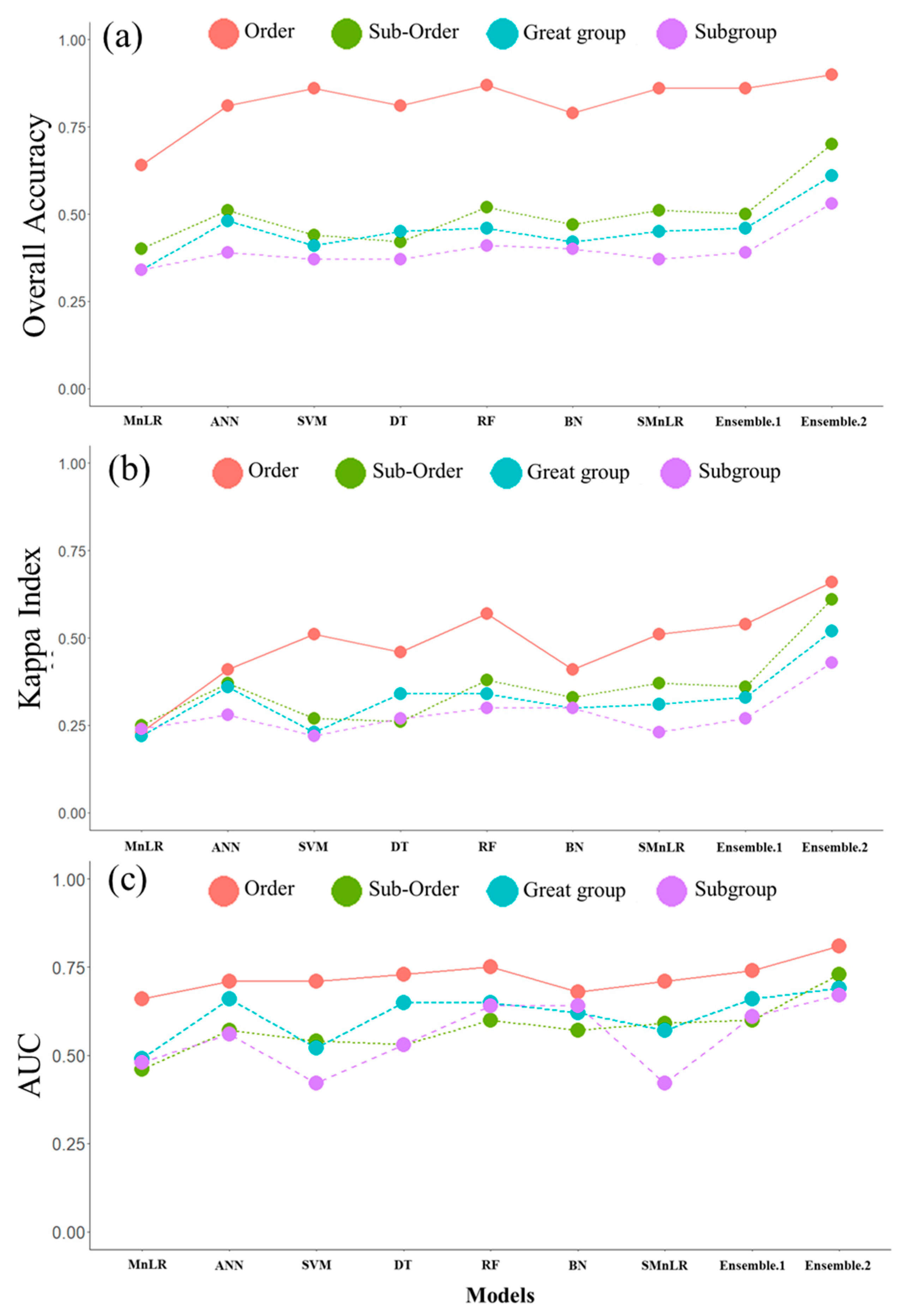
3.1.3. Comparison of Traditional and Ensemble Models

A review of the available literature showed that researchers often employed different methods or models to predict the soil classes depending on the circumstances. Almost all of them stated that each model has its unique performance and has its particular strengths and weaknesses. The results of the present study showed that each specific model was superior in prediction of a specific soil taxonomic class. For example, the RF model had the best prediction for Gypsic Haplosalids (0.75), while the model of MnLR predicted the Typic Haploargids with the highest sensitivity (0.68). In addition, MnLR had the poor performance to predict Lithic Haplogypsids (PPV = 0.17) and Typic Calcigypsids (PPV = 0.00).

These different results and observations are mainly related to the complex nature and distinct mathematics of each model. Furthermore, the sensitivity of each model could be strongly affected by the number of soil samples (see Table 1). For instance, Taghizadeh-Mehrjardi et al. [15] reported that the regression models are strongly correlated with the number of soil samples. Perhaps this issue was the reason of low efficiency of the MnLR for predicting the Lithic Haplogypsids and Typic Calcigypsids.

However, the multinomial ensemble method introduced in this study predicted the soil classes at the subgroup level using the strength of each specific technique in the current study (Table 3). The sensitivity of this combined model for predicting soil classes was more than other models. For example, the combined model could increase the individual accuracy (PPV) of Lithic Haplogypsids (~66%) and Typic Calcigypsids (~100%), compared to the MnLR.

Results also showed that the Ensemble.2 model had more accuracy in term of OA and AUC compared with when the models were used in isolation (Table 3). The suggested ensemble model (Ensemble.2) increased the OA and AUC compared to the best individual model (RF) (Figure 2). The OA increased for the Ensemble.2 model compared to RF model for soil Order (~3%), Sub-order (~25%), Great group (~24%) and Subgroup (~22%) levels, respectively. Also, the AUC values increased for the Ensemble.2 model compared to the RF model for soil Order, Sub-order, Great group and Subgroup levels, respectively, ~8%, 22%, 6%, and 5% (Table 3 and Figure 2).

Similarly, the κ statistic increased for the suggested empirical model compared to the RF model. The ensemble model (Ensemble.2) increased ~13%, ~37%, ~34%, ~30% the kappa index for soil Order, sub-order, Great group and Subgroup levels, respectively (Figure 2b). These results can show the high efficiency of the suggested combined model using multinomial regression (Ensemble.2) for soil classification. The ensemble model is a favorable method if the combined model is more accurate than each individual model [19].

The suggested ensemble model was used to predict other soil taxonomic classes. This stage was necessary to compare the results in other soil taxonomic levels from Order to Sub-order and Great group. As can be seen in Figure 2, the OA, the κ statistic and AUC of all the studied models decreased from Order to Subgroup levels. This result is in accord with other similar works [3,4,6,15].

Moreover, the results showed that the new suggested empirical model increased the power of prediction of the individual soil classes in other soil taxonomic levels similar to the Subgroup level. For example, the positive predicted value of the new combined model (Ensemble.2) was more than MnLR improving at the Great group level, in particular Haplogypsids (~20%) and Calcigypsids (~75%).

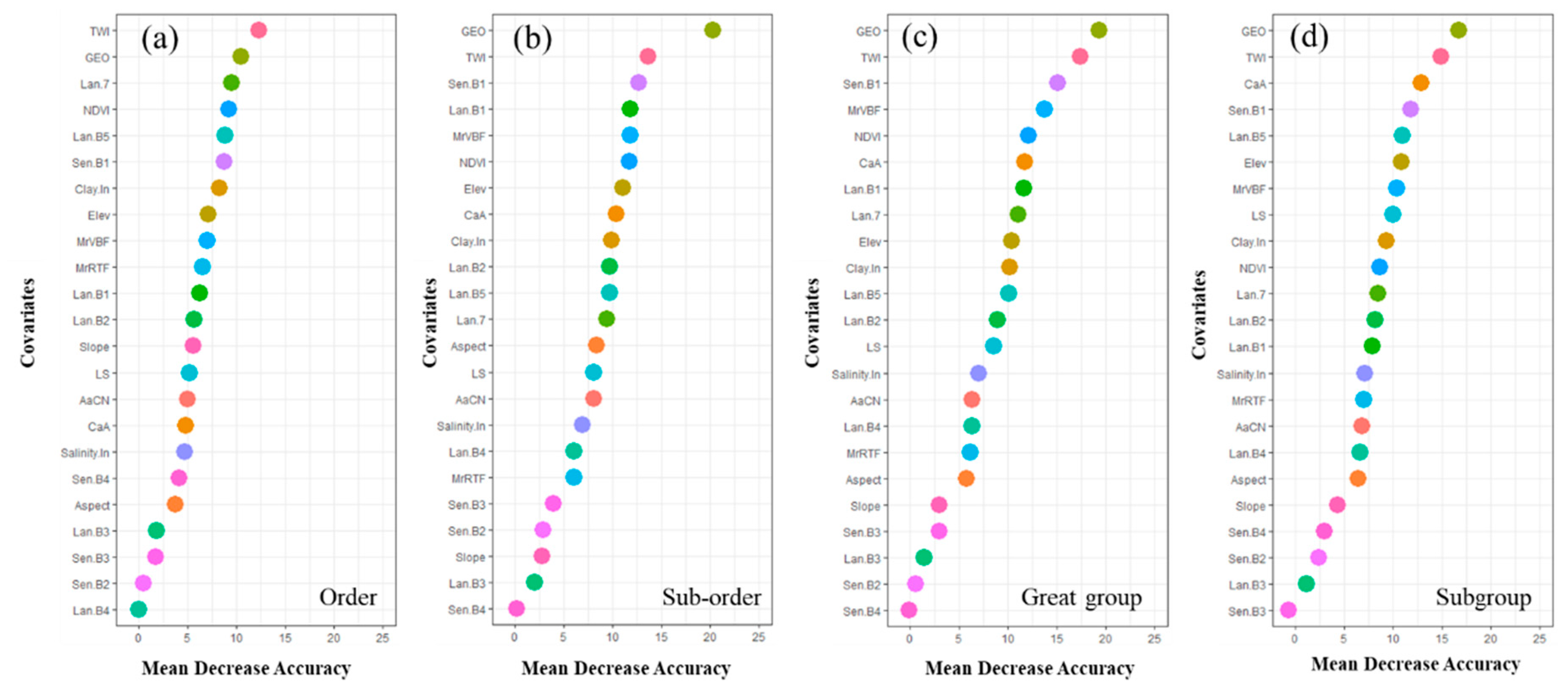
3.2. Environmental Variables

Figure 3 shows the 23 environmental variables used in prediction in order of importance in different taxonomic categories. The most effective variable in all taxa prediction was the Geomorphology map. It highlights strong inherent relationship of this variable with different soil taxon formation and development. These results were consistent with the literature studied in Iran [4,15,24].

It is also worth noting that six of the nine DEM-derived data variables were among the top ten most important variables used in all predictions with the Ensemble.2 method. This highlights the importance of topography in predicting soil classes [2,4]. Among them, Catchments Area (CaA) and Topographic Wetness Index (TWI) confirm the importance of moisture status and hydrology within soil differentiation of arid regions [4,15,24].

The first three variables, which have the most effective role in soil Subgroup predictions, rely on the remotely sensed satellite images, specifically the environmental variables of Sentinel Radar Band 1 and Landsat 8 OLI (operational land imager) short wave band. These are important because they represent chemical weathering and soil evolution. Overall, the first nine variables, with some variation up and down, were the same covariates with high importance within prediction processes of all soil taxa (Figure 3).

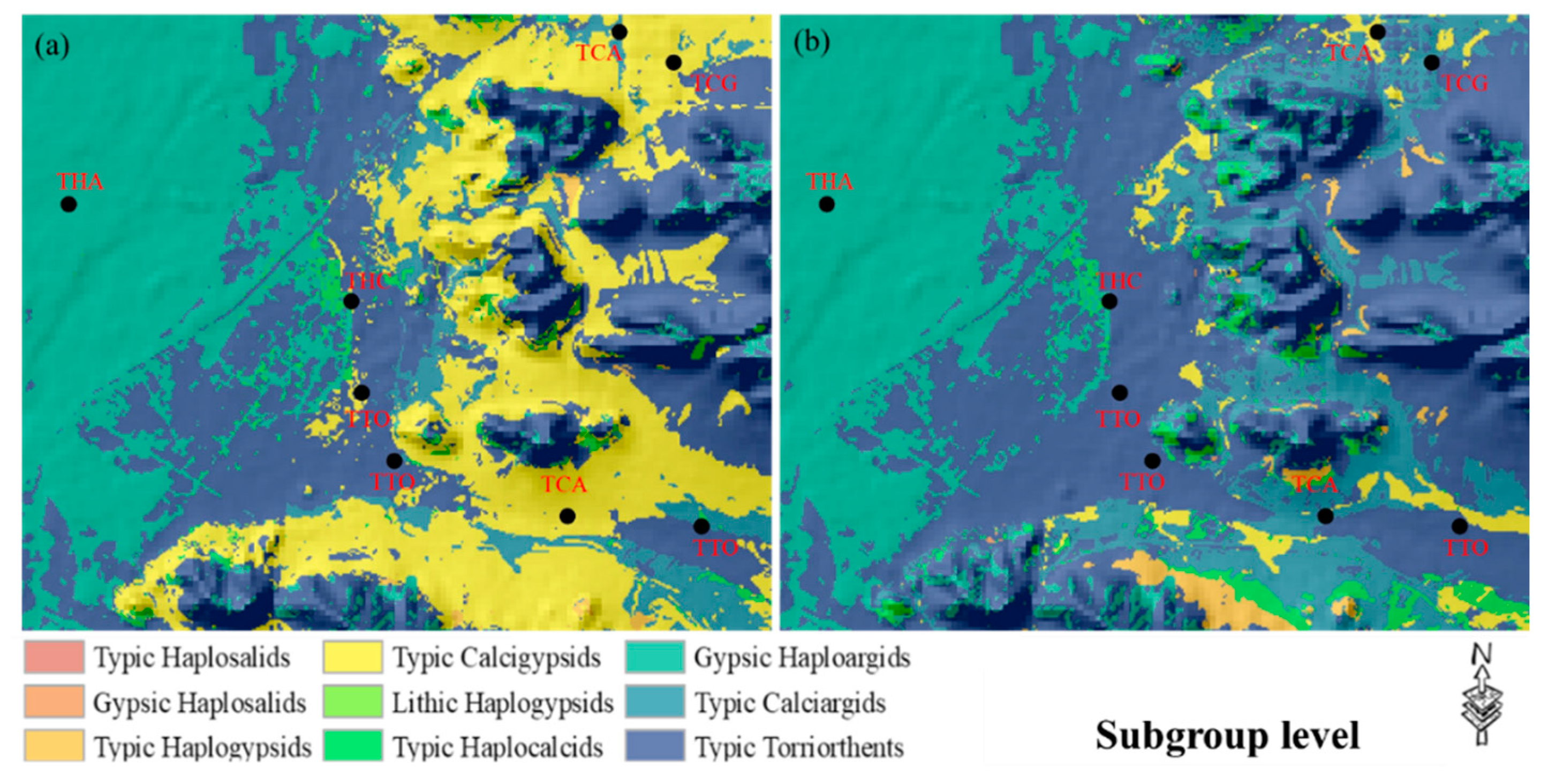
3.3. Spatial Prediction of Soil Classes Using Suggested Ensemble Method

Here, we presented different approaches to digitally map soil classes in Isfahan province. Figure 4 shows the predicted spatial distribution of soil classes at the Subgroup level for different approaches. The validation procedures prove that the best prediction result was obtained by the Ensemble.2 model. It was completely visible considering the calculated OA out of that approach in Order (0.90), Sub-order (0.70) to Great group (0.61) and Subgroup (0.53) taxonomic category levels.

Despite of the high κ statistic and AUC, overall the map (Figure 4i) from this approach looks promising. This was because it coincides with our understanding of the spatial distribution of soil classes across the study area, and as determined by the various SCORPAN factors, in particular, climate, parent material, biotic and human impacts on soil formation.

The area of study was characterized by some calcareous mountains (Cretaceous over Jurassic sediments) with its proportional piedmonts; river alluvial plains, gravelly plateaus and playas. Nevertheless, in the prevailing arid climate, the area had some different influential paleoclimatical epochs, resulting in completely different evolutional unconformities for different geomorphic geoforms of the Zayandeh rud basin.

The paleoclimatic conditions developed various combinations of argillic, calcic and sparsely gypsic horizons in soils developed on stable piedmonts resulting in Haplo or Calciargids. These were shown to be better predicted than the other methods (see Figure 4i). The soils developed on river terraces, formed argillic horizons, morphing to cambic and ochric horizons from the first to third river terraces, respectively depending on surface stability. This confirms the accuracy of Haploargids and Calciargids distribution in these terraces.

Playa soils were characterized mostly by salic combined with some gypsic horizons confirming the predicted Typic or Gypsic Haplosalids in these landscapes. The soils developed on plateaus were mainly composed of gravelly gypsiferous materials, which were concordant with predicted Calcic or Haplogypsid classes in these landforms. Entisols which developed on recently deposited sediments everywhere under current climatic condition seem promising in different geoforms.

In addition, we did a zoom in to a smaller area (Figure 5), to explore the differences between two maps generated by an individual model (i.e., RF) and Ensemble model (i.e., Ensemble2). As can be seen, the general spatial distribution of soil classes is fairly similar. However, there are some differences, in particular, the soils predicted as Typic Calciargisds and Typic Calcigypsids. When the predicted soil classes compared with actual soil profiles, we could conclude that Ensemble.2 model was much more successful in DSM.

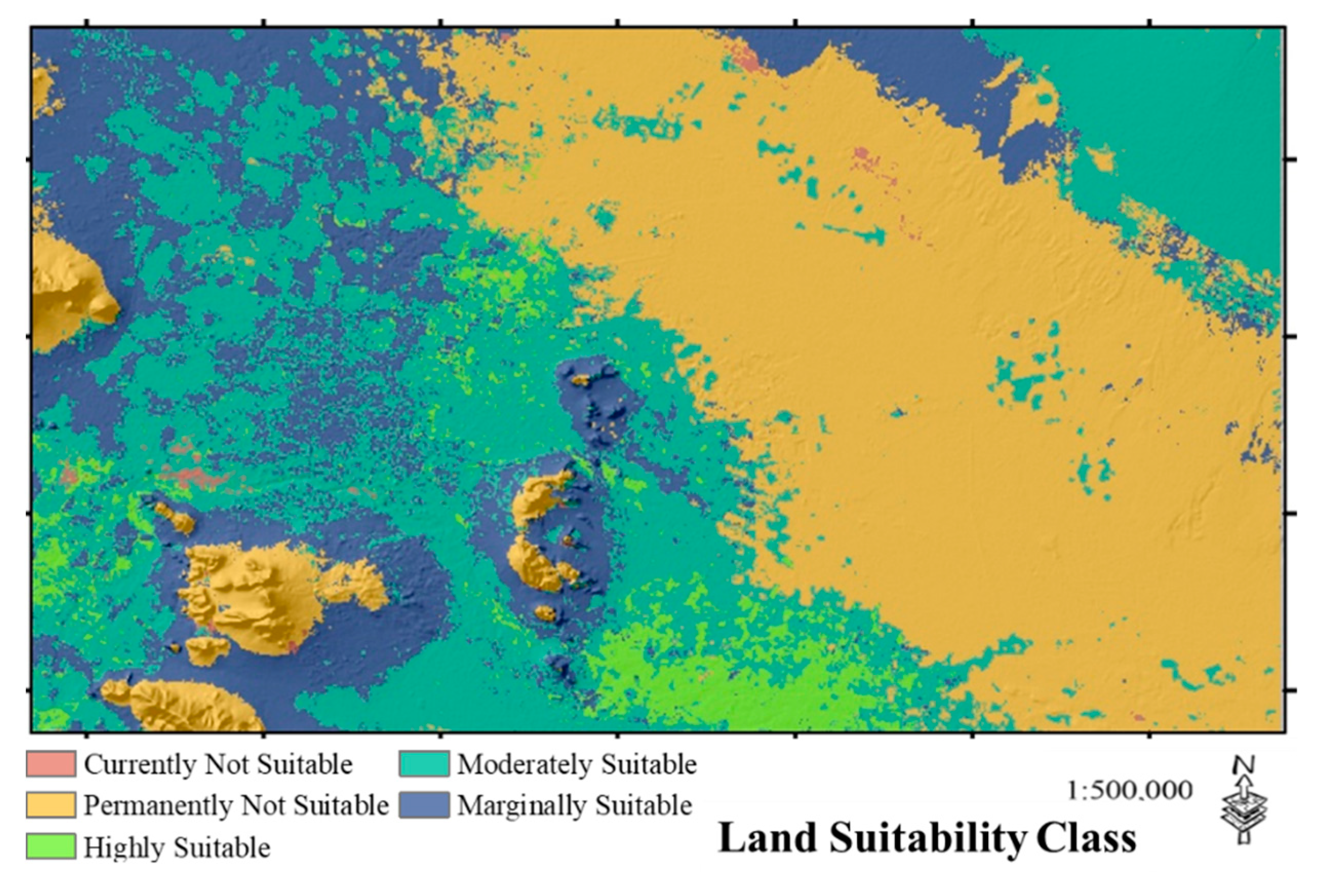
3.4. Land Characteristics, Qualities, Management and Conservation of DSM Soil Taxa Relative to Land Use

Modeling the spatial distribution of soil taxonomic classes using ML algorithms (e.g., ensemble models) based on the SCORPAN approach [9] provides valuable information for better understanding and management of soil resources in the study area. Importantly, for biomass production, mapping at the Great group and Subgroup it gives a greater understanding of land characteristics and qualities relative to proposed land use and required for soil management [27].

Eight out of the nine Subgroups that were predicted by the ensemble model were in Aridisols order (Figure 4k). The soil moisture regime of Aridisols is aridic, a condition in which for more than half of the cumulative days of a normal year, there is no water available for mesophyte plants [27,55]. Therefore, the use of Aridisols is limited by the lack of water, and without irrigation, they are useful only for low productive rangeland, seasonal gazing, and non-agricultural uses [56].

To show the relationships between soil taxonomic classes and soil functions, the spatial distributions of soil suitability classes for wheat production is presented in Figure 6. This map indicates that most of the area (about 43%) is not suitable (N2 suitability class) for wheat production, while only a small portion (4.25%) has the characteristics that are well suited (S1) for wheat. Following unsuitable areas, 32.77% and 20.10% of the study area were classified as moderately (S2) and marginally (S3) suitable, respectively.

Despite the criteria that were used to distinguish soil taxonomic classes are not the same as the ones used in suitability and, moreover in soil taxonomy soil properties that affect their responses to the management and use are often considered in the family level, an overall consistency between the spatial distributions of soil taxonomic classes and soil suitability classes was revealed (Figure 4 and Figure 6).

Areas with Salids (i.e., Typic Haplosalids and Gypsic Haplosalids) corresponded to areas with suitability class of N2 (Figure 4 and Figure 6). Very high content of salts is the most important limitation of Salids, which were predicted at the center of the study area (Figure 4i). Therefore, without major leaching and drainage practices, these soils are not suitable for agricultural uses. Also some areas of Orthents (i.e., Typic Torriorthents) because of high contents of coarse fragments or high slope degree, are placed in N2 suitability class. Most of the Torriorthents in Iran, because of shallow depth, high gravel content or coarse texture, are not suitable for crop production and are generally considered as marginally suitable rangelands [56]. Overall, Aridisols have several limitations which affect their suitability for sustainable agricultural uses [56]. The limitations of areas with N2 suitability class are so severe that at the current condition the sustained successful use of them is impossible.

Most Argids in the study area are moderately suitable (S2) for wheat production. High clay content, moderate salt content and slope degree in the study area are the main limiting factors of Argids, hence they are classified as S2. The argillic horizon in Argids may restrict vertical movement of water through the soils and thus results in poor drainage conditions due to its fine texture [57,58].

Soils in Gypsids suborders located at the north-east of the study area (Figure 4k) are often not suitable for sustainable crop production. Gypsids are mainly associated with S3 land suitability class. Therefore they have limitations which in the aggregate are severe for sustainable application of wheat production. These limitations are so severe that reduce productivity and benefits to such level that expenditure are only marginally justified. Main problems that preclude the sustainable use of Gypsids for wheat can be attributed to high gypsum content, land subsidence (because gypsum is relatively high soluble), coarse texture, and low water holding capacity [57]. Lithic Haplogypsids, in addition to the limitations arising from the high content of gypsum and water scarcity (aridic soil moisture regime), have a lithic contact within 50 cm of the soil surface, which limits water and roots penetration into the soil [27,55].

High calcium carbonate content is the main limiting factor of Calcids for agricultural land uses [57], specifically petrocalcic and petrogypsic horizons; which may occur in Calcids and Gypsids respectively. This is because these are cemented or indurated horizons that can preclude penetration of water and roots in the soils. Moreover, these cemented horizons may impede excavation in non-agricultural uses of land (e.g., building and landscaping). In Iran, calcium carbonate concentration up to 35% in soil does not significantly affect irrigated wheat production and hence, most soils of the study area did not have major limitations in terms of calcium carbonate content and petrocalcic horizon. Therefore, Typic Haplocalcids which cover only limited areas of the study site were classified as S1. This suitability class indicates that Typic Haplocalcids have no significant limitations for sustained use of wheat or only have minor limitations that do not significantly affect productivity, benefits or inputs levels.

Overall, Aridisols and Entisols have several limitations which affect their suitability for sustainable agricultural uses [58]. Therefore, only limited areas of Aridisols and Entisols under specific management and conditions (e.g., major land improvement programs) could be irrigated and used for crop production.

4. Conclusions

Several individual models, including ANN, MnLR, SVM, RF, DT, BN, and SMnLR, were used to predict the spatial distribution of the USDA soil taxonomic classes in Isfahan region (Iran). The overall accuracy (OA) and area under the curve (AUC) decreased from Order, Sub-order, Great group and Subgroup levels for all investigated models. However, among all individual models, RF showed the best performance in terms of OA at the Order (0.87), Sub-order (0.52), Great group (0.46) and Subgroup (0.41) levels. The worst performing model results were achieved using MnLR at the Order (0.64), Sub-order (0.40), Great group (0.34) and Subgroup (0.34) levels.

In terms of the more robust kappa (κ) statistic and AUC value, the results suggest that the best soil taxonomic levels were the Order and Sub-order, because they consistently returned the largest values. In this regard, the RF model was largest for the Order (κ = 0.57, AUC = 0.75) and Sub-order (κ = 0.38, AUC = 0.60) levels. The next best was SMnLR for Order (κ = 0.51, AUC = 0.71) and Sub-order (κ = 0.37, AUC = 0.59). The worst results were achieved using the MnLR for Order (κ = 0.23, AUC = 0.66) and Sub-order (κ = 0.25, 0.46).

Regarding the sensitivity analysis, the ensemble model showed better performance as compared with the individual approaches and decreased the false prediction of soil class taxa at Subgroup level. In addition, the average users’ accuracy or positive predicted values (PPV) of ensemble model increased the correctly predicted classes at Subgroup level in comparison with individual approaches.

With respect to ensemble modeling, a combined model developed by MnLR from the seven data modeling techniques exceeded all the models in performance and to predict soil taxonomic classes at different levels (Ensemble.2). This is because the multinomial ensemble model is able to combine strengths of individual models. The ensemble model positively improved the validation criteria in comparison with the best individual model (RF), except at the Order level. Here the OA was larger than the best performing individual model (i.e., RF) with an improvement between 27–35% at all levels except the Order. This was also the case with respect to the κ statistic with an improvement between 43–60%. Furthermore, AUC values increased 5–22% in comparison with the best performing individual model (i.e., RF). Therefore, the application of the ensemble model was overall quite successful, as it provided a highly accurate prediction for all soil taxonomy levels over and above the individual models.

Soil maps created via the DSM approach, such as demonstrated in this study, showed the soils that are prone to degradation (e.g., Typic Calcigypsids and Typic Haplocalcids) and to need to be carefully managed and conserved to avoid further land degradation. Further, for irrigation purposes, an accurate delineation of soils with high salinity or high salinity risk (e.g., Typic Haplosalids and Gypsic Haplosalids) is crucial to ensure sustainable irrigation schemes.

In particular, the presence of gypsic and calcic horizons (e.g., Gypsids and Calcids) and also the impermeable horizons, such as petrogypsic and petrocalcic, have a strong impact on root developments, plant growth, and crop production under irrigation. Furthermore, saline soil affects crops through inhibiting the uptake of water. Percolating water dissolves gypsum, calcium, and salts and stagnates at the top of the gypsic and calcic horizons, creating a perched water-table, often resulting in an accumulation of gypsum, calcium, and salts. The resulting high water-table may rise to the soil surface, leaving salts, calcium, and gypsum. Under these conditions, the performance of crops will be affected by accumulation of the aforementioned materials.

Future work will assess the uncertainty of prediction of individual and ensemble models and how they can be used to assess specific soil functions. There is also a need to investigate the possibility of incorporating probabilities of prediction in the ensemble.

References

1. Adhikari, K.; Hartemink, A.E. Linking soils to ecosystem services-A global review. Geoderma 2016, 262, 101–111. [Google Scholar] [CrossRef]
2. Dominati, E.; Patterson, M.; Mackay, A. A framework for classifying and quantifying the natural capital and ecosystem services of soils. Ecol. Econ. 2010, 69, 1858–1868. [Google Scholar] [CrossRef]
3. Brungard, C.W.; Boettinger, J.L.; Duniway, M.C.; Wills, S.A.; Edwards, T.C. Machine learning for predicting soil classes in three semi-arid landscapes. Geoderma 2015, 239, 68–83. [Google Scholar] [CrossRef]
4. Jafari, A.; Finke, P.A.; Van de Wauw, J.; Ayoubi, S.; Khademi, H. Spatial prediction of USDA-great soil groups in the arid Zarand region, Iran: Comparing logistic regression approaches to predict diagnostic horizons and soil types. Eur. J. Soil Sci. 2012, 63, 284–298. [Google Scholar] [CrossRef]
5. Pahlavan-Rad, M.R.; Khormali, F.; Toomanian, N.; Brungard, C.W.; Kiani, F.; Komaki, C.B.; Bogaert, P. Legacy soil maps as a covariate in digital soil mapping: A case study from Northern Iran. Geoderma 2016, 279, 141–148. [Google Scholar] [CrossRef]
6. Zeraatpisheh, M.; Ayoubi, S.; Jafari, A.; Finke, P. Comparing the efficiency of digital and conventional soil mapping to predict soil types in a semi-arid region in Iran. Geomorphology 2017, 285, 186–204. [Google Scholar] [CrossRef]
7. Caubet, M.; Dobarco, M.R.; Arrouays, D.; Minasny, B.; Saby, N.P. Merging country, continental and global predictions of soil texture: Lessons from ensemble modelling in France. Geoderma 2019, 337, 99–110. [Google Scholar] [CrossRef]
8. Ma, Y.X.; Minasny, B.; Malone, B.P.; McBratney, A.B. Pedology and digital soil mapping (DSM). Eur. J. Soil Sci. 2019, 70, 216–235. [Google Scholar] [CrossRef]
9. McBratney, A.B.; Santos, M.M.; Minasny, B. On digital soil mapping. Geoderma 2003, 117, 3–52. [Google Scholar] [CrossRef]
10. Heung, B.; Ho, H.C.; Zhang, J.; Knudby, A.; Bulmer, C.E.; Schmidt, M.G. An overview and comparison of machine-learning techniques for classification purposes in digital soil mapping. Geoderma 2016, 265, 62–77. [Google Scholar] [CrossRef]
11. Minasny, B.; McBratney, A.B. Digital soil mapping: A brief history and some lessons. Geoderma 2016, 264, 301–311. [Google Scholar] [CrossRef]
12. Adhikari, K.; Minasny, B.; Greve, M.B.; Greve, M.H. Constructing a soil class map of Denmark based on the FAO legend using digital techniques. Geoderma 2014, 214, 101–113. [Google Scholar] [CrossRef]
13. Kovačević, M.; Bajat, B.; Gajić, B. Soil type classification and estimation of soil properties using support vector machines. Geoderma 2010, 154, 340–347. [Google Scholar] [CrossRef]
14. Behrens, T.; Förster, H.; Scholten, T.; Steinrücken, U.; Spies, E.D.; Goldschmitt, M. Digital soil mapping using artificial neural networks. J. Plant Nutr. Soil Sci. 2005, 168, 21–33. [Google Scholar] [CrossRef]
15. Taghizadeh-Mehrjardi, R.; Nabiollahi, K.; Minasny, B.; Triantafilis, J. Comparing data mining classifiers to predict spatial distribution of USDA-family soil groups in Baneh region, Iran. Geoderma 2015, 253, 67–77. [Google Scholar] [CrossRef]
16. Górecki, T.; Krzyśko, M. Regression methods for combining multiple classifiers. Commun. Stat.-Simul. C. 2015, 44, 739–755. [Google Scholar] [CrossRef]
17. Swiderski, B.; Osowsk, S.; Kruk, M.; Barhoumi, W. Aggregation of classifiers ensemble using local discriminatory power and quantiles. Expert Syst. Appl. 2016, 46, 316–323. [Google Scholar] [CrossRef]
18. Román Dobarco, M.; Arrouays, D.; Lagacherie, P.; Ciampalini, R.; Saby, N.P.A. Prediction of topsoil texture for Region Centre (France) applying model ensemble methods. Geoderma 2017, 298, 67–77. [Google Scholar] [CrossRef]
19. Diks, C.G.H.; Vrugt, J.A. Comparison of point forecast accuracy of model averaging methods in hydrologic applications. Stoch. Environ. Res. Risk Assess. 2010, 24, 809–820. [Google Scholar] [CrossRef] [Green Version]
20. Wasson, T.; Hartemink, A.J. An ensemble model of competitive multi-factor binding of the genome. Genome Res. 2009, 19, 2101–2112. [Google Scholar] [CrossRef] [Green Version]
21. Malone, B.P.; Minasny, B.; Odgers, N.P.; McBratney, A.B. Using model averaging to combine soil property rasters from legacy soil maps and from point data. Geoderma 2014, 232, 34–44. [Google Scholar] [CrossRef]
22. Padarian, J.; Minasny, B.; McBratney, A.B.; Dalgliesh, N. Predicting and mapping the soil available water capacity of Australian wheatbelt. Geoderma Reg. 2014, 2, 110–118. [Google Scholar] [CrossRef]
23. Hartemink, A.E. The use of soil classification in journal papers between 1975 and 2014. Geoderma Reg. 2015, 5, 127–139. [Google Scholar] [CrossRef]
24. Taghizadeh-Mehrjardi, R.; Sarmadian, F.; Minasny, B.; Triantafilis, J.; Omid, M. Digital mapping of soil classes using decision tree and auxiliary data in the Ardakan region, Iran. Arid Land Res. Manag. 2014, 28, 147–168. [Google Scholar] [CrossRef]
25. Jaafarian, M.A. Past history and evolutionary steps of Zayandeh-rud Valley. Res. J. Isfahan Univ. 1986, 1, 15–31. (In Persian) [Google Scholar]
26. Toomanian, N.; Jalalian, A.; Khademi, H.; Eghbal, M.K.; Papritz, A. Pedodiversity and pedogenesis in Zayandeh-rud Valley, central Iran. Geomorphology 2006, 81, 376–393. [Google Scholar] [CrossRef]
27. Soil Survey Staff. Keys to Soil Taxonomy, 10th ed.; United States Department of Agriculture: Washington, DC, USA, 2006.
28. Conrad, O.; Bechtel, B.; Bock, M.; Dietrich, H.; Fischer, E.; Gerlitz, L. System for Automated Geoscientific Analyses (SAGA) v. 2.1.4. Geosci. Model Dev. 2015, 8, 1991–2007. [Google Scholar] [CrossRef] [Green Version]
29. National Cartographic Center; Research Institute of NCC: Tehran, Iran, 2010; Available online: www.ncc.org.ir (accessed on 21 August 2010).
30. European Space Agency. GMES Sentinel-2 mission requirements document. In Technical Report Issue 2 Revision 1; European Space Agency: Paris, France, 2010. [Google Scholar]
31. Wulder, M.A.; White, J.C.; Loveland, T.R.; Woodcock, C.E.; Belward, A.S.; Cohen, W.B.; Fosnight, E.A.; Shaw, J.; Masek, J.G.; Roy, D.P. The global Landsat archive: Status, consolidation, and direction. Remote Sens. Environ. 2016, 185, 271–283. [Google Scholar] [CrossRef] [Green Version]
32. Mulder, V.L.; De Bruin, S.; Schaepman, M.E.; Mayr, T.R. The use of remote sensing in soil and terrain mapping—A review. Geoderma 2011, 162, 1–19. [Google Scholar] [CrossRef]
33. Andronikov, V.; Dobrolvshiy, G. Theory and methods for the use of remote sensing in the study of soils. Mapp. Sci. Remote Sens. 1991, 28, 92–101. [Google Scholar]
34. Moameni, A.; Zink, J.A. Application of statistical quality control charts and geostatistics to soil quality assessment in a semi-arid environment of south-central Iran. ITC J. 1997, 3, 1–26. [Google Scholar]
35. Alpaydin, E. Introduction to Machine Learning; MIT Press: Cambridge, MA, USA, 2010. [Google Scholar]
36. Marquardt, D.W. An algorithm for least-squares estimation of nonlinear parameters. J. Soc. Ind. Appl. Math. 1963, 11, 431–441. [Google Scholar] [CrossRef]
37. Vapnik, V. The Nature of Statistical Learning Theory; Springer: New York, NY, USA, 1995. [Google Scholar]
38. Ivanciuc, O. Applications of support vector machines in chemistry. Rev. Comp. Ch. 2007, 23, 291. [Google Scholar]
39. Hsu, S.-H.; Hsieh, J.P.A.; Chih, T.C.; Hsu, K.C. A two-stage architecture for stock price forecasting by integrating self-organizing map and support vector regression. Expert Syst. Appl. 2009, 36, 7947–7951. [Google Scholar] [CrossRef] [Green Version]
40. Murthy, S.K. Automatic construction of decision trees from data: A multi-disciplinary survey. Data Min. Knowl. Discov. 1998, 2, 345–389. [Google Scholar] [CrossRef]
41. Breiman, L. Random forests. Mach. Learn. 2001, 45, 5–32. [Google Scholar] [CrossRef]
42. Amit, Y.; Geman, D. Shape quantization and recognition with randomized trees. Neural Comput. 1997, 9, 1545–1588. [Google Scholar] [CrossRef]
43. Rudiyanto, M.B.; Setiawan, B.I.; Saptomo, S.K.; McBratney, A.B. Open digital mapping as a cost-effective method for mapping peat thickness and assessing the carbon stock of tropical peatlands. Geoderma 2018, 313, 25–40. [Google Scholar] [CrossRef]
44. Hartemink, A.J. Bayesian networks and informative priors: Transcriptional regulatory network models. In Bayesian Inference for Gene Expression and Proteomics; Do, K., Müller, P., Vannucci, M., Eds.; Cambridge University Press: Cambridge, UK, 2006; pp. 401–424. [Google Scholar]
45. Robinson, J.W.; Hartemink, A.J. Learning non-stationary dynamic Bayesian networks. J. Mach. Learn. Res. 2010, 11, 3647–3680. [Google Scholar]
46. Taalab, K.; Corstanje, R.; Zawadzka, J.; Mayr, T.; Whelan, M.J.; Hannam, J.A.; Creamer, R. On the application of Bayesian networks in digital soil mapping. Geoderma 2015, 259, 134–148. [Google Scholar] [CrossRef]
47. Dlamini, W.M. Application of Bayesian networks for fire risk mapping using GIS and remote sensing data. GeoJournal 2011, 76, 283–296. [Google Scholar] [CrossRef]
48. Krishnapuram, B.; Carin, L.; Figueiredo, M.A.T.; Hartemink, A.J. Sparse multinomial logistic regression: Fast algorithms and generalization bounds. IEEE Trans. Pattern Anal. Mach. Intell. 2005, 27, 957–968. [Google Scholar] [CrossRef] [PubMed]
49. Narlikar, L.; Hartemink, A. Sequence features of DNA binding sites reveal structural class of associated transcription factor. Bioinformatics 2006, 22, 157–163. [Google Scholar] [CrossRef] [PubMed]
50. Heuvelink, G.B.M.; Bierkens, M.F.P. Combining soil maps with interpolations from point observations to predict quantitative soil properties. Geoderma 1992, 55, 1–15. [Google Scholar] [CrossRef]
51. Granger, C.W.J.; Ramanathan, R. Improved methods of combining forecasts. J. Forecast. 1984, 3, 197–204. [Google Scholar] [CrossRef]
52. Giasson, E.; Figueiredo, S.; Tornquist, C.; Clarke, R. Digital soil mapping using logistic regression on terrain parameters for several ecological regions in Southern Brazil. In Digital Soil Mapping with Limited Data; Hartemink, A.E., McBratney, A.B., Mendonça-Santos, M.L., Ahrens, R.L., Eds.; Springer: Cham, Switzerland, 2008; pp. 225–232. [Google Scholar]
53. Stum, A.K.; Boettinger, J.L.; White, M.A.; Ramsey, R.D. Random Forests Applied as a Soil Spatial Predictive Model in Arid Utah. In Digital Soil Mapping: Bridging Research, Environmental Application, and Operation; Boettinger, J.L., Howell, D.W., Moore, A.C., Hartemink, A.E., Kienast-Brown, S., Eds.; Springer: Dordrecht, The Netherlands, 2010; pp. 179–190. [Google Scholar] [Green Version]
54. Hosmer, D.W.; Lemeshow, S.; Sturdivant, R.X. Applied Logistic Regression; John Wiley & Sons: Hoboken, NJ, USA, 2013. [Google Scholar]
55. Buol, S.W.; Southard, R.J.; Graham, R.C.; Mcdaniel, P.A. Soil Genesis and Classification; John Wiley & Sons, Inc.: Hoboken, NJ, USA, 2011. [Google Scholar]
56. Roozitalab, M.H.; Toomanian, N.; Ghasemi Dehkordi, V.R.; Khormali, F. Major soils, properties, and classification. In The Soils of Iran; Roozitalab, M.H., Siadat, H., Farshad, A., Eds.; Springer: Berlin/Heidelberg, Germany, 2018; pp. 93–147. [Google Scholar]
57. Khademi, H.; Mermut, A.R. Micromorphology and classification of Argids and associated gypsiferous Aridisols from central Iran. Catena 2003, 54, 439–455. [Google Scholar] [CrossRef]
58. Gharaee, H.A.; Mahjoory, R.A. Characteristics and geomorphic relationships of some representative Aridisols in southern Iran. Soil Sci. Soc. Am. J. 1984, 48, 115–119. [Google Scholar] [CrossRef]
Figure 1. Location of study area in Iran (a); soil samples distribution (b); a digital elevation model (c) and geomorphology map of the region (d). Codes of geomorphology map refer to Supplementary Materials.
Soilsystems 03 00037 g001
Figure 2. The overall accuracy (a), kappa index (b) and area under the curve (AUC) (c) of all models for different levels of soil taxonomic.
Soilsystems 03 00037 g002
Figure 3. The importance of variables used for predicting soil classes in four taxonomic levels: Order (a), Sub-order (b), Great group (c) and Subgroup (d). Codes refer to Table 2.
Soilsystems 03 00037 g003
Figure 4. The spatial distribution of soil classes at Subgroup level using different spatial models: Multinomial Logistic Regression (a); Artificial Neural Networks (b); Support Vector Machines (c); Decision Tree (d); Random Forest (e); Bayesian Networks (f); Sparse Multinomial Logistic Regression (g); Ensemble.1 (h) and Ensemble.2 (i).
Soilsystems 03 00037 g004
Figure 5. The spatial distribution of soil classes at Subgroup level in a smaller area using different spatial models: Random Forest (a) and Ensemble.2 (b). GHS: Gypsic Haplosalids; Lithic Haplogypsids: LHG; Typic Calciargids: TCA; Typic Calcigypsids: TCG; Typic Haploargids: THA; Typic Haplocalcids: THC; Typic Haplogypsids: THG; Typic Haplosalids: THS; Typic Torriorthents: TTO.
Soilsystems 03 00037 g005
Figure 6. Spatial distribution of land suitability classes for irrigated wheat.
Soilsystems 03 00037 g006