Coupled Biological and Abiotic Mechanisms Driving Carbonyl Sulfide Production in Soils

Abstract

Understanding soil production of the trace gas carbonyl sulfide (OCS) is key to its use as a tracer of ecosystem function. Underlying its application is the observation that vascular plants consume atmospheric OCS via their stomatal pores in proportion with CO₂ photosynthesis and that soil fluxes of OCS are negligible in comparison. Recent soil-centered studies demonstrate that soils can produce OCS and contribute as much as a quarter of the atmospheric terrestrial flux. Despite the potential widespread importance of soil OCS emissions, insufficient data exist to predict variations in OCS production across ecosystems, and the chemical and biological drivers of OCS production are virtually unknown. In this study, we address this knowledge gap by investigating variables controlling OCS soil production including soil physical and chemical properties, microbial community composition, and sulfur speciation in two independent surveys. We found that soil OCS production was nearly ubiquitous across the 58 sites, increased exponentially with temperature, and was insensitive to visible light conditioning. Soil pH, N, and C/N were predictors of OCS soil production rates in both soil surveys. Patterns in soil S speciation and predicted microbial S-cycling pathways both pointed to S-containing amino acids such as cysteine and methionine and their derivatives as potential precursors for OCS production. Elevated sulfate levels were associated with OCS production in some soils. This study provides new mechanistic insight into OCS production in soils and presents strategies to represent soil OCS fluxes that facilitate the use of OCS as a tracer for leaf-level processes related to carbon and water cycling.

1. Introduction

Soils may be either a source or sink of OCS, or both, and the conditions that dictate this balance are not well resolved. Maximum soil uptake of OCS is generally observed at intermediate moisture levels that support both gas diffusion and microbial activity, notably OCS hydrolysis by carbonic anhydrase (CA) [1]. Until recently, emissions of OCS by soils were thought to be a feature only of wetland systems (reviewed in [2]), but periods of net soil OCS emission have now been reported in forest, grassland, and cropland ecosystems [3,4,5,6,7]. Soil incubation studies have further shown that both OCS production and consumption are widespread in soils, and the balance of these two gross fluxes drives the net soil–atmosphere OCS exchange [8,9,10]. OCS production has also been observed from plant components (e.g., roots, non-photosynthetic plant tissues) [7,11] and non-vascular plants (e.g., liverwort, moss) [12,13]. The mechanism for OCS production and its sensitivity to environmental conditions are poorly understood, which limits efforts to account for OCS soil fluxes and represents a gap in our understanding of biosphere–atmosphere sulfur cycling. Process-level representation of soil OCS cycling is needed to reduce uncertainty in the global OCS budget. In addition, constraining spatial and temporal variability in soil-atmosphere OCS exchange will improve estimates of large-scale, leaf-level processes (e.g., stomatal conductance and photosynthetic CO₂ uptake) derived from the application of OCS as an atmospheric tracer [14].

OCS production in soils could be driven by biological and/or abiotic processes, and divergent mechanisms have been proposed. Abiotic thermo- and photo-degradation reactions involving still unknown chemical and biological components or pathways may be a driver of OCS production [8,11,13,15]. Soil OCS production rates depend exponentially on temperature [7,8,10], increase with light [5,11], and persist at similar rates when the same soil sample is moist and dry [10]. Furthermore, OCS production persists in soils following biological inactivation by autoclaving [11,16]. These observations suggest an abiotic mechanism for OCS production such as photo-thermal degradation of sulfur compounds, which may be indirectly coupled to biological production of precursor compounds by soil microbes and plants. Additionally, some bacterial and fungal isolates emit OCS, though observations of OCS consumption are more frequent [17,18]. Known microbial metabolisms directly producing OCS include metabolism of carbon disulfide (CS₂) [19], thiocyanate (SCN⁻) [20,21,22,23,24,25], and isothiocyanate [26]. While enzymes associated with these production pathways have been described in some organisms (e.g., thiocyanate hydrolase [24]), their contributions to OCS soil fluxes have not been evaluated. New efforts are needed to identify the dominant mechanism(s) driving OCS production in soils.

Microbes participate in a wide array of S transformations in soil that may include the production of OCS precursors. Most sulfur in soils is contained in soil organic matter (>95% of total S) including microbial biomass (~1% S) [27,28]. Microbes mineralize organic S compounds to inorganic sulfate (SO₄²⁻), the bioavailable form for plant assimilation and for microbial assimilatory needs. Conversely, microbes carry out dissimilatory S redox reactions. For example, sulfate reducing bacteria and sulfur oxidizing bacteria gain energy through interconversions between sulfate (SO₄²⁻) and sulfide (H₂S), and their intermediates. As a result of these assimilatory and dissimilatory processes, soil systems contain a diverse spectrum of S compounds that may serve as OCS precursors. A number of potential OCS precursors have been evaluated through soil amendments with mixed results. For example, cystine, cysteine, and thiocyanate amendments were found to stimulate OCS production in one study [29], while OCS production was only observed in response to thiocyanate addition but not to cysteine, methionine, sulfate, or elemental S in a second study [30]. Plants have been shown to release OCS as a result of the degradation of unstable S-containing intermediates such as aromatic isothiocyanates [31] and thiocarbamates [32]. The most extensive work on precursors to OCS production has been performed in aquatic systems, where OCS production has been observed from filtered natural water amended with disulfides (e.g., cystine), sulfides (e.g., methionine), thiols (e.g., cysteine), and thiocyanates (e.g., isothiocyanate) (

Table 1. Previously reported OCS production from S species from aquatic systems (filtered natural water).

Compound	Classification	Non-Photochemical Production	Photo-Chemical Production (UV)	References
Cysteine (CYS)	Thiol, R-SH	N	Y	[33,34,36,37,40]
Methionine (MET)	Thioether (organic sulfide) R-S-R’	N	uncertain	[33,34,37]
Glutathione (GSH)	Thiol, R-SH	Y	Y	[33,34]
3-Mercaptopropionic acid (3-MPA)	Thiol, R-SH	N	Y	[34]
Methyl mercaptan (MeSH)	Thiol, R-SH	N	Y	[34]
Sulfide	Sulfide, HS−	-	Y	[34]
Dimeric disulfide (Na-GSSG)	Organic disulfide, R-S-S-R’	N	N	[34]
Methanesulfonic acid (MSA)	Sulfonate, R-O-SO2	N	N	[34]

) [33,34,35,36]. OCS production from aquatic systems has been found to depend on light (particularly UV light), oxygen levels, and the presence of dissolved organic matter, and proposed chemical mechanisms include photochemical degradation of S compounds [33,36,37,38] and light-independent reactions of sulfur radicals (thiyls) with carbonyl compounds [34,39]. A main challenge is to determine whether OCS production in different soils are related to one or more common microbial S-cycling pathway(s) and related S compound(s).

In this study, we investigate the role of physical, chemical, and microbial processes as drivers of OCS production in soils. Our aim was to determine whether common abiotic, biotic, or coupled abiotic–biotic processes dominate OCS production rates in different soils. Our approach was to collect soils from various locations, biomes, and land use types in two independent soil surveys that were conducted predominantly in the United States (Survey 1; 20 sites) and Europe (Survey 2; 38 sites). Net OCS fluxes were measured on air-dried soils, which reflect predominantly abiotic OCS production processes given that microbe-mediated OCS consumption ceases under moisture limitation [10]. To elucidate potential mechanisms, we measured the temperature (Survey 1) and light (Survey 2) sensitivity of OCS production in soils. Recognizing that many chemical, physical, and microbial factors operate and are coupled within the soil system, we characterized 75 properties in Survey 1 including S and sulfate concentrations, S speciation by X-ray absorption near edge structure (XANES) spectroscopy, and microbial community composition and 12 widely measured properties in Survey 2 that are useful for predictive models including soil C, N, pH, and redox. In this paper, we analyze this extensive data set to address the following hypotheses: (1) the dominant production mechanism for OCS in soils is abiotic photo-thermal degradation of S compounds; (2) direct microbial OCS production pathways do not significantly contribute to OCS fluxes in soils; and (3) microbial and plant S cycling indirectly drive OCS production in soils through production of S intermediates. Our results will provide new mechanistic insight and predictive power for describing the production of OCS in soils.

2. Materials and Methods

In this study, two separate surveys were conducted on soils of different origins, using similar methods that resulted in independent, yet complementary data sets. Survey 1 soils were part of an experiment designed to investigate the role of temperature in regulating OCS flux, while Survey 2 soils were used for experiments exploring the response of OCS to light. Differences and similarities between the survey methods are summarized in

Table 2. Side-by-side comparison of soil collection, processing, and analysis methods for Surveys 1 and 2.

Soil Collection	Survey 1	Survey 2
Sites	20	38
Region	United States, Cambodia	Europe
Biomes	Arid, Mediterranean, Boreal, Temperate, Tropical	Arid, Mediterranean, Boreal, Temperate
Land use	Cropland, Desert, Grassland, Deciduous Forest, Evergreen Forest, Peatland	Cropland, Orchard, Grassland, Deciduous Forest, Evergreen Forest, Peatland
Sampling depth	0 to 10 cm (after removing litter)	0 to 10 cm (after removing litter)
Samples	3 within a 1-m sampling radius	3–5 within 5-m radius
Soil Processing	Survey 1	Survey 2
Sampling depth	Replicates kept separate	Replicates homogenized
Sieve mesh size	2 mm (Humboldt Mfg., Elgin, IL, USA)	5 mm
Pre-treatment	Air-dried 3 days, wet to 30% WHC, incubated 7 days at 22.5 °C in the dark	Soils at field moisture untreated
Final treatment	Air-dried for a median of 45 days	Air-dried for 7–14 days
Flux Measurements	Survey 1	Survey 2
Soil amount	80 g dry soil	350–400 g dry soil
Measurement chamber	1-L PFA chambers (100-1000-01, Savillex, Eden Prairie, MN, USA). Surface area of 0.0078 m2	0.825 L glass jars with customized glass lid with stainless steel and PTFE ports. Surface area of 0.0062 m2
Acclimation	24 h dark at 22.5 °C	2–3 days under 12 h dark/12 h light photoperiod at 17 °C
Treatments	Temperature ramp (11.5 °C to 37.5 °C; dark only)	Light conditioning and temperature artifact (dark at 17 °C; light at 23 °C)
Inlet air source	Room air passed through buffer volume (2 L PFA chamber)	Scrubbed ambient air with CO2 and OCS added to approximately 420 ppm CO2 and 500 ppt OCS.
Flow rate	0.3 L min−1	0.25 L min−1
Temperature control	Water bath [8]	Customized climate-control chamber (MD1400, Snijders, Tillburg, The Netherlands)
Dynamic flow sequence	Inlet (10 min), N2 tank background (10 min), and outlet (40 min)	Each component 2 min
Time averaged	Last 4 min inlet, 4 min for N2, and 8 min for outlet measurements.	Last 20 s for all measurements.
Soil Characterization	Survey 1	Survey 2
Measured properties (pre-treatment)	WHC, microbial biomass, microbial community composition (DNA), metatranscriptomes (RNA)	WHC, soil moisture
Measured properties (final treatment)	OCS and CO2 fluxes, BD, C, N, pH, texture, soil moisture, S, other elements, SO4, XANES	OCS and CO2 fluxes, BD, C, N, pH, texture, redox potential
pH method	1:2.5 soil-water ratio	1:5 soil-water ratio
Texture method	Multi-wavelength laser diffraction particle analyzer (LS 13 320 MW, Beckman Coulter, Brea, CA, USA)	Sedimentation method (INRA method SOL-0302).
C and N method	Elemental analyzer (NA-1500, Carlo-Erba, Milan, Italy)	Gas chromatography and catharometer (corrected for CaCO3; INRA methods NF-ISO-13878, NF-ISO-10694)
Microbial biomass method	Chloroform fumigation-potassium sulfate extraction method [43]	Chloroform fumigation-potassium sulfate extraction method [44,45].

and additional detail regarding the Survey 1 and 2 methods are described in [8,41] and [10,15], respectively.

2.1. Soil Collection and Processing

Soil samples were collected from the uppermost 10 cm (litter excluded) at 20 sites in Survey 1 and 38 sites in Survey 2 (Table 2) covering a range of biomes and land use types (Table 2 and Table S1). Soils were sieved and used to determine field moisture and soil water holding capacity (WHC). Following sieving, soils were pre-treated in Survey 1 (Table 2) by transferring 80 g DW (soil dry weight) to sterilized half-pint mason jars, adjusting soil moisture levels with sterile nanopure water to 30% WHC, and incubating aerobically at 22.5 °C for seven days in the dark. This pre-treatment was done for comparability to identical soil preparations in a separate, simultaneous study on the microbial drivers of OCS consumption in moist soils [41]. At 30% WHC, soils are sufficiently moist to support microbial activity, but not so wet as to impede gas diffusion through the soil matrix [42]. The final treatment for both surveys involved transferring soils from either the 30% WHC incubation pre-treatment (Survey 1) or the untreated field-moist soils (Survey 2) to aluminum trays to dry by evaporation. After air drying, soils were transferred to the gas flux measurement chambers to briefly acclimatize (Table 2), after which OCS and CO₂ gas fluxes were measured on the dry soils.

2.2. Trace Gas Flux Measurements

2.2.1. Trace Gas Flux Procedures and Calculations (Surveys 1 and 2)

Measurement chambers containing air-dried soils were installed on dynamic flow-through systems for OCS exchange measurements. Soil-air gas exchange was determined from differences in OCS and CO₂ mole fractions measured in chamber outlet and inlet air flowing using quantum cascade laser spectrometers at 1 Hz (QCLS, Aerodyne Research, Inc., Billerica, MA, USA for both surveys). The QCLS instrument precision is approximately 2 ppt for OCS at 60 s averaging with an absolute calibration accuracy of 5% for OCS (Aerodyne Research, Inc., Billerica, MA, USA). The measurement setups have been previously described in detail for Survey 1 [8] and Survey 2 [15]. Two modifications were made for Survey 1. Firstly, we modified the experimental setup of [8] to include a buffer volume (2 L PFA chamber) on the gas inlet line to dampen fluctuations in OCS mole fractions in inlet air from the laboratory. Secondly, we corrected OCS mole fraction measurements for water vapor dilution and spectral interferences [8,46] using instrument-specific water vapor dependencies to adjust mole fractions to a common humidity level of 0.010 mol mol⁻¹. The dependencies to water vapor mixing ratio [H₂O] (mol mol⁻¹) was [OCS] (ppb) = −1.05[H₂O] + 0.539. Water vapor corrections were 3% (5%) in the median (95th percentile).

Differences between mole fractions in the flow-through chamber inlet gas and outlet gas were measured along with zero tanks (N₂ tank) or calibration gases according to the dynamic flow sequenced used for each survey (Table 2). Instrument drift was corrected for using N₂ background measurements. For both surveys, fluxes of OCS were determined from the difference between mole fractions at the outlet (c_o) and inlet (c_i) measured, respectively, by the chamber and bypass flow. For example:

$$F=\frac{u}{S}\left(c_o-c_i\right)$$

(1)

where u (mol s⁻¹) is the flow rate of air through the chamber, S is the soil surface area and c_o and c_i are the OCS mixing ratios inside the chamber and the bypass air, respectively. OCS production rates are not significantly different in dry and moist soils, and thus, OCS production rates can be determined from the net fluxes of OCS in air-dried soils in which biological OCS uptake is limited [10]. CO₂ fluxes (F_CO2) were simultaneously determined using Equation (1) in both surveys.

2.2.2. Temperature Response Experiment (Survey 1)

Survey 1 fluxes were for each dry soil replicate over a 5 °C- or 10 °C-step temperature ramp between 10 °C and 40 °C at each temperature for three cycles of the aforementioned 60-min program (inlet, zero, outlet). Soil chambers were placed in a water bath for temperature control. OCS fluxes in the dry soils derived using Equation (1) are reported at 20 °C and 40 °C as F₂₀ and F₄₀, respectively. We fit measurements of the temperature-dependent emission of OCS from dry soils using a least-square fit to the exponential model.

$$F_{abiotic}=\alpha \exp \left(\beta T_{soil}\right)$$

(2)

where $T_{soil}$ is the soil temperature in °C, α and β represent the OCS flux at 0 °C and the temperature sensitivity of OCS emissions, respectively [7,8]. For consistency with previous work, results were reported in the commonly-used Q₁₀ framework [10,47],

$$F_{abiotic}=P_{ref}{Q_{10}}^{\left(T_{soil}-T_{ref}\right)/10}$$

(3)

where $T_{ref}$ is a reference temperature, here taken to be 20 °C, and $P_{ref}$ represents the OCS flux at $T_{ref}$, and the temperature sensitivity terms are analytically related using the following expression: $Q_{10}=\exp \left(\beta \times 10\right)$. We accounted for differences between set (10, 15, 20, 25, 30, 35, and 40 °C) and actual (11.5, 15.5, 20.5, 24.5, 28.5, 33.5, and 37.5 °C) soil temperature during the incubation. The mixing ratios inside the chamber were also converted into volumetric concentration using air temperature measurements in the chamber and assuming an atmospheric pressure of 101.325 kPa. OCS fluxes in desert samples were negative (indicating net uptake even when dry), but became less negative with temperature, indicating either less uptake or more production with increasing temperature (Figure S1), and we applied a zero offset before fitting with an exponential temperature response curve to determine temperature sensitivity parameters (offsets for UT-CR and UT-MO were 1.8 pmol kg⁻¹ min⁻¹ and 0.6 pmol kg⁻¹ min⁻¹, respectively). We adjusted Survey 1 fluxes from 20.5 °C to 17 °C using the observed temperature sensitivity for each soil (Equation (2)) to match the conditions of Survey 2 dark fluxes for plotting purposes only (negative fluxes were not adjusted). All other analyses of F₂₀ are performed on unadjusted flux measurements at 20.5 °C for Survey 1 and 17 °C for Survey 2.

2.2.3. Light Response Experiment (Survey 2)

Soil OCS production rates (F₂₀) were measured in the dark and under visible light (400–700 nm; 500 mol(photons) m⁻² s⁻¹) on dry soils. The dark treatment soil microcosms were covered with aluminum foil and were thermally-regulated at 17 °C. Those that received light were slightly warmer, typically around 23 °C because the light treatment caused a heating artifact [13,15]. This temperature difference was measured during the incubations with stainless temperature probe (three-wire PT100) that measured the temperature of the soil surface at 2–4 cm depth. Q₁₀ was not determined in Survey 2 under light or dark conditions, therefore we did not attempt adjust F₂₀ values (light or dark) to a common temperature for a comparison of light conditioning effects under constant temperature conditions.

2.3. Soil Characterization

2.3.1. Soil Physical, Chemical, and Microbial Community Characterization (Surveys 1 and 2)

Soil characterization performed in both surveys included soil moisture, WHC, bulk density (BD), texture, pH, C, and N following methods detailed in Table 2. Additional information on Survey 1 and Survey 2 methods can be found in [8,41] and [10,15], respectively. Gravimetric (g H₂O g⁻¹ soil) water holding capacity (WHC) was determined from the mass difference before and after 48 h of 105 °C drying of soils saturated (20 g soil in 40 mL nanopure water) for 2 h in stoppered filter funnels (Whatman no. 42, GE Healthcare, Little Chalfont, UK) and then drained for 6 h [48]. Bulk density (BD) was determined from soil mass (10 g) and volume (measured in 15 mL conical tubes). We report soil moisture as the gravimetric (GWC; m/m) or volumetric water content (VWC; v/v) from the mass difference before and after 48 h of 105 °C drying (volume conversion with BD). Soil texture is reported in as the particle distribution of clay (<2 μm), silt (2 μm to 50 μm), and sand (>50 μm) was determined by laser diffraction (Survey 1) and sedimentation (Survey 2) methods, and are reported here on the sedimentation scale for comparability [49]. Soil pH, C, and N were analyzed on dry soils in both surveys. Survey 2 soils were analyzed for redox potential using the same slurry as for pH. Climatic data were derived from 30-year averages (1984-2014) of Climate Research Unit (CRU TS v3.25) data [50].

2.3.2. Soil S Speciation (Survey 1)

We characterized soil S speciation in Survey 1 soils. Directly after the dynamic flux measurement, dry soils were destructively sampled to determine total sulfur, sulfate, and XANES analyses. Elements, including S, were measured by X-ray diffraction spectrometry (Xepos HE XRF Spectrometer, Spectro Analytical Instruments GmbH, Kleve, Germany). Sulfate was measured by ion chromatography (IC) in wet and dry soils (DX-500, Dionex, Thermo Scientific, Waltham, MA, USA) following potassium phosphate (0.016 M KH₂PO₄) or deionized water extractions (1:5 soil to solution, 2 h shaking, centrifuged, filtered 0.2 µm) for total and soluble inorganic sulfate, respectively, thus revealing adsorbed sulfate by difference.

S K-edge XANES spectroscopy identifies the oxidation state and co-ordination environment of soil sulfur by comparison against spectral libraries of known reference compounds [51]. We performed sulfur K-edge XANES (X-ray absorption near-edge structure) spectroscopy on a few milligrams of dry soil under He-atmosphere at beamline 4-3, Stanford Synchrotron Radiation Lightsource (SSRL), using a Si(111) monochromator (energy calibrated by setting the first edge of the in-line thiosulfate standard to 2472.02 eV) and SiLi Vortex detector. Normalized sample spectra were fit with linear combination fitting using Athena software (Demeter 0.9.25, using Ifeffit 1.2.12) [52] and model spectra from the sulfur XANES spectra database (http://www.esrf.eu/home/UsersAndScience/Experiments/XNP/ID21/php.html) provided by the ID21 beamline at the European Synchrotron Radiation Facility. Species with <2% contribution to the fits were disregarded.

2.3.3. Soil Microbial Characterization (Survey 1)

Microbial biomass, community composition, and metatranscriptomes were analyzed in Survey 1 soils. Soil samples were taken at the end of the ‘moist’ pre-treatment (Table 2) and were preserved for DNA- (flash-frozen in liquid nitrogen) and RNA- (LifeGuard^® Soil Preservation Solution, MO BIO Laboratories, San Diego, CA, USA) based analyses. Soil DNA was later extracted from 0.25 g of each replicate (PowerSoil^® DNA Isolation Kit, MO BIO Laboratories, San Diego, CA, USA) and RNA was extracted (PowerSoil^® RNA Isolation Kit, MO BIO) from 1.0 g of one replicate of ten sites (

Table A1. Soil metatranscriptome size and thiocyanate hydrolase (scnC) recovery statistics using BLAST and Pfam function search for assembled CA and assembled CA weighted per million total genes in genome.

Site Name	JGI Project ID	Genome Size (bp)	Assembled scnC		Assembled scnC Million Genes−1
			BLAST	Pfam	BLAST	Pfam
CA-CC	1106757	681,529,179	44	64	40	28
WI-WC	1106758	671,257,491	4	82	52	3
OK-GP	1106759	587,647,789	21	104	73	15
CA-SR2	1106756	521,748,598	91	82	64	71
CA-BB	1106760	303,323,377	33	38	51	44
CA-JRSN	1106761	245,908,234	1	40	65	2 1
HI-KP	1106762	244,931,251	10	49	81	17
CM-DF	1106763	146,941,622	11	12	33	30
CA-SR1	1106764	88,712,635	5	16	72 1	22 1
IL-BV	1106755	65,589,854	43	1	6 1	273 1

¹ Genomes < 0.1 Gbp or with few recovered genes subject to spurious ratios.

). Phylogenetic amplicon iTag DNA sequencing from DNA extract with 16S rRNA (V4) and fungal ITS2 (ITS9F/ITS4R) primers and metatranscriptome sequencing from soil RNA were performed by the Department of Energy Joint Genome Institute (JGI), Walnut Creek, CA, USA. Data sets are available in the JGI Genome Portal (https://genome.jgi.doe.gov/) under JGI proposal ID 2033. Sequence data were collected from the moist-soil pre-treatments, and the patterns in microbial community composition and biomass (and certainly gene expression) may have shifted over the ca. 45-day air dry treatment in uncharacterized ways.

Soils were sampled following the Survey 1 pretreatment for microbial biomass, which was determined by chloroform fumigation of 3 g DW for three days in the dark following [43,44,45]. Specifically, fumigated and non-fumigated soils were extracted with 10 mL 0.5 K₂SO₄ through pre-leached (using 0.5 M K₂SO₄) filter paper (Whatman no. 1, GE Healthcare, Little Chalfont, UK) after one hour of vigorous shaking. Extracts were frozen until dilution (1:3 into DI water) and analysis made on a total organic carbon analyzer (TOC-L, Shimadzu, Tokyo, Japan). The chloroform-labile pool of C or N (EC and EN; ug C or ug N g DW⁻¹) was estimated from the difference between the extracted C or N in fumigated and control samples and converted to microbial biomass (C or N) using microbial C = EC/k_EC or microbial N = EN/k_EN, where k_EC and k_EN represent the microbial C and N mineralization efficiency, taken here to be the constants 0.45 and 0.54, respectively [44,53].

2.4. Data Analysis

2.4.1. Predicting Microbial Pathways from Composition and Gene Expression Data

We predicted phenotypes and organism-level functional pathways related to sulfur cycling from Survey 1 microbial community composition using the BugBase algorithm and online analysis tool [54] that draws from other software [55,56,57,58,59,60]. We used the BugBase default threshold-finding feature on non-rarified OTU tables to predict pathway abundance in each site. Putative thiocyanate hydrolase (scnC) genes were recovered from Survey 1 soil metatranscriptomes using the IMG/MER [58] with the following search tools: (1) function search for nitrile hydrolase (pfam02979), which demonstrates significant homologies with scnC [61]; and (2) BLAST search with Thiobacillus thioparus DSM 505 scnC amino acid sequence (Joint Genome Institute Integrated Microbial Genomes Gene ID 2515447191) as the query (blastp, 1 × 10⁻¹⁵ threshold).

2.4.2. Statistical Tests and Multivariate Data Analysis

All analyses were done with R version 3.3.3 (R Core Team 2017). The effect of biome, land use, and conditioning (i.e., flux measurements taken in the dark or light) on the OCS flux at 20 °C (F₂₀) and 40 °C (F₄₀), and Q₁₀, was evaluated with linear models and ANOVAs. Least squared means (R package lsmeans) was used to determine the difference in mean of F₂₀, F₄₀, and Q₁₀; significant differences of means (p ≤ 0.05) were determined using Tukey’s adjustment. Survey 1 flux data was log transformed to meet the assumptions of normality and equal variance; data were back-transformed for interpretation.

A series of partial least square regression (PLSR) models were evaluated (R package plsdepot). PLSR is a type of multivariate analysis that combines features of principal components analysis (PCA) and multiple regression, and can be used to analyze a set of dependent variables from a large set of independent variables [62]. The PLSR algorithm extracts orthogonal linear combinations of the independent variables into components that account for the greatest variation in the response variable. We determined the properties of soils that were drivers of observed fluxes by assessing the magnitude of squared weights of all variables within the first two components of each PLSR model [63]. Squared weights ≥ 0.05 were retained as ‘significant’, and the greater a variable’s weight, the more it is considered as a driver of the component [63]. Prior to running the PLSR models, sand, silt, clay, and XANES data were center log ratio transformed (clr; R package compositions). This transformation is necessary to convert compositional data (e.g., proportions and percentages) into an open form and analyzed in Euclidean space [64]. Survey 2 sites that had no chemical data except pH were not included in the analysis (FR_Rou, PT_Mit-mid, and PT_Mit-amb).

Principal component analysis (PCA; R packages FactoMineR and factoextra) was conducted with site-averaged, clr-transformed, predicted microbial pathway data, and F₂₀, F₄₀, and Q₁₀ data. The embedded BugBase statistical tests were also used to evaluate pairwise correlations between microbial pathway predictions and F₂₀, F₄₀, and Q₁₀ (Spearman’s rank correlation).

Finally, raw S XANES spectra (before composition estimation against reference spectra) were analyzed by dividing the 2470 eV to 2486 eV spectral region into 30 bins to assess correlations (pairwise Pearson’s product moment) between the site-averaged soil chemical, physical, and microbial data and XANES absorption within each 0.5 eV bin.

3. Results

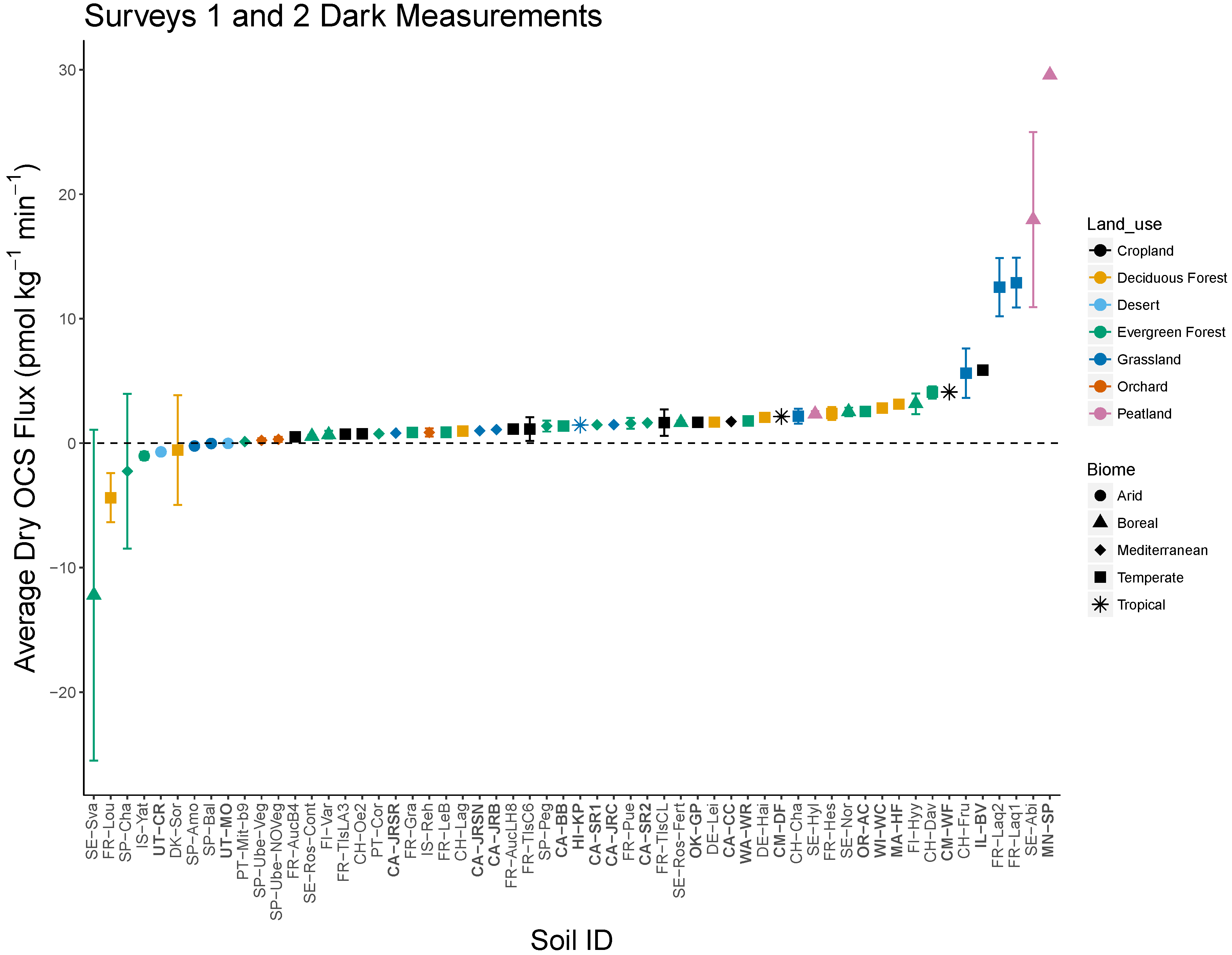
3.1. Patterns in OCS Production with Biome and Land Use

OCS production was widespread across a collection of diverse soils. The surveys included soils with diverse biome, land use, and physicochemical characteristics (

Table 3. Survey 1 and 2 site information and selected physicochemical properties sorted by biome and land use.

Survey 1
Soil ID	Latitude	Longitude	Biome	Land Use	pH	C/N	Clay (%)	Silt (%)	Sand (%)	MAT (°C)	MAP (mm)
UT-CR	38.68	−109.42	Arid	Desert	8.8	88	14	34	52	9.7	295
UT-MO	38.87	−109.81	Arid	Desert	9.4	172	36	58	6	10.9	225
CA-JRB	37.4	−122.23	Mediterranean	Grassland	7.5	12	11	37	52	14.6	618
CA-JRC	37.41	−122.23	Mediterranean	Grassland	7.3	11	11	39	50	14.6	618
CA-JRSN	37.41	−122.23	Mediterranean	Grassland	6.5	11	17	48	35	14.6	618
CA-JRSR	37.41	−122.23	Mediterranean	Grassland	7.4	12	10	43	47	14.6	618
CA-SR1	34.09	−118.66	Mediterranean	Evergreen Forest	7.3	21	13	36	51	14.8	450
CA-SR2	34.09	−118.66	Mediterranean	Evergreen Forest	7.6	17	8	33	59	14.8	450
CA-CC	37.43	−122.18	Mediterranean	Cropland	8.2	12	13	30	57	14.6	618
CA-BB	37.19	−122.22	Temperate	Evergreen Forest	6.4	25	10	36	54	14.6	618
OR-AC	42.18	−122.8	Temperate	Evergreen Forest	6.5	32	6	25	69	10.5	676
WA-WR	45.82	−121.95	Temperate	Evergreen Forest	5.3	33	1	4	95	8.4	1850
MA-HF	42.54	−72.17	Temperate	Deciduous Forest	4.3	21	4	26	70	8.8	1167
WI-WC	45.81	−90.08	Temperate	Deciduous Forest	5.8	15	3	15	82	4.7	812
IL-BV	40.01	−88.29	Temperate	Cropland	5.8	11	7	37	56	11.4	1013
OK-GP	36.61	−97.49	Temperate	Cropland	4.8	10	13	62	25	16.0	972
HI-KP	20.15	−155.83	Tropical	Grassland	6.6	10	7	26	67	20.3	2680
CM-DF	11.51	105.01	Tropical	Cropland	5.5	9	28	62	10	28.2	1453
CM-WF	11.51	105.01	Tropical	Cropland	4.6	10	25	59	16	28.2	1453
MN-SP	47.51	−93.45	Boreal	Peatland	4	33	n.d.	n.d.	n.d.	4.1	725
Survey 2
Soil ID	Latitude	Longitude	Biome	Land Use	pH	C/N	Clay (%)	Silt (%)	Sand (%)	MAT (°C)	MAP (mm)
SP-Amo	36.83	−2.25	Arid	Grassland	8.6	9	15	35	50	18.1	291
SP-Bal	39.94	−2.03	Arid	Grassland	8.4	19	18	28	54	13.8	427
IS-Yat	31.35	35.05	Arid	Evergreen Forest	8.1	30	29	49	22	21.0	217
IS-Reh	31.91	34.81	Mediterranean	Orchard	7.8	18	15	7	78	20.3	485
SP-Ube_NOVeg	37.92	−3.23	Mediterranean	Orchard	8.4	42	55	40	5	15.7	422
SP-Ube_Veg	37.91	−3.23	Mediterranean	Orchard	8.6	13	23	35	42	15.7	422
FR-Pue	43.74	3.6	Mediterranean	Evergreen Forest	6.9	18	42	32	26	13.8	755
PT-Cor	39.14	−8.33	Mediterranean	Evergreen Forest	5.7	18	4	16	80	16.7	811
PT-Mit-amb	38.54	−8	Mediterranean	Evergreen Forest	5.5	n.d.	n.d.	n.d.	n.d.	16.7	811
PT-Mit-b9	38.54	−8	Mediterranean	Evergreen Forest	5.9	18	4	9	87	16.7	811
PT-Mit-mid	38.54	−8	Mediterranean	Evergreen Forest	6	n.d.	n.d.	n.d.	n.d.	16.7	811
SP-Cha	40.65	0.21	Mediterranean	Evergreen Forest	5.5	19	13	20	67	15.3	490
SP-Peg	40.38	4.19	Mediterranean	Evergreen Forest	6.2	11	3	9	88	16.7	603
CH-Cha	47.21	8.41	Temperate	Grassland	6.3	27	28	44	28	9.5	1136
CH-Fru	47.12	8.54	Temperate	Grassland	4.9	10	42	47	11	9.2	1282
FR-Laq1	45.64	2.74	Temperate	Grassland	4.6	11	18	59	23	8.2	985
FR-Laq2	45.64	2.74	Temperate	Grassland	5.7	11	21	57	22	8.2	985
CH-Dav	46.81	9.86	Temperate	Evergreen Forest	4.3	25	22	25	53	2.6	2135
FR-Gra	44.76	0.6	Temperate	Evergreen Forest	4.6	27	4	5	91	13.2	794
FR-LeB	44.72	0.77	Temperate	Evergreen Forest	4.8	25	4	3	93	13.2	794
CH-Lag	47.12	8.54	Temperate	Deciduous Forest	6.3	13	42	43	15	9.2	1282
DE-Hai	51.08	10.45	Temperate	Deciduous Forest	6	13	48	49	4	8.6	672
DE-Lei	51.33	10.37	Temperate	Deciduous Forest	5.2	14	19	77	4	8.6	672
DK-Sor	55.49	11.64	Temperate	Deciduous Forest	4.2	19	15	23	62	9.0	584
FR_Rou	45.01	0.97	Temperate	Deciduous Forest	6.5	n.d.	n.d.	n.d.	n.d.	12.7	830
FR-Hes	48.67	7.07	Temperate	Deciduous Forest	5.4	14	24	61	15	10.3	743
FR-Lou	43.08	−0.04	Temperate	Deciduous Forest	7.9	23	14	38	48	12.8	845
CH-Oe2	47.29	7.73	Temperate	Cropland	7.3	10	42	47	11	9.1	1220
FR_TlsC6	43.54	1.51	Temperate	Cropland	8.6	22	18	35	47	13.9	660
FR_TlsLA3	43.53	1.5	Temperate	Cropland	8.5	15	28	45	27	13.9	660
FR-AucB4	43.62	0.57	Temperate	Cropland	8.4	30	33	49	18	13.9	712
FR-AucLH8	43.64	0.6	Temperate	Cropland	7.8	8	47	35	18	13.9	712
FR-TlsCL	43.53	1.51	Temperate	Cropland	5.7	8	33	42	25	13.9	660
SE-Abi	68.36	19.05	Boreal	Peatland	4.4	39	n.d.	n.d.	n.d.	−3.1	690
SE-Hyl	56.1	13.42	Boreal	Peatland	3.8	26	14	35	51	7.7	849
FI-Hyy	61.85	24.3	Boreal	Evergreen Forest	4.6	36	14	32	54	3.9	579
FI-Var	67.76	29.62	Boreal	Evergreen Forest	5.3	31	4	17	79	−0.6	578
SE-Nor	60.09	17.47	Boreal	Evergreen Forest	4.4	31	13	26	61	5.9	576
SE-Ros_Cont	64.17	19.75	Boreal	Evergreen Forest	5.2	41	4	15	81	2.0	635
SE-Ros_Fert	64.17	19.75	Boreal	Evergreen Forest	4.5	27	4	30	66	2.0	635
SE-Sva	64.17	19.78	Boreal	Evergreen Forest	4.7	47	9	28	63	2.0	635

n.d. not determined.

). Net emissions of OCS (positive flux) were observed in air-dried soils from approximately 90% of sites (51 of 58) from the two soil surveys in gas exchange rates measured in the dark at approximately 20 °C (20.5 °C for Survey 1; 17 °C for Survey 2). Under these conditions, OCS fluxes ranged in Survey 1 from −0.7 to 39.5 pmol (OCS) kg DW⁻¹ min^-1 with a median of 2.3 pmol(OCS) kg DW⁻¹ min⁻¹ and in Survey 2 site-averaged OCS fluxes ranged from −12.2 to 18.0 pmol(OCS) kg DW⁻¹ min⁻¹ with a median of 0.9 pmol(OCS) kg DW⁻¹ min⁻¹. The maximum emissions were observed in Boreal peatland samples for both surveys (MN-SP, SE-Abi). A minority of soils in both surveys exhibited net OCS uptake, although only one site with replicates was significantly different from zero (FR-Lou). A similar range of OCS fluxes was observed in both surveys (Figure 1) when considered under the same conditions (17 °C in the dark; Section 2.2.2). The remainder of the results are derived from independent statistical analyses of Surveys 1 and 2. This prevents differences in methods (Table 2) from affecting data interpretation and also allows us to determine whether results are consistent across what are essentially two separate studies.

Biome was a significant predictor variable for OCS fluxes in both surveys, and the patterns with biome were similar for the two surveys (

Table 4. The effect of biome and land use on Survey 1 OCS fluxes at 20 °C and 40 °C (F₂₀ and F₄₀, respectively) and temperature sensitivity (Q₁₀) and on Survey 2 F₂₀. The same within a column letter means no statistical difference (α = 0.05) between factor levels; factor levels with two letters means no statistical difference between factor levels with either letter. Survey 1 F₂₀ and F₄₀ were log transformed for analysis and back-transformed for presentation.

Effect	Survey 1			Survey 2
	F20	F40	Q10	F20
	ANOVA p-value
Biome	<0.001	<0.001	<0.001	<0.001
Land use	2	2	2	<0.001
Lsmeans	(pmol OCS kg−1 min−1)		-	(pmol OCS kg−1 min−1)
Arid	−0.46 B	0.44 C	1.65 C	−2.93 B
Mediterranean	1.73 A	8.74 B	2.66 B	0.38 AB
Boreal	3	3	3	0.59 AB
Temperate	3.44 A	21.48 A	2.83 AB	3.72 A
Tropical	3.37 A	23.90 A	3.18 A	1
Deciduous Forest	2	2	2	−2.02 B
Cropland	2	2	2	−1.62 B
Evergreen Forest	2	2	2	0.33 B
Orchard	1	1	1	0.84 AB
Grassland	2	2	2	4.64 A
Peatland	3	3	3	1
Desert	2	2	2	1

¹ not applicable to data set; ² not significant; ³ not included in analysis because of lack of variance.

) increasing from net OCS uptake (negative values) in arid soils to net OCS emission (positive) in all other soils in the following order: arid < Mediterranean < boreal < temperate < tropical soils. Differences were most significant at 40 °C (Table 4), where arid and Mediterranean soils were both significantly lower than temperate and tropical soils, although differences in production rates between the latter were not significant. Land use was a significant predictor variable for Survey 2, but not for Survey 1 in any model (p = 0.31 F₂₀; p = 0.19 F₄₀). Land use was significant in distinguishing grassland from deciduous and evergreen forests and cropland, but the orchards did not have significantly different F₂₀ from other land use types (Table 2).

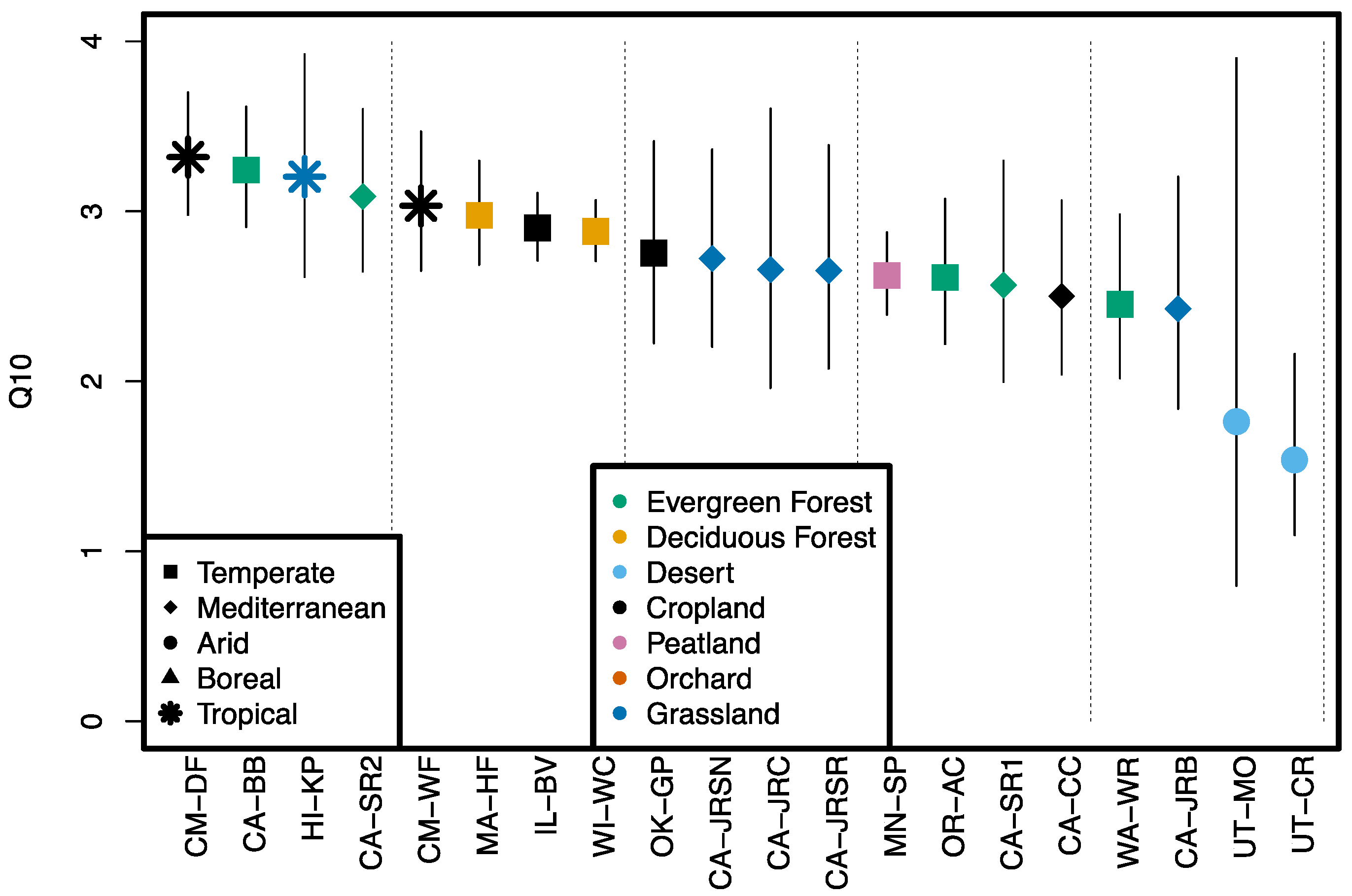
3.2. Temperature Response of OCS Production

Soil OCS emissions increased with temperature (15 to 40 °C) for all Survey 1 soils. Temperature sensitivity expressed as Q₁₀ varied between 1.54 and 3.32 and was on average 2.70 ± 0.21 (Figure 2) (±95% confidence intervals). Desert soils were net sinks of OCS at 20 °C and transitioned to sources of OCS at higher temperatures. Q₁₀ varied with biome (arid < Mediterranean < temperate < tropical) in the same order as OCS fluxes (see Section 3.1), and biome was a significant predictor variable distinguishing arid from Mediterranean and tropical soils, though temperate soils were not distinguishable from either Mediterranean or tropical soils (Table 4). Land use was not a significant predictor variable for temperature sensitivity (p = 0.81 Q₁₀).

3.3. Light Response of OCS Production

OCS emissions increased with light in most Survey 2 soils (33 out of 38). Light and dark OCS emissions were correlated (Pearson correlation; r = 0.89 p < 0.001), and OCS emissions in the light were 2.34 ± 0.06 times higher than in the dark (York fit linear slope [65]). However, the increase in temperature between light and dark treatments—a 6 °C change (from 17 to 23 °C)—can already explain a factor of 2 increase in OCS production for a Q₁₀ of 3 (i.e., 3^0.6~2). A linear model with conditioning (light vs. dark) as a fixed effect determined that conditioning was not a significant predictor (P = 0.12), and a linear model that used light sensitivity (i.e., light vs. dark conditioning) as the response variable was also run; neither biome nor land use were significant predictors (P = 0.48 and P = 0.9 respectively).

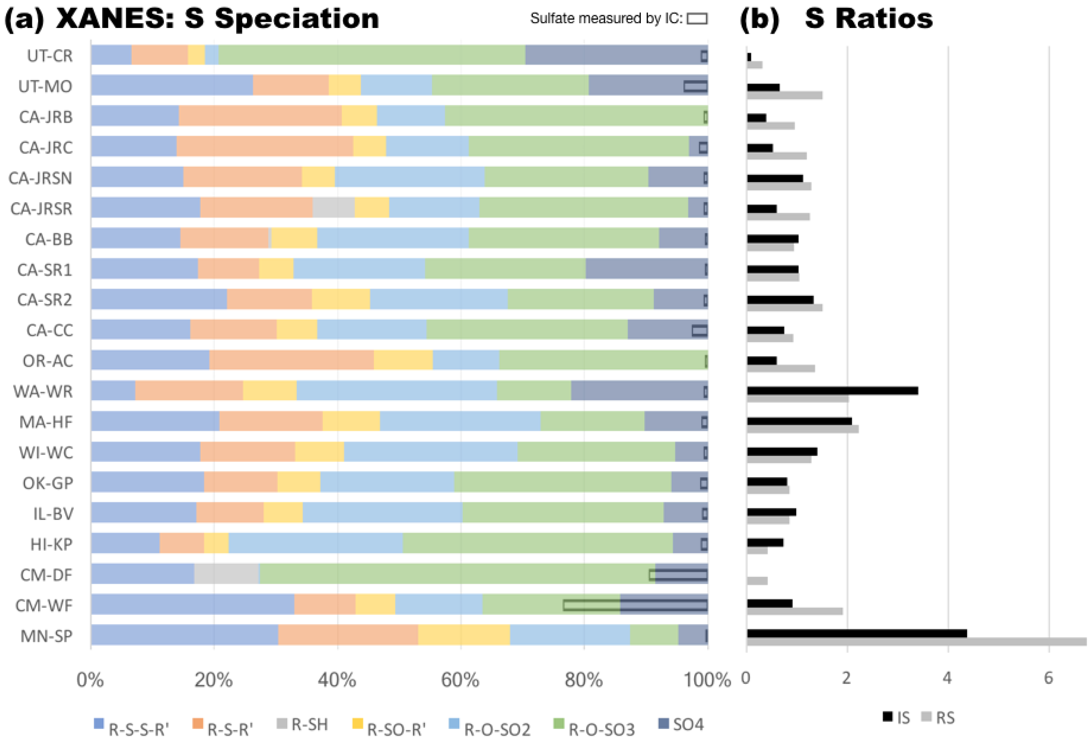
3.4. Soil Sulfur Speciation

The relative and absolute abundance of soil S species varied across the soils in Survey 1. Soil S ranged from 0.02 to 0.70% gS g DW⁻¹ with a median of 0.04% gS g DW⁻¹ (

Table 5. Selected soil S properties and stoichiometric ratios sorted by biome and land use (Survey 1).

Site	S (%)	C/N	C/S	N/S	P/S	SO4 (IC) (mg/kgS)
UT-CR	0.03	88	81	1	2	0.9
UT-MO	0.05	172	37	0	2	2.7
CA-JRB	0.02	12	67	6	1	0.3
CA-JRC	0.04	11	61	6	2	0.4
CA-JRSN	0.02	11	64	6	1	0.3
CA-JRSR	0.02	12	108	9	1	0.3
CA-BB	0.04	25	125	5	4	0.2
CA-SR1	0.04	21	41	2	3	0.2
CA-SR2	0.06	17	63	4	2	0.4
CA-CC	0.04	12	34	3	2	1.8
OR-AC	0.06	32	105	3	1	0.2
WA-WR	0.03	33	141	4	3	4.2
MA-HF	0.12	21	70	3	1	3.5
WI-WC	0.09	15	53	4	1	0.6
IL-BV	0.03	11	73	7	1	0.5
OK-GP	0.03	10	37	4	0	0.9
HI-KP	0.10	10	50	5	7	1.2
CM-DF	0.05	9	22	3	1	12.4
CM-WF	0.10	10	23	2	0	43.2
MN-SP	0.66	33	64	2	1	S 0.2

^S Total IC-derived sulfate listed, except where noted as soluble sulfate only.

). Soil S levels were exceptionally high in peat, which contained significant fractions of dead plant biomass (MN-SP). Most sulfur was present in the form of organic compounds in our soils. Inorganic sulfate (SO₄) was exceptionally high in tropical CM-WF soils (43.2% g(SO₄) gS⁻¹) and ranged from 0.2 and 12.4% g(SO₄) gS⁻¹ in the remaining soil samples, with a median of 0.6%. Adsorbed sulfate was present in six out of the eight soils with the highest soil sulfate levels, but the majority of soils (17 out of 20) had greater amounts of sulfate in water soluble than in the adsorbed phase.

We used bulk S K-edge XANES spectroscopy to determine the relative abundance of inorganic sulfate (SO₄) and organic compounds including organic disulfides (R-S-S-R’), organic sulfides (R-S-R’), thiols (R-SH), sulfoxides (R-SO-R’), sulfonates (R-O-SO₂), and organic sulfate (R-O-SO₃) (Figure 3a). Soil samples differed markedly in their sulfur speciation profiles, the highest proportion of organic sulfur on average was organic sulfate (31%), followed by organic sulfonate (19%), disulfide (18%), sulfide (15%), sulfoxide (7%), and thiol (1%). Inorganic sulfate concentrations determined by XANES and IC did not quantitatively agree (Figure 3a). This can primarily be attributed to uncertainty in XANES data, which are semi-quantitative for species classifications and may not reliably distinguish between sulfur species with very similar structure (e.g., organic and inorganic sulfate) in complex matrices, such as soil. We evaluated ratios of highly reduced organic S (RS) and intermediately oxidized organic S (RI) to highly oxidized organic S (RS = (R-S-S-R’ + R-S-R’ + R-SH)/R-O-SO₃; RI = (R-SO-R’ + R-O-SO₂)/R-O-SO₃) (Figure 3b). RS and RI were largest in peatland (MN-SP) and smallest in an arid (UT-CR) site, representing extremes in sulfur redox speciation (reduced and oxidized, respectively). S redox ratios were close to unity in most soils (1.2 for RS and 0.9 for RI in the median). Higher S redox ratios were found in some (e.g., WA-WR, MA-HF), but not all forests. Furthermore, S was more oxidized in the well-drained location (CM-DF) of the tropical agricultural site and more reduced in the water-logged location (CM-WF).

3.5. Sulfur Cycling in Soil Microbial Communities

Microbial function predicted from community composition of soils prior to drying may yield information regarding S compounds relevant to OCS production. We estimated the relative abundance of microbial S cycling pathways (see Section 2.3.1), including dissimilatory (e.g., sulfate reduction), assimilatory (e.g., cysteine biosynthesis), degradation (e.g., methionine degradation), and transport (e.g., sulfate transport) pathways. OCS production was correlated with the predicted prevalence of biosynthesis of S-containing amino acids such as cysteine (R-SH) and methionine (R-S-R’). PCA analysis of predicted microbial pathways (Figure 4) associated F₂₀, F₄₀, and Q₁₀ with the biosynthetic pathways for cysteine, methionine, thiamine (vitamin B1 synthesized from cysteine, S-containing pentane ring), and ethylene (by-product in methionine salvage pathway) along Dimension 2, which also separated sites by biome. Along Dimension 2, transport of methionine, glutathione (R-SH; essential S carrier in some organisms), and cystine (R-S-S-R’) and methionine degradation (to homocysteine, R-SH) also increased with OCS production, while methionine salvage (as opposed to degradation) decreased. OCS production terms were nearly orthogonal to sulfate cycling pathways, which were aligned with Dimension 1. This axis separated soils with high proportions of bacteria and sulfate reduction from those with relatively more eukaryotes and archaea, organic sulfur degradation, and sulfate transport. Cysteine biosynthesis by the two different pathways were orthogonal in the PCA, with alignment of bacterial cysteine biosynthesis from serine along Dimension 2 in contrast to fungal cysteine biosynthesis from homocysteine along Dimension 1. Soils from the Mediterranean biome were more similar in predicted S cycling than those collected from temperate biomes, which spanned the variance of Dimension 1.

In a complementary analysis, we recovered genes encoding for thiocyanate hydrolase (scnC) from soil metatranscriptomes from a subset of moist soil replicates from Survey 1 (Section 2.3.3). The results, including the frequency of assembled scnC genes per million genes in the transcriptomes, are presented in Appendix A. We did not observe a correlation between thiocyanate hydrolase (scnC) gene expression in moist soils (Table A1) and OCS production measured in soils following a median of 45 days of air drying.

3.6. Multivariate Analysis of Soil Factors Contributing to OCS Production

3.6.1. PLSR Models of Factors Driving F and Q₁₀

The cumulative amount of variance explained in the PLSR models of Survey 1 data was 0.58 for F₂₀, 0.63 for F₄₀, and 0.88 for Q₁₀. In all PLSR models (

Table 6. PLSR model summaries for Survey 1. OCS flux at 20 °C and 40 °C, and temperature sensitivity (Q₁₀). Weights were retained as ‘significant’ for squared values ≥ 0.05. The magnitude of the weight (w) of each predictor variable within each component (C1 and C2) show how much information is retained; predictors with the highest w can be interpreted as being drivers of the component. The +/− indicate the correlation relationship the predictor has with the response variable. Clr-transformed variables are labeled.

	Survey 1						Survey 2
	FOCS,20C		FOCS,40C		Q10		FOCS,20C
	C1 R2	C2 R2	C1 R2	C2 R2	C1 R2	C2 R2	C1 R2	C2 R2
	0.51	0.07	0.55	0.07	0.74	0.15	0.30	0.04
Predictors	C1 w	C2 w	C1 w	C2 w	C1 w	C2 w	C1 w	C2 w
BD	2	0.45	2	0.51	−0.24	2	1	1
pH	−0.49	2	−0.51	2	−0.39	2	−0.30	−0.29
Clay (clr)	2	2	2	2	2	0.26	2	−0.68
Silt (clr)	2	2	2	2	2	0.22	2	2
Sand (clr)	2	2	2	2	2	−0.25	2	0.45
GWC	2	2	2	2	0.22	2	1	1
Microbial C	0.22	−0.29	0.22	−0.29	2	−0.27	1	1
Microbial N	2	−0.29	2	−0.30	2	−0.28	1	1
C/N	−0.35	2	−0.30	2	−0.43	2	−0.46	2
C/S	2	2	2	2	2	−0.22	1	1
C (clr)	2	−0.26	2	2	2	−0.42	−0.44	0.23
N (clr)	0.34	2	0.30	−0.23	0.40	2	0.44	−0.23
P (clr)	−0.28	2	−0.28	2	2	2	1	1
K (clr)	2	0.35	2	0.30	−0.23	0.21	1	1
ISO4 (mg/kgS)	0.28	0.23	0.37	0.28	2	2	1	1
R-S-S-R’ (clr)	2	0.22	2	2	2	0.26	1	1
R-S-R’ (clr)	−0.24	−0.40	−0.27	−0.38	2	−0.30	1	1
R-SO-R’ (clr)	2	2	2	2	0.33	0.21	1	1
R-O-SO3 (clr)	−0.21	2	2	2	2	0.22	1	1
XSO4 (clr)	2	2	2	0.24	2	2	1	1
Redox	1	1	1	1	1	1	0.38	0.28
FCO2	1	1	1	1	1	1	2	2

¹ not applicable to data set; ² not significant; ^IIC- and ^XXANES-derived sulfate.

), the second component accounted for a much smaller amount of variance than the first component. In F models, significant weights (w) were relatively consistent between the first component of each model. The main driver (i.e., greatest absolute weight) of F in both Survey 1 models was pH, which had a negative association with the first component of each model. Positively associated drivers included N, SO₄, Microbial C, while other negatively associated drivers included C/N, P, and R-S-R’. BD and C were drivers of the second component, and S was never a significant driver. Drivers shared between F and Q₁₀ had the same sign and included pH, N, and C/N, but unlike F, Q₁₀ was negatively associated with BD (the main driver) and positively associated with R-SO-R’ in the first component, and to additional S species in the second component (Table 6). The cumulative amount of variance explained in the PLSR mode of Survey 2 was 0.34, less than was explained for Survey 1 (Table 6). Drivers were shared between the two surveys (including the direction of association) for pH, N, and C/N. In Survey 2, C emerged as a negatively associated driver, and redox (not measured in Survey 1) was a positively associated driver with the second greatest w (second to N).

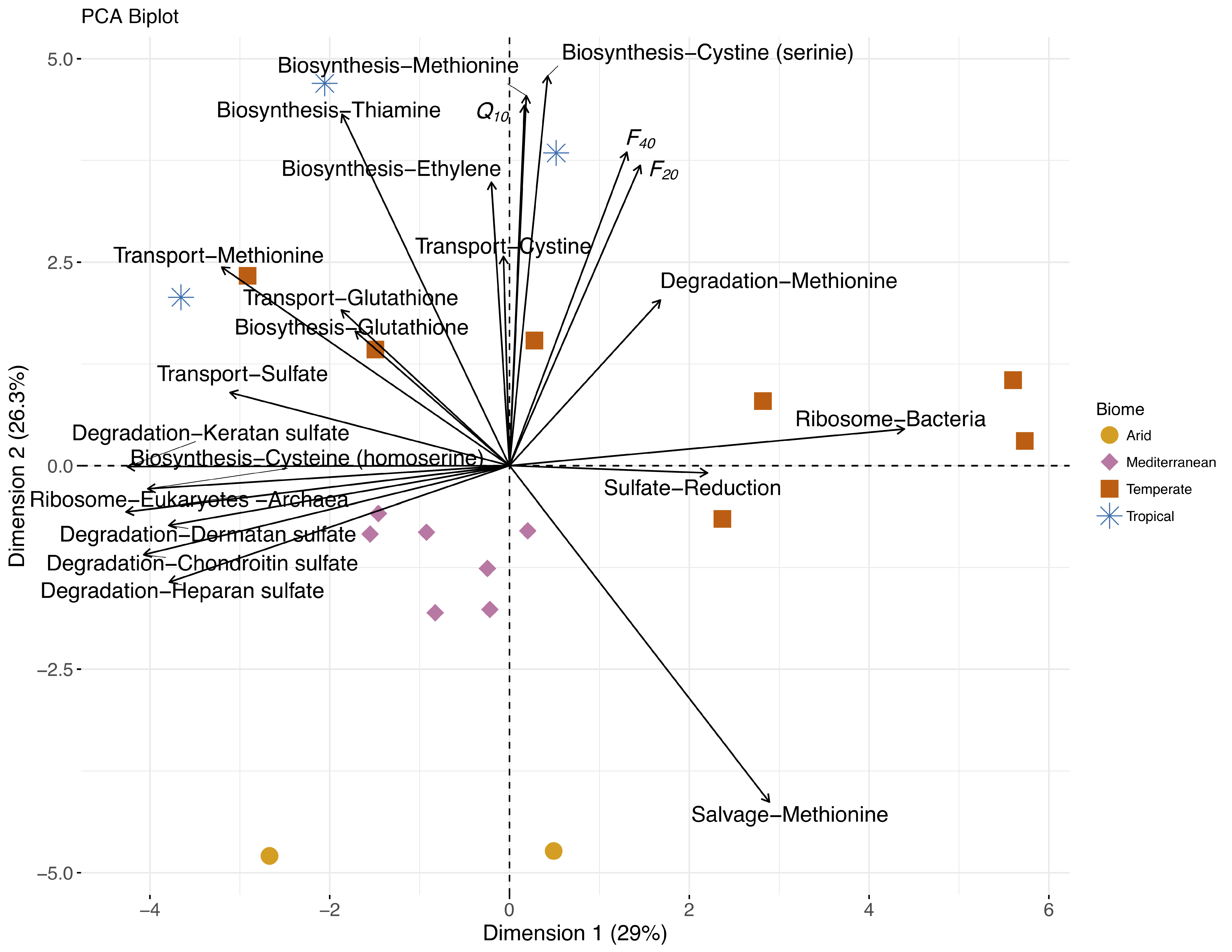
3.6.2. Integrated Analysis of Microbial and Chemical Factors Driving OCS Production

We evaluated correlations of soil properties with S XANES absorption spectra in each of 30 (0.5 eV) bins to assess patterns in S compounds, soil properties, and microbial pathways. This analysis complements results derived from direct comparison to XANES reference spectra (e.g., PLSR analysis in Table 6), as the correlation approach allows patterns to emerge through indirect comparison. Clustering patterns with soil properties and microbial pathways highlighted potentially relevant processes. Four clusters, characterized by sulfur redox state, emerged from the correlation analysis: (1) highly oxidized S, (2) broad range intermediate S redox states, (3) highly reduced S, and (4) intermediate S redox states emphasizing a narrow range in potential.

Reduced S regions of the XANES spectrum were associated with soil S, SO₄ (measured by IC), and sulfate reduction pathways (Cluster 3). These low energy regions may also include pyrite (FeS) and elemental sulfur, although their presence was not indicated when tested as reference species for this study. In contrast, highly oxidized XANES regions for inorganic and organic sulfate were associated with sulfate transport and pathways for sulfate acquisition (e.g., organic sulfate degradation) (Cluster 1), which were generally anti-correlated with availability of reduced S compounds such as S amino acids (Cluster 4). Variables associated with microbial diversity and abundance were most associated with a broad range of intermediate S (Cluster 2). Finally, a more narrow, intermediate range of S compounds were associated with biosynthetic pathways for cysteine (serine pathway; bacterial), methionine, ethylene, and thiamine, with F and Q₁₀, and with N/C and pH (Cluster 4). This narrow energy range (2479.75 to 2480.75 eV) is associated with sulfone reference compounds such as dibenzyl sulfonate [66].

4. Discussion

4.1. Ubiquitous OCS Production in Soils

OCS production is ubiquitous in dry soils, though may be masked at low temperatures in arid and alkaline soils by persistent OCS uptake. OCS production was widespread in our 58-site soil survey occurring in 84% of sites at temperatures between 17 °C and 20.5 °C in (Figure 1). Conversely, net OCS uptake was observed in nine dry soils. Three of these soils (SE-Sva, SP-Cha, DK-Sor) were also net CO₂ emitters, suggesting that microbial activity persisted in those soils, including respiration and potentially CA activity. Soil moisture was not determined after air drying in Survey 2, but the CO₂ fluxes may suggest that the soils were not sufficiently dried. In total, net CO₂ emissions were observed in 7 of 38 sites (F_CO2 > 0.1 µmol kg⁻² min⁻¹) but did not necessarily coincide with net uptake of OCS. Therefore, while F_CO2 may be a proxy for microbial activity in some soils, or even influence OCS fluxes [9], it was not a predictor of trends in dry OCS fluxes, as confirmed by the PLSR analysis (Table 6). The six other soils that took up OCS in Survey 2 and the two in Survey 1 shared the following characteristics: arid or temperate biomes, alkaline (pH between 7.9 and 9.4), and F_CO2 < 0. Alkaline and saline soils are known to exhibit net CO₂ uptake as a result of abiotic CO₂ dissolution, and in some cases leaching, of dissolved inorganic carbon [67], and rates of CA-catalyzed CO₂ hydration increase at high pH [47]. While we know that uncatalyzed OCS hydrolysis rates increase dramatically at high pH [47] and found that pH was the dominant driver for OCS production (Table 6), the pH-dependency of CA-catalyzed OCS uptake is not known. Survey 1 soils that took up OCS were very dry (e.g., 1.3% and 2.2% GWC for UT-CR and UT-MO, respectively), making it unlikely that microbial CA were active [10,13]. It is currently difficult to infer mechanisms regarding OCS uptake in dry soils from our understanding of soil CO₂ fluxes or soil CA activity. Even so, all Survey 1 soils produced OCS at high temperatures (Figure S1) suggesting that OCS production at low temperature was masked by OCS consumption. Correspondingly, we found that OCS production was a variable but ubiquitous process in soil.

4.2. Mechanisms of OCS Production in Soils

4.2.1. OCS Production from Thermal and Photo Degradation

Thermal degradation appears to be a key feature of soil OCS production, and variability in the degree of temperature sensitivity is related to soil properties. In recent work, the temperature sensitivity of OCS production determined from two-point temperature measurements in 27 moist soils (some identical samples to Survey 2) spanned a wide range of Q₁₀ values (from 0 to >7) with a mean and SD of 4.36 ± 4.45 [10]. Other studies have reported Q₁₀ values between 1.7 and 3.3 [7,8,11,68]. In our soils (Survey 1), Q₁₀ ranged from 1.54 to 3.32, and was on average 2.70 ± 0.21 (±95% confidence intervals). Two of the same sites used in Survey 1 were previously shown to have Q₁₀ values of 2.66 in air-dried soils (2.92 in this study) for IL-BV [8] and Q₁₀ values of 2.16 in dry soil (2.75 in this study) for OK-GP [7], and differences may be related to temporal or spatial variability, or differences in the range of temperatures use to determine Q₁₀. Soils with high N and RSOR and low pH, C/N, and BD had the highest Q₁₀ (Table 6), which is consistent with trends observed by PCA analysis (with N, pH, and BD) [10]. We showed that Q₁₀ may be associated with S compounds such as sulfones (R-O-SO₂) and either disulfides (R-S-S-R’), elemental sulfur, or pyrite (Figure 5). Thus, thermal sensitivity is an important property of soils to constrain for predicting variability in OCS production across ecosystems.

Photochemical degradation was a secondary process to thermal degradation under visible light, though UV-driven photochemical degradation is likely an important OCS production mechanism in the environment. OCS production from a variety of S compounds in aqueous systems depends on UV light (Table 1) and OCS production rates increase with decreasing wavelength [36,37]. In soils, OCS production rates were reported to increase in response to full spectrum light in incubations with stable temperature conditions (incandescent bulb; PAR 400–600 nm; 380 µmol(photons) m⁻² s⁻¹) [11]. In the present study, soil OCS production rates tended to increase in response to the light treatment in the visible range (400–700 nm with two weak peaks below 400 nm (UV); 580 µmol(photons) m⁻² s⁻¹), but the response was not significant. The apparent increase in OCS production rates in response to visible light can be attributed to the temperature artifact induced by the incubation lamps (see Section 2.2.3 and [13]). That is, the relative ratio of light/dark OCS production was 2.17 ± 0.39 (mean and 95% confidence intervals) can be explained by the expected temperature-induced ratio of 1.81 ± 0.08 determined from our Q₁₀ results (Survey 1) or ${1.70}_{-1.70}^{+1.48}$ that was calculated from independent measurements from some Survey 2 soils [10]. In the environment, solar irradiance drives important UV-driven photo-degradation reactions [69]. For example, OCS fluxes (emissions) in an alpine grassland were exponentially related to total incoming solar radiation (305 to 2800 nm), but only weakly related to modest changes in soil temperature (~10 °C) measured at 5 cm depth [5]. It may be difficult to attribute OCS production to either thermal or photo degradation reactions in the environment when solar radiation and temperature are highly correlated. For example, OCS production rates were exponentially related to air temperature at the OK-GP site (soil and senescing wheat material), which may also have been related to solar radiation [7]. We hypothesized that the dominant mechanism for OCS production in soils is abiotic photo-thermal degradation of S compounds. We confirmed that thermal degradation plays a dominant role in soils, but that photochemical degradation driven by visible light is insignificant. UV-driven photo-degradation reactions are likely important in the environment, but the remainder of our discussion focuses on non-photochemical mechanisms of soil OCS production that are most relevant to our results.

4.2.2. Direct Microbial OCS Production

Direct microbial production of OCS is likely minor compared to indirect production of OCS through the production of S-containing precursors by microbes. Direct OCS production has been observed in salt marsh environments, presumably mediated by saline microbial communities, which are typically less diverse and differ compositionally from soils [70]. Soil isolates, including common bacteria (e.g., Mycobacteria) and fungi (e.g., Ascomycota) may consume, and in some cases produce, OCS through unknown pathways [16,17,18]. Microbial OCS production via thiocyanate hydrolase and CS₂ hydrolase has been documented [71,72]. In this study, we evaluated thiocyanate hydrolase expressed in soils (see Appendix A) and have recently evaluated carbonic anhydrase gene expression [41]. Two roadblocks limit the conclusions we can draw from these data. Firstly, thiocyanate hydrolase and CS₂ hydrolase are enzymes that fall within broader enzyme classes (nitrile hydratase and β-class of CA, respectively). The distribution of OCS production across the significant genetic diversity within those classes is not known, but is critical for interpretation of genetic data, especially because β-CA are primarily known to take up (not produce) OCS. Secondly, RNA-based data collected from moist soils should not be expected to reflect microbial activity in soils that were additionally dried for ~45 days. Our metatranscriptome analysis does indicate that soil microbial communities have the genomic potential for thiocyanate hydrolase and CS₂ hydrolase activity, but stronger relationships cannot be inferred. In dry soils, microbial activity is limited by low moisture [42], although extracellular metabolic reactions may proceed with enzymes stabilized by soil particles [73]. In previous work, OCS production rates did not vary significantly between dry and moist soil [10], no temperature optimum (characteristic of enzyme activity) was observed (up to 68 °C in [8]), and OCS production persists following autoclaving [11,16]. Consistent with our expectations, we do not find evidence that direct microbial OCS production pathways contribute significantly to OCS fluxes in soils, though our current understanding of the populations and pathways involved in direct microbial OCS production is far from complete.

4.2.3. Precursors for OCS Production in Soils

Direct mechanisms connecting soil sulfate and OCS production are unclear, though soils high in sulfate and redox dynamics appear to promote OCS production. When measured by IC, sulfate was a driver of OCS production (Table 6) and was associated with reduced regions in the XANES sulfur spectrum associated with the sulfate reduction pathway (Figure 5c). However, the microbial pathway analysis found that the sulfate reduction pathway was orthogonal to OCS production rates (Figure 4). The role of sulfate was further complicated by inconsistent patterns in between the two analysis methods, IC and XANES (Figure 3), and by weak relationships between OCS and XANES sulfate levels. The relationship between sulfate and OCS production was primarily driven by the tropical soils from Cambodia (CM-WF and CM-DF; Figure 3a), which are seasonally flooded paddy soils (river water) for rice cultivation and are otherwise grazed. These conditions may induce particular S redox chemistry that is not linearly related to the other soils. In low sulfate soils, OCS production does not appear to be directly or mechanistically coupled to soil sulfate cycling, but connections may become important in soils with high levels of sulfate, potentially depending on redox dynamics.

Biological S assimilation and subsequent production of diverse organic S compounds is the source of a pool of OCS precursors in soil. We found that OCS production (both F and Q₁₀) was associated with cysteine, methionine, thiamine, and ethylene biosynthesis and cystine transport (Figure 4) and potentially a range of reduced and intermediate S compounds (Figure 5). Previous work has shown that S-containing amino acids cysteine (R-SH), methionine (R-S-R’), and related S compounds are OCS precursors (Table 1), and cysteine and thiocyanate additions to soil stimulate OCS production [74]. Approximately 11–31% of organic sulfur in soils is composed of cysteine and methionine (at about a 2:1 ratio), but these are difficult to independently and accurately measure [75]. S compound interconversions are complex and proceed quickly via biological (e.g., methionine salvage pathway [76]) and abiotic (e.g., cysteine oxidation to cystine [77]) pathways. The derivatives of cysteine and methionine span a broad range of S oxidation states that absorb energy from highly reduced (e.g., cystine (R-S-S-R’), the disulfide derivative of cysteine) to more intermediate (e.g., methionine sulfone (R-O-SO₂), an oxidized form of methionine) XANES spectral regions, consistent with the range of intermediate S redox states that were associated with OCS production terms (Figure 5c Cluster 4). If assimilated S compounds are precursors for OCS production, OCS precursors must be steadily produced or stabilized in soil to explain the long-lasting ability of dry soils to emit OCS (e.g., median 45 days for Survey 1). In aqueous systems, OCS precursor pools were finite, but relatively long lived as production rates from natural dissolved organic matter under UV light decreased only slowly over time [33]. Given enough time, OCS precursors may become depleted in dry or sterilized soils, and OCS emissions could cease until rewetting or recolonization. If this mechanism were important, it might help explain why arid-land soils exhibited the lowest OCS production rates (Table 4). Redox fluctuations that drive interconversions between S compounds may play an important role in fostering OCS precursor pools. Previous work has noted increases in OCS production at low redox potentials [47,78], consistent the expected low redox potential of CM soils, although we observed a positive relationship with redox potentials in Survey 2 (Table 6). Considering our results together with previous data, we propose that OCS emissions from soil arise from the production of organic S precursors during the biosynthesis of S-containing amino acids or other central S biomolecules such as thiamine and glutathione. These results are consistent with our hypothesis that plants and microbes may drive OCS production through indirect means.

4.3. Proposed OCS Production Mechanism of Coupled Biotic-Abiotic OCS Production from S-Containing Amino Acids

The results of our study suggest that a coupled abiotic-biotic mechanism drives OCS production in soils. Precursors for OCS emissions are produced in the course of microbial biosynthesis of S-containing amino acids cysteine and methionine and/or other central S biomolecules such as thiamine and glutathione. Direct precursor molecules may include these specific S compounds or their derivatives with S oxidation states around +II or lower. These OCS precursors maybe stabilized in microbial cells or in the soil matrix to facilitate relatively long-lasting OCS production potential from soils. We posit that direct OCS production from these chemical precursors is abiotic, and increases in response to temperature, and potentially light (although the UV light response was not evaluated in this study). This mechanism may be prevalent in both dry and moist soils. Differences in the amount or the availability of these precursors for degradation likely depends on properties of the soil such as total N content, C/N, pH, and BD either through direct effects or indirectly by affecting microbial activity and S cycling.

5. Conclusions

We have evaluated OCS production rates; their temperature and (visible) light sensitivity; and a wide range of soil chemical, physical, and microbial data for 58 soils collected in two distinct soil surveys. The evaluation revealed consistent patterns between soil S speciation and microbial S-cycling pathways, which we used to identify key processes driving OCS production, namely thermal degradation of chemical precursors produced as a consequence of microbial biosynthetic S pathways. We identified widespread microbial pathways that may play a role in returning OCS to the atmosphere from terrestrial ecosystems. This work provides mechanistic insight into the sources of OCS from soil that helps complete our understanding of a ubiquitous component of terrestrial OCS and S cycling.

5.1. Future Research Directions

Experimental evaluations of the sensitivity of soil OCS emission to UV light are now needed to better resolve the potential influence of solar radiation on OCS production mechanisms in various ecosystems. New efforts are needed to constrain the relationship between OCS production (or consumption) kinetics in microbial strains and genes encoding potentially related enzymes (e.g., thiocyanate and CS₂ hydrolase), and those efforts could be paired with quantification of production or consumption rates of those compounds in soils. The importance of plant-derived vs. microbe-derived OCS precursors to ecosystem OCS emissions is needed. These efforts will help outline the importance of land management practices use such as fertilizer addition and management of plant biomass for ecosystem OCS production.

The mechanistic relationships outlined in this paper will be helpful to modelers who aim to account for the contribution of soil OCS emissions in the OCS budget of the Earth’s atmosphere. OCS production rates must be constrained to accurately portray the OCS global atmospheric budget and apply OCS as a tracer for carbon cycling. Building from our results, modelers could predict spatial patterns of OCS production from microbial community data and predicted biosynthetic pathways. These data are becoming more prevalent and could be used to estimate activity on large scales [70,79]. Furthermore, maps of estimated OCS production rates and temperature sensitivity coefficients may be derived from relationships with soil edaphic factors (e.g., pH, N, and C/N) and/or trends with biome to improve model representations of soil OCS fluxes.

5.2. Outlook

OCS is the most abundant S-containing gas in the atmosphere, and resolving key components of the atmospheric budget, like soil OCS cycling, is important for understanding the global biogeochemical S cycle. Our results will provide new mechanistic insight into and predictive strategies for representing OCS production in soils. We are hopeful that these observations will be used to better represent soil OCS fluxes and improve the use of OCS as a tracer for leaf-level processes related to carbon and water cycling.

References

1. Kesselmeier, J.; Teusch, N.; Kuhn, U. Controlling variables for the uptake of atmospheric carbonyl sulfide by soil. Biogeochemistry 1999, 104, 11577–11584. [Google Scholar] [CrossRef] [Green Version]
2. Whelan, M.E.; Lennartz, S.T.; Gimeno, T.E.; Wehr, R.; Wohlfahrt, G.; Wang, Y.; Kooijmans, L.M.J.; Hilton, T.W.; Belviso, S.; Peylin, P.; et al. Reviews and Syntheses: Carbonyl Sulfide as a Multi-scale Tracer for Carbon and Water Cycles. Biogeosci. Discuss. 2017, 1–97. [Google Scholar] [CrossRef] [Green Version]
3. Commane, R.; Meredith, L.K.; Baker, I.T.; Berry, J.A.; Munger, J.W.; Montzka, S.A.; Templer, P.H.; Juice, S.M.; Zahniser, M.S.; Wofsy, S.C. Seasonal fluxes of carbonyl sulfide in a midlatitude forest. Proc. Natl. Acad. Sci. USA 2015, 112, 14162–14167. [Google Scholar] [CrossRef] [PubMed]
4. Billesbach, D.P.; Berry, J.A.; Seibt, U.; Maseyk, K.; Torn, M.S.; Fischer, M.L.; Abu-Naser, M.; Campbell, J.E. Growing season eddy covariance measurements of carbonyl sulfide and CO2 fluxes: COS and CO2 relationships in Southern Great Plains winter wheat. Agric. For. Meteorol. 2014, 184, 48–55. [Google Scholar] [CrossRef]
5. Kitz, F.; Gerdel, K.; Hammerle, A.; Laterza, T.; Spielmann, F.M.; Wohlfahrt, G. In situ soil COS exchange of a temperate mountain grassland under simulated drought. Oecologia 2017, 183, 851–860. [Google Scholar] [CrossRef] [PubMed] [Green Version]
6. Sun, W.; Maseyk, K.; Lett, C.; Seibt, U. Litter dominates surface fluxes of carbonyl sulfide in a Californian oak woodland. J. Geophys. Res. Biogeosci. 2016, 121, 438–450. [Google Scholar] [CrossRef] [Green Version]
7. Maseyk, K.; Berry, J.A.; Billesbach, D.; Campbell, J.E.; Torn, M.S.; Zahniser, M.; Seibt, U. Sources and sinks of carbonyl sulfide in an agricultural field in the Southern Great Plains. Proc. Natl. Acad. Sci. USA 2014, 111, 9064–9069. [Google Scholar] [CrossRef] [PubMed]
8. Whelan, M.E.; Hilton, T.W.; Berry, J.A.; Berkelhammer, M.; Desai, A.R.; Campbell, J.E. Carbonyl sulfide exchange in soils for better estimates of ecosystem carbon uptake. Atmos. Chem. Phys. 2016, 16, 3711–3726. [Google Scholar] [CrossRef]
9. Bunk, R.; Behrendt, T.; Yi, Z.; Andreae, M.O.; Kesselmeier, J. Exchange of carbonyl sulfide (OCS) between soils and atmosphere under various CO2 concentrations. J. Geophys. Res. Biogeosci. 2017, 122, 1343–1358. [Google Scholar] [CrossRef]
10. Kaisermann, A.; Ogée, J.; Sauze, J.; Wohl, S.; Jones, S.P.; Gutierrez, A.; Wingate, L. Disentangling the rates of carbonyl sulphide (COS) production and consumption and their dependency with soil properties across biomes and land use types. Atmos. Chem. Phys. Discuss. 2018, 1–27. [Google Scholar] [CrossRef] [Green Version]
11. Whelan, M.E.; Rhew, R.C. Carbonyl sulfide produced by abiotic thermal and photodegradation of soil organic matter from wheat field substrate. J. Geophys. Res. Biogeosci. 2015, 120, 54–62. [Google Scholar] [CrossRef] [Green Version]
12. Fried, A.; Klinger, L.F.; Erickson, D.J. Atmospheric carbonyl sulfide exchange in bog microcosms. Geophys. Res. Lett. 1993, 20, 129–132. [Google Scholar] [CrossRef]
13. Gimeno, T.E.; Ogée, J.; Royles, J.; Gibon, Y.; West, J.B.; Burlett, R.; Jones, S.P.; Sauze, J.; Wohl, S.; Benard, C.; et al. Bryophyte gas-exchange dynamics along varying hydration status reveal a significant carbonyl sulphide (COS) sink in the dark and COS source in the light. New Phytol. 2017, 215, 965–976. [Google Scholar] [CrossRef] [PubMed] [Green Version]
14. Berry, J.; Wolf, A.; Campbell, J.E.; Baker, I.; Blake, N.; Blake, D.; Denning, A.S.; Kawa, S.R.; Montzka, S.A.; Seibt, U.; et al. A coupled model of the global cycles of carbonyl sulfide and CO2: A possible new window on the carbon cycle. J. Geophys. Res. Biogeosci. 2013, 118, 842–852. [Google Scholar] [CrossRef]
15. Sauze, J.; Ogée, J.; Maron, P.A.; Crouzet, O.; Nowak, V.; Wohl, S.; Kaisermann, A.; Jones, S.P.; Wingate, L. The interaction of soil phototrophs and fungi with pH and their impact on soil CO2, CO18O and OCS exchange. Soil Biol. Biochem. 2017, 115, 371–382. [Google Scholar] [CrossRef] [PubMed]
16. Kato, H.; Saito, M.; Nagahata, Y.; Katayama, Y. Degradation of ambient carbonyl sulfide by Mycobacterium spp. in soil. Microbiology 2008, 154, 249–255. [Google Scholar] [CrossRef] [PubMed] [Green Version]
17. Masaki, Y.; Ozawa, R.; Kageyama, K.; Katayama, Y. Degradation and emission of carbonyl sulfide, an atmospheric trace gas, by fungi isolated from forest soil. FEMS Microbiol. Lett. 2016, 363. [Google Scholar] [CrossRef] [PubMed]
18. Ogawa, T.; Kato, H.; Higashide, M.; Nishimiya, M.; Katayama, Y. Degradation of carbonyl sulfide by Actinomycetes and detection of clade D of β-class carbonic anhydrase. FEMS Microbiol. Lett. 2016, 363, fnw223. [Google Scholar] [CrossRef] [PubMed]
19. Smith, N.A.; Kelly, D.P. Oxidation of Carbon Disulphide as the Sole Source of Energy for the Autotrophic Growth of Thiobacillus thioparus Strain TK-m. Microbiology 1988, 134, 3041–3048. [Google Scholar] [CrossRef] [Green Version]
20. Sorokin, D.Y.; Abbas, B.; van Zessen, E.; Muyzer, G. Isolation and characterization of an obligately chemolithoautotrophic Halothiobacillus strain capable of growth on thiocyanate as an energy source. FEMS Microbiol. Lett. 2014, 354, 69–74. [Google Scholar] [CrossRef] [PubMed] [Green Version]
21. Ogawa, T.; Noguchi, K.; Saito, M.; Nagahata, Y.; Kato, H.; Ohtaki, A.; Nakayama, H.; Dohmae, N.; Matsushita, Y.; Odaka, M.; et al. Carbonyl Sulfide Hydrolase from Thiobacillus thioparus Strain THI115 Is One of the β-Carbonic Anhydrase Family Enzymes. J. Am. Chem. Soc. 2013, 135, 3818–3825. [Google Scholar] [CrossRef] [PubMed]
22. Bezsudnova, E.Y.; Sorokin, D.Y.; Tikhonova, T.V.; Popov, V.O. Thiocyanate hydrolase, the primary enzyme initiating thiocyanate degradation in the novel obligately chemolithoautotrophic halophilic sulfur-oxidizing bacterium Thiohalophilus thiocyanoxidans. Biochim. Biophys. Acta Proteins Proteom. 2007, 1774, 1563–1570. [Google Scholar] [CrossRef] [PubMed]
23. Hussain, A.; Ogawa, T.; Saito, M.; Sekine, T.; Nameki, M.; Matsushita, Y.; Hayashi, T.; Katayama, Y. Cloning and expression of a gene encoding a novel thermostable thiocyanate-degrading enzyme from a mesophilic alphaproteobacteria strain THI201. Microbiology 2013, 159, 2294–2302. [Google Scholar] [CrossRef] [PubMed] [Green Version]
24. Katayama, Y.; Narahara, Y.; Inoue, Y.; Amano, F.; Kanagawa, T.; Kuraishi, H. A thiocyanate hydrolase of Thiobacillus thioparus. A novel enzyme catalyzing the formation of carbonyl sulfide from thiocyanate. J. Biol. Chem. 1992, 267, 9170–9175. [Google Scholar] [PubMed]
25. Yamasaki, M.; Matsushita, Y.; Nyunoya, H.; Katayama, Y.; Namura, M. Genetic and Immunochemical Characterization of Thiocyanate-Degrading Bacteria in Lake Water Genetic and Immunochemical Characterization of Thiocyanate-Degrading Bacteria in Lake Water. Appl. Environ. Microbiol. 2002, 68, 942–946. [Google Scholar] [CrossRef] [PubMed]
26. Welte, C.U.; Rosengarten, J.F.; de Graaf, R.M.; Jetten, M.S.M. SaxA-Mediated Isothiocyanate Metabolism in Phytopathogenic Pectobacteria. Appl. Environ. Microbiol. 2016, 82, 2372–2379. [Google Scholar] [CrossRef] [PubMed] [Green Version]
27. Churka Blum, S.; Lehmann, J.; Solomon, D.; Caires, E.F.; Alleoni, L.R.F. Sulfur forms in organic substrates affecting S mineralization in soil. Geoderma 2013, 200–201, 156–164. [Google Scholar] [CrossRef]
28. Kertesz, M.A.; Mirleau, P. The role of soil microbes in plant sulphur nutrition. J. Exp. Bot. 2004, 55, 1939–1945. [Google Scholar] [CrossRef] [PubMed] [Green Version]
29. Minami, K.; Fukushi, S. Volatilization of carbonyl sulfide from paddy soils treated with sulfur-containing substances. Soil Sci. Plant Nutr. 1981, 27, 339–345. [Google Scholar] [CrossRef] [Green Version]
30. Lehmann, S.; Conrad, R. Characteristics of Turnover of Carbonyl Sulfide in 4 Different Soils. J. Atmos. Chem. 1996, 23, 193–207. [Google Scholar] [CrossRef]
31. Hanschen, F.S.; Lamy, E.; Schreiner, M.; Rohn, S. Reactivity and Stability of Glucosinolates and Their Breakdown Products in Foods. Angew. Chem. Int. Ed. 2014, 53, 11430–11450. [Google Scholar] [CrossRef] [PubMed]
32. Steiger, A.K.; Zhao, Y.; Pluth, M.D. Emerging Roles of Carbonyl Sulfide in Chemical Biology: Sulfide Transporter or Gasotransmitter? Antioxid. Redox Signal. 2017. [Google Scholar] [CrossRef] [PubMed]
33. Ferek, R.J.; Andreae, M.O. Photochemical production of carbonyl sulphide in marine surface waters. Nature 1984, 307, 148–150. [Google Scholar] [CrossRef]
34. Flöck, O.R.; Andreae, M.O.; Dräger, M. Environmentally relevant precursors of carbonyl sulfide in aquatic systems. Mar. Chem. 1997, 59, 71–85. [Google Scholar] [CrossRef]
35. Kelly, D.P.; Wood, A.P.; Jordan, S.L.; Padden, A.N.; Gorlenko, V.M.; Dubinina, G.A. Biological production and consumption of gaseous organic sulphur compounds. Biochem. Soc. Trans. 1994, 22, 1011–1015. [Google Scholar] [CrossRef] [PubMed] [Green Version]
36. Zepp, R.G.; Andreae, M.O. Factors affecting the photochemical production of carbonyl sulfide in seawater. Geophys. Res. Lett. 1994, 21, 2813–2816. [Google Scholar] [CrossRef]
37. Du, Q.; Mu, Y.; Zhang, C.; Liu, J.; Zhang, Y.; Liu, C. Photochemical production of carbonyl sulfide, carbon disulfide and dimethyl sulfide in a lake water. J. Environ. Sci. 2017, 51, 146–156. [Google Scholar] [CrossRef] [PubMed]
38. Geng, C.; Mu, Y. Carbonyl sulfide and dimethyl sulfide exchange between trees and the atmosphere. Atmos. Environ. 2006, 40, 1373–1383. [Google Scholar] [CrossRef] [Green Version]
39. Zhang, L.; Walsh, R.S.; Cutter, G.A. Estuarine cycling of carbonyl sulfide: Production and sea–air flux. Mar. Chem. 1998, 61, 127–142. [Google Scholar] [CrossRef]
40. Pos, W.H.; Riemer, D.D.; Zika, R.G. Carbonyl sulfide (OCS) and carbon monoxide (CO) in natural waters: Evidence of a coupled production pathway. Mar. Chem. 1998, 62, 89–101. [Google Scholar] [CrossRef]
41. Meredith, L.K.; Ogée, J.; Boye, K.; Singer, E.; Wingate, L.; von Sperber, C.; Sengupta, A.; Whelan, M.; Pang, E.; Keiluweit, M.; et al. Soil exchange rates of COS and CO18O shift with the diversity of microbial communities and their carbonic anhydrase enzymes. ISME J. 2018, in press. [Google Scholar]
42. Tecon, R.; Or, D. Biophysical processes supporting the diversity of microbial life in soil. FEMS Microbiol. Rev. 2017, 41, 599–623. [Google Scholar] [CrossRef] [PubMed] [Green Version]
43. Hobbie, S. Chloroform Fumigation Direct Extraction (CFDE) Protocol for Microbial Biomass Carbon and Nitrogen. Allison Lab Protoc. 2008, 4. [Google Scholar]
44. Brookes, P.C.; Landman, A.; Pruden, G.; Jenkinson, D.S. Chloroform fumigation and the release of soil nitrogen: A rapid direct extraction method to measure microbial biomass nitrogen in soil. Soil Biol. Biochem. 1985, 17, 837–842. [Google Scholar] [CrossRef]
45. Vance, E.D.; Brookes, P.C.; Jenkinson, D.S. Microbial biomass measurements in forest soils: The use of the chloroform fumigation-incubation method in strongly acid soils. Soil Biol. Biochem. 1987, 19, 697–702. [Google Scholar] [CrossRef]
46. Kooijmans, L.M.J.; Uitslag, N.A.M.; Zahniser, M.S.; Nelson, D.D.; Montzka, S.A.; Chen, H. Continuous and high precision atmospheric concentration measurements of COS, CO2, CO and H2O using a quantum cascade laser spectrometer (QCLS). Atmos. Meas. Tech. Discuss. 2016, 9, 5293–5314. [Google Scholar] [CrossRef]
47. Ogée, J.; Sauze, J.; Kesselmeier, J.; Genty, B.; Van Diest, H.; Launois, T.; Wingate, L. A new mechanistic framework to predict OCS fluxes from soils. Biogeosciences 2016, 13, 2221–2240. [Google Scholar] [CrossRef] [Green Version]
48. Fierer, N.; Schimel, J.P. Effects of drying-rewetting frequency on soil carbon and nitrogen transformations. Soil Biol. Biochem. 2002, 34, 777–787. [Google Scholar] [CrossRef]
49. Di Stefano, C.; Ferro, V.; Mirabile, S. Comparison between grain-size analyses using laser diffraction and sedimentation methods. Biosyst. Eng. 2010, 106, 205–215. [Google Scholar] [CrossRef]
50. Harris, I.; Jones, P.D.; Osborn, T.J.; Lister, D.H. Updated high-resolution grids of monthly climatic observations—The CRU TS3.10 Dataset. Int. J. Climatol. 2014, 34, 623–642. [Google Scholar] [CrossRef] [Green Version]
51. Jalilehvand, F. Sulfur: Not a “silent” element any more. Chem. Soc. Rev. 2006, 35, 1256–1268. [Google Scholar] [CrossRef] [PubMed]
52. Ravel, B.; Newville, M. ATHENA, ARTEMIS, HEPHAESTUS: Data analysis for X-ray absorption spectroscopy using IFEFFIT. J. Synchrotron Radiat. 2005, 12, 537–541. [Google Scholar] [CrossRef] [PubMed]
53. Beck, T.; Joergensen, R.G.; Kandeler, E.; Makeshin, E.; Nuss, E.; Oberholzer, H.R.; Scheu, S. An inter-laboratory comparison of ten different ways of measuring soil microbial biomass C. Soil Biol. Biochem. 1997, 29, 1023–1032. [Google Scholar] [CrossRef]
54. Ward, T. BugBase predicts organism-level microbiome phenotypes. bioRxiv 2017, 1–36. [Google Scholar] [CrossRef]
55. Kanehisa, M.; Furumichi, M.; Tanabe, M.; Sato, Y.; Morishima, K. KEGG: New perspectives on genomes, pathways, diseases and drugs. Nucleic Acids Res. 2017, 45, D353–D361. [Google Scholar] [CrossRef] [PubMed]
56. Kanehisa, M.; Sato, Y.; Kawashima, M.; Furumichi, M.; Tanabe, M. KEGG as a reference resource for gene and protein annotation. Nucleic Acids Res. 2016, 44, D457–D462. [Google Scholar] [CrossRef] [PubMed]
57. Ogata, H.; Goto, S.; Sato, K.; Fujibuchi, W.; Bono, H.; Kanehisa, M. KEGG: Kyoto encyclopedia of genes and genomes. Nucleic Acids Res. 1999, 27, 29–34. [Google Scholar] [CrossRef] [PubMed]
58. Chen, I.M.A.; Markowitz, V.M.; Chu, K.; Palaniappan, K.; Szeto, E.; Pillay, M.; Ratner, A.; Huang, J.; Andersen, E.; Huntemann, M.; et al. IMG/M: Integrated genome and metagenome comparative data analysis system. Nucleic Acids Res. 2017, 45, D507–D516. [Google Scholar] [CrossRef] [PubMed]
59. Wattam, A.R.; Abraham, D.; Dalay, O.; Disz, T.L.; Driscoll, T.; Gabbard, J.L.; Gillespie, J.J.; Gough, R.; Hix, D.; Kenyon, R.; et al. PATRIC, the bacterial bioinformatics database and analysis resource. Nucleic Acids Res. 2014, 42, D581–D591. [Google Scholar] [CrossRef] [PubMed]
60. Langille, M.G.I.; Zaneveld, J.; Caporaso, J.G.; McDonald, D.; Knights, D.; Reyes, J.A.; Clemente, J.C.; Burkepile, D.E.; Vega Thurber, R.L.; Knight, R.; et al. Predictive functional profiling of microbial communities using 16S rRNA marker gene sequences. Nat. Biotechnol. 2013, 31, 814–821. [Google Scholar] [CrossRef] [PubMed] [Green Version]
61. Katayama, Y.; Matsushita, Y.; Kaneko, M.; Kondo, M.; Mizuno, T.; Nyunoya, H. Cloning of genes coding for the three subunits of thiocyanate hydrolase of Thiobacillus thioparus THI 115 and their evolutionary relationships to nitrile hydratase. J. Bacteriol. 1998, 180, 2583–2589. [Google Scholar] [PubMed]
62. Abdi, H. Partial least squares regression and projection on latent structure regression (PLS Regression). Wiley Interdiscip. Rev. Comput. Stat. 2010, 2, 97–106. [Google Scholar] [CrossRef]
63. Carrascal, L.M.; Galván, I.; Gordo, O. Partial least squares regression as an alternative to current regression methods used in ecology. Oikos 2009, 118, 681–690. [Google Scholar] [CrossRef] [Green Version]
64. Aitchison, J. The Statistical Analysis of Compositional Data, Monographs on Statistics and Applied Probability; Chapman and Hall: London, UK, 1986. [Google Scholar]
65. Wehr, R.; Saleska, S.R. The long-solved problem of the best-fit straight line: Application to isotopic mixing lines. Biogeosciences 2017, 14, 17–29. [Google Scholar] [CrossRef]
66. Manceau, A.; Nagy, K.L. Quantitative analysis of sulfur functional groups in natural organic matter by XANES spectroscopy. Geochim. Cosmochim. Acta 2012, 99, 206–223. [Google Scholar] [CrossRef]
67. Ma, J.; Wang, Z.-Y.; Stevenson, B.A.; Zheng, X.-J.; Li, Y. An inorganic CO2 diffusion and dissolution process explains negative CO2 fluxes in saline/alkaline soils. Sci. Rep. 2013, 3, 2025. [Google Scholar] [CrossRef] [PubMed]
68. Saito, M.; Honna, T.; Kanagawa, T.; Katayama, Y. Microbial Degradation of Carbonyl Sulfide in Soils. Microbes Environ. 2002, 17, 32–38. [Google Scholar] [CrossRef] [Green Version]
69. Baker, N.R.; Allison, S.D.; Frey, S.D. Ultraviolet photodegradation facilitates microbial litter decomposition in a Mediterranean climate. Ecology 2015, 96, 1994–2003. [Google Scholar] [CrossRef] [PubMed] [Green Version]
70. Thompson, L.R.; Sanders, J.G.; McDonald, D.; Amir, A.; Ladau, J.; Locey, K.J.; Prill, R.J.; Tripathi, A.; Gibbons, S.M.; Ackermann, G.; et al. A communal catalogue reveals Earth’s multiscale microbial diversity. Nature 2017, 551, 457–463. [Google Scholar] [CrossRef] [PubMed]
71. Katayama, Y.; Kanagawa, T.; Kuraishi, H. Emission of Carbonyl Sulfide by Thiobacillus-Thioparus Grown with Thiocyanate in Pure and Mixed Cultures. FEMS Microbiol. Lett. 1993, 114, 223–228. [Google Scholar] [CrossRef]
72. Smeulders, M.J.; Pol, A.; Venselaar, H.; Barends, T.R.M.; Hermans, J.; Jetten, M.S.M.; Op den Camp, H.J.M. Bacterial CS2 hydrolases from Acidithiobacillus thiooxidans strains are homologous to the archaeal catenane CS2 hydrolase. J. Bacteriol. 2013, 195, 4046–4056. [Google Scholar] [CrossRef] [PubMed]
73. Wang, B.; Lerdau, M.; He, Y. Widespread production of nonmicrobial greenhouse gases in soils. Glob. Chang. Biol. 2017, 23, 4472–4482. [Google Scholar] [CrossRef] [PubMed]
74. Minami, K.; Fukushi, S. Detection of carbonyl sulfide among gases produced by the decomposition of cystine in paddy soils. Soil Sci. Plant Nutr. 1981, 27, 105–109. [Google Scholar] [CrossRef] [Green Version]
75. Morra, M.J.; Dick, W.A. Production of Thiocysteine (Sulfide) in Cysteine Amended Soils. Soil Sci. Soc. Am. J. 1985, 49, 882–886. [Google Scholar] [CrossRef]
76. Sekowska, A.; Dénervaud, V.; Ashida, H.; Michoud, K.; Haas, D.; Yokota, A.; Danchin, A. Bacterial variations on the methionine salvage pathway. BMC Microbiol. 2004, 4, 1–17. [Google Scholar] [CrossRef] [PubMed] [Green Version]
77. Freney, J.R. Aerobic transformation of cysteine to sulphate in soil. Nature 1958, 182, 1318–1319. [Google Scholar] [CrossRef]
78. Devai, I.; DeLaune, R.D. Formation of volatile sulfur compounds in salt marsh sediment as influenced by soil redox condition. Org. Geochem. 1995, 23, 283–287. [Google Scholar] [CrossRef]
79. Delgado-Baquerizo, M.; Oliverio, A.M.; Brewer, T.E.; Benavent-González, A.; Eldridge, D.J.; Bardgett, R.D.; Maestre, F.T.; Singh, B.K.; Fierer, N. A global atlas of the dominant bacteria found in soil. Science 2018, 359, 320–325. [Google Scholar] [CrossRef] [PubMed]
Figure 1. Net OCS soil fluxes from two independent soil surveys measured at approximately 17 °C in the dark in Survey 1 (bold text) and Survey 2 (normal text). Survey 1 fluxes at 17 °C were estimated from measured fluxes at 20.5 °C using the temperature sensitivity for each soil. Site biome is indicated by symbol type and land use by color. Error bars represent standard deviation of three soil replicates measured in Survey 2. Positive OCS fluxes indicate emissions of OCS from soils, while negative fluxes indicate net OCS uptake.
Soilsystems 02 00037 g001
Figure 2. OCS production temperature sensitivity (Q10) for Survey 1 soils observed over temperature ramp between 15 °C and 40 °C in the dark. Site biome is indicated by symbol type and land use by color. Error bars indicate upper and lower 95% confidence intervals on exponential fit.
Soilsystems 02 00037 g002
Figure 3. Soil sulfur speciation (Survey 1). For each site, (a) relative proportion of sulfur species (% total S) as measured by XANES (solid bars) and compared with total sulfate measured by IC (right-justified outline bars); and (b) S species ratios including (RS) highly reduced to highly oxidized (grey bars) and (IS) intermediate oxidized to highly oxidized (black bars). Sites ordered as in Table 5.
Soilsystems 02 00037 g003
Figure 4. Patterns of relatedness of S-cycling pathways and ribosomal phenotypes for each sample site PCA of predicted microbial sulfur pathways for each site (points; color indicates biome, symbol indicates land use). Arrows denote the projection of pathways (similar pathways marked by same color) and OCS fluxes and temperature sensitivity onto Dimension 1 (29%) and Dimension 2 (26.3%).
Soilsystems 02 00037 g004
Figure 5. Comparison of site-level trends in XANES absorption spectra with soil physical, chemical, and microbial parameters. S XANES K-edge absorption spectra averaged in 0.5 eV bins (2470 to 2486 eV region) for (a) samples and (b) reference compounds. (c) Correlation coefficient heatmap (Pearson’s product moment) between 0.5 eV bins average XANES absorption (columns) and soil chemical, physical, or microbial parameter (rows) and across 19 soil sites (MN-SP soils excluded). Clustering performed using Ward’s D2 method (R package pheatmap). Asterisks denote coefficients significantly different from zero (p-value < 0.05). The negative of the correlation for pH shown.
Soilsystems 02 00037 g005