
Cosmic Ray Muon Navigation for Subsurface Environments: Technologies and Challenges


Abstract
1. Introduction
2. Muon Physical Properties
2.1. Observed Muon Flux
2.2. Energy-Loss Models
3. Muon Measurements
3.1. Detectors
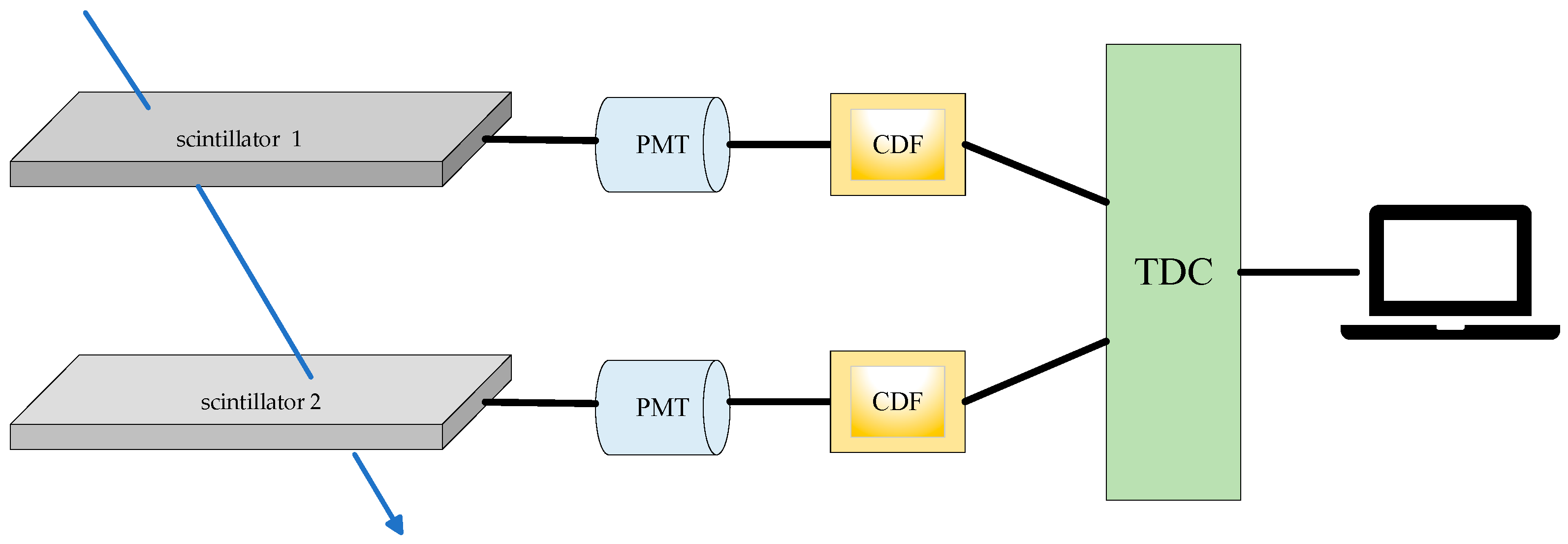
3.2. Time of Flight
3.3. Incident Coordinates
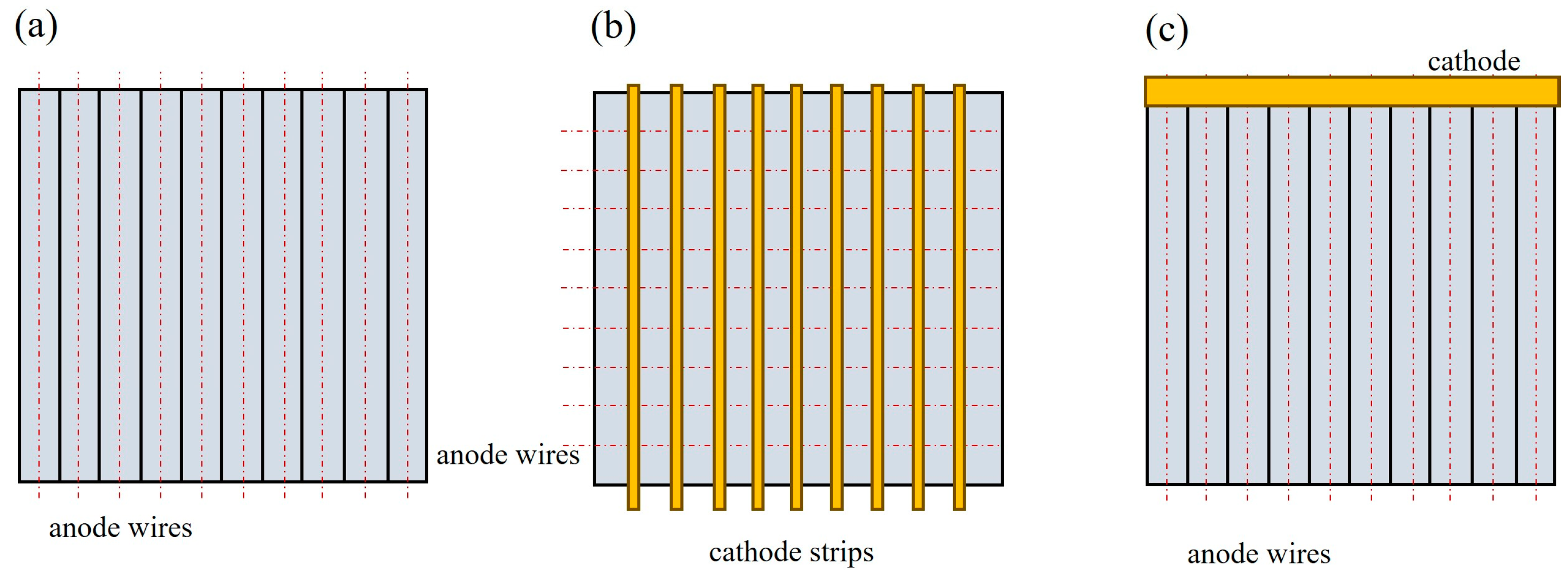
3.3.1. Gaseous Detectors
3.3.2. Scintillation Detectors
3.3.3. Other Detectors
4. Muon Navigation
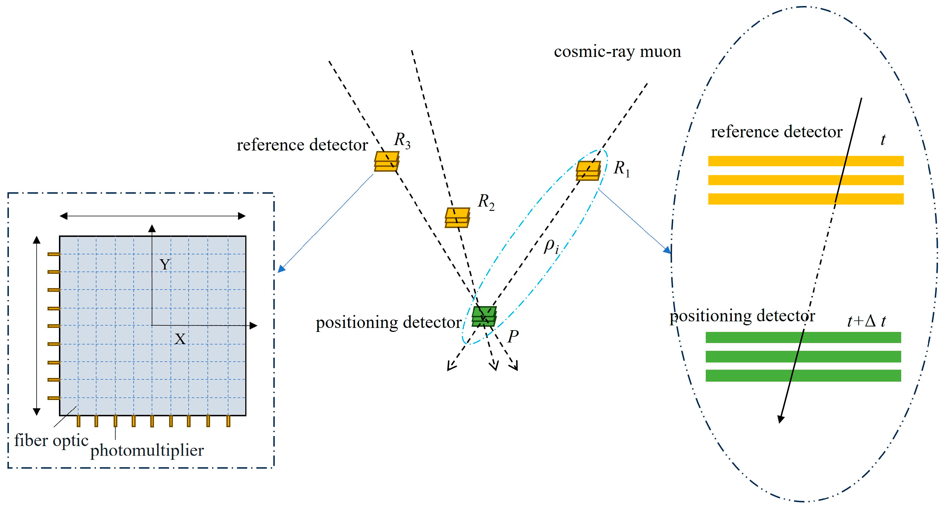
4.1. Positioning Principle
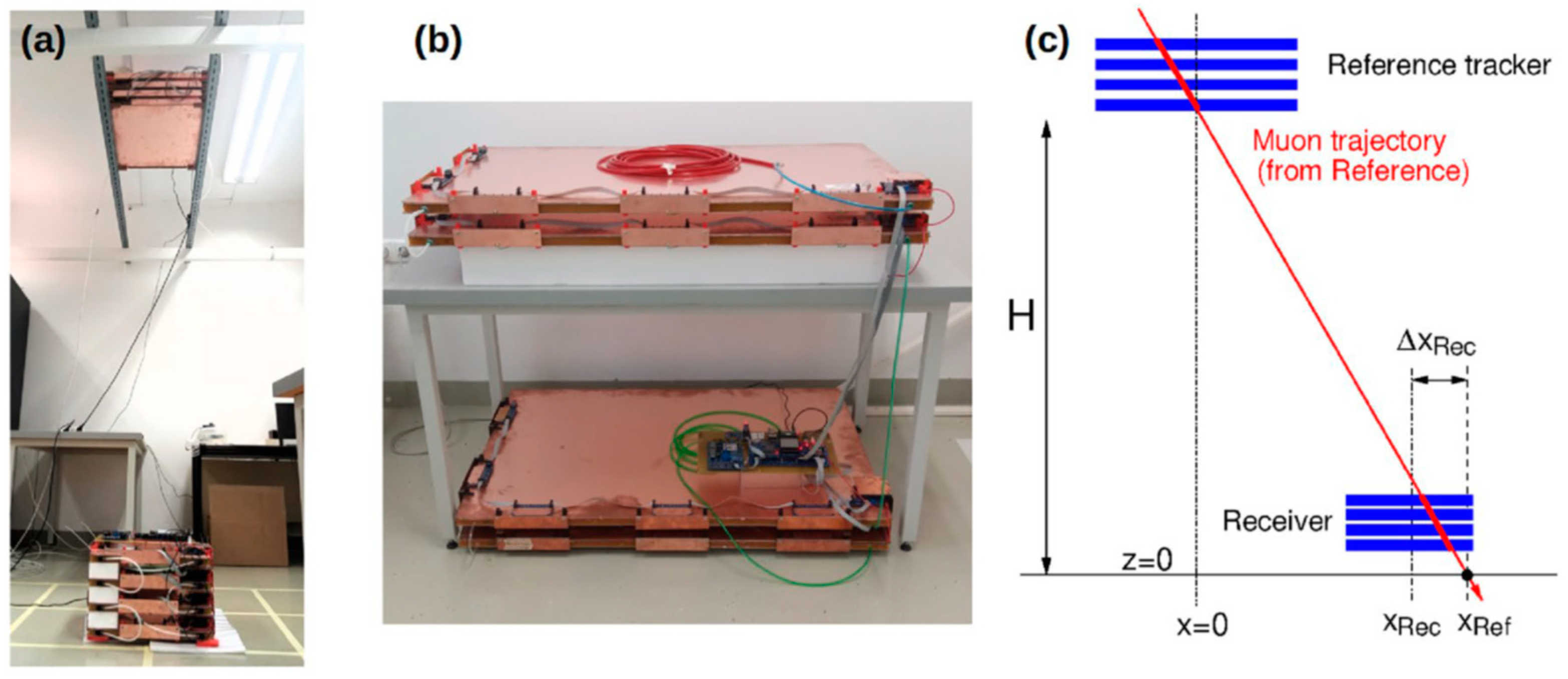
4.2. Current Achievements
5. Challenges
5.1. Navigation Signals
5.2. Positioning Models
5.3. Application Scenarios
6. Conclusions
Author Contributions
Funding
Conflicts of Interest
References
- Sakpere, W.; Adeyeye-Oshin, M.; Mlitwa, N. A state-of-the-art survey of indoor positioning and navigation systems and technologies. S. Afr. Comput. J. 2017, 29, 145–197. [Google Scholar] [CrossRef]
- Aparicio, J.; Álvarez, F.J.; Hernández, Á.; Holm, S. A survey on acoustic positioning systems for location-based services. IEEE Trans. Instrum. Meas. 2022, 71, 8505336. [Google Scholar] [CrossRef]
- Tiemann, J.; Schweikowski, F.; Wietfeld, C. Design of an UWB indoor-positioning system for UAV navigation in GNSS-denied environments. In Proceedings of the 2015 International Conference on Indoor Positioning and Indoor Navigation (IPIN), Banff, AB, Canada, 13–16 October 2015; IEEE: Piscataway, NJ, USA, 2015; pp. 1–7. [Google Scholar] [CrossRef]
- Zhang, H.; Ye, C. A visual positioning system for indoor blind navigation. In Proceedings of the 2020 IEEE International Conference on Robotics and Automation (ICRA), Paris, France, 31 May–31 August 2020; IEEE: Piscataway, NJ, USA, 2020; pp. 9079–9085. [Google Scholar] [CrossRef]
- Ruan, Y.; Chen, L.; Zhou, X.; Liu, Z.; Liu, X.; Guo, G.; Chen, R. iPos-5G: Indoor positioning via commercial 5G NR CSI. IEEE Internet Things J. 2022, 10, 8718–8733. [Google Scholar] [CrossRef]
- Zhao, H.; Zhang, N.; Xu, L.; Lin, P.; Liu, Y.; Li, X. Summary of research on geomagnetic navigation technology. IOP Conf. Ser. Earth Environ. Sci. 2021, 769, 032031. [Google Scholar] [CrossRef]
- Javed, W.; Ghani, S.; Elmqvist, N. Gravnav: Using a gravity model for multi-scale navigation. In Proceedings of the International Working Conference on Advanced Visual Interfaces, Naples, Italy, 22–25 May 2012; pp. 217–224. [Google Scholar] [CrossRef]
- Yang, Y.; Xu, T.; Xue, S. Progresses and Prospects in Developing Marine Geodetic Datum and Marine Navigation of China. Acta Geod. Cartogr. Sin. 2017, 46, 1–8. [Google Scholar] [CrossRef]
- Boguspayev, N.; Akhmedov, D.; Raskaliyev, A.; Kim, A.; Sukhenko, A. A comprehensive review of GNSS/INS integration techniques for land and air vehicle applications. Appl. Sci. 2023, 13, 4819. [Google Scholar] [CrossRef]
- Kim, Y.; Hwang, D.H. Vision/INS integrated navigation system for poor vision navigation environments. Sensors 2016, 16, 1672. [Google Scholar] [CrossRef]
- Liu, P.; Wang, B.; Deng, Z.; Fu, M. INS/DVL/PS tightly coupled underwater navigation method with limited DVL measurements. IEEE Sens. J. 2018, 18, 2994–3002. [Google Scholar] [CrossRef]
- Yang, C.; Cheng, Z.; Jia, X.; Zhang, L.; Li, L.; Zhao, D. A novel deep learning approach to 5g csi/geomagnetism/vio fused indoor localization. Sensors 2023, 23, 1311. [Google Scholar] [CrossRef]
- Yang, Y. Concepts of comprehensive PNT and related key technologies. Acta Geod. Cartogr. Sin. 2016, 45, 505–510. [Google Scholar] [CrossRef]
- Marteau, J.; Gibert, D.; Lesparre, N.; Nicollin, F.; Noli, P.; Giacoppo, F. Muons tomography applied to geosciences and volcanology. Nucl. Instrum. Methods Phys. Res. Sect. A Accel. Spectrometers Detect. Assoc. Equip. 2012, 695, 23–28. [Google Scholar] [CrossRef]
- Del Santo, M.; Catalano, O.; Cusumano, G.; La Parola, V.; La Rosa, G.; Maccarone, M.C.; Mineo, T.; Sottile, G.; Carbone, D.; Zuccarello, L.; et al. Looking inside volcanoes with the imaging atmospheric Cherenkov telescopes. Nucl. Instrum. Methods Phys. Res. Sect. A Accel. Spectrometers Detect. Assoc. Equip. 2017, 876, 111–114. [Google Scholar] [CrossRef]
- D’Alessandro, R.; Ambrosino, F.; Baccani, G.; Bonechi, L.; Bongi, M.; Caputo, A.; Ciaranfi, R.; Cimmino, L.; Ciulli, V.; D’Errico, M.; et al. Volcanoes in Italy and the role of muon radiography. Philos. Trans. R. Soc. A 2019, 377, 20180050. [Google Scholar] [CrossRef] [PubMed]
- Ebisuzaki, T.; Miyahara, H.; Kataoka, R. Explosive volcanic eruptions triggered by cosmic rays: Volcano as a bubble chamber. Gondwana Res. 2011, 19, 1054–1061. [Google Scholar] [CrossRef]
- Oláh, L.; Tanaka, H.K.M. Machine learning with muographic images as input: An application to volcano eruption forecasting. In Muography: Exploring Earth’s Subsurface with Elementary Particles; AGU Publications: Malden, MA, USA, 2022; pp. 43–54. [Google Scholar] [CrossRef]
- Tanaka, H. Muography for a dense tide monitoring network. Sci. Rep. 2022, 12, 6725. [Google Scholar] [CrossRef]
- Gómez, H. Muon tomography using micromegas detectors: From Archaeology to nuclear safety applications. Nucl. Instrum. Methods Phys. Res. Sect. A Accel. Spectrometers Detect. Assoc. Equip. 2019, 936, 14–17. [Google Scholar] [CrossRef]
- Berns, H.; Burnett, T.; Gran, R.; Wilkes, R. GPS time synchronization in school-network cosmic ray detectors. IEEE Trans. Nucl. Sci. 2004, 51, 848–853. [Google Scholar] [CrossRef]
- Tanaka, H. Cosmic time synchronizer (CTS) for wireless and precise time synchronization using extended air showers. Sci. Rep. 2022, 12, 7078. [Google Scholar] [CrossRef]
- Morishima, K.; Kuno, M.; Nishio, A.; Kitagawa, N.; Manabe, Y.; Moto, M.; Takasaki, F.; Fujii, H.; Satoh, K.; Kodama, H.; et al. Discovery of a big void in Khufu’s Pyramid by observation of cosmic-ray muons. Nature 2017, 552, 386–390. [Google Scholar] [CrossRef]
- Su, N.; Liu, Y.-Y.; Wang, L.; Cheng, J.-P. Muon radiography simulation for underground palace of Qinshihuang Mausoleum. Acta Phys. Sin. 2021, 71, 330–336. [Google Scholar] [CrossRef]
- Liu, G.; Luo, X.; Tian, H.; Yao, K.; Niu, F.; Jin, L.; Gao, J.; Rong, J.; Fu, Z.; Kang, Y.; et al. High-precision muography in archaeogeophysics: A case study on Xi’an defensive walls. J. Appl. Phys. 2023, 133, 014901. [Google Scholar] [CrossRef]
- Tanaka, H.; Bozza, C.; Bross, A.; Cantoni, E.; Catalano, O.; Cerretto, G.; Giammanco, A.; Gluyas, J.; Gnesi, I.; Holma, M.; et al. Muography. Nat. Rev. Methods Primers 2023, 3, 88. [Google Scholar] [CrossRef]
- Tanaka, H. Muometric positioning system (μPS) with cosmic muons as a new underwater and underground positioning technique. Sci. Rep. 2020, 10, 18896. [Google Scholar] [CrossRef] [PubMed]
- Tanaka, H. Wireless muometric navigation system. Sci. Rep. 2022, 12, 10114. [Google Scholar] [CrossRef]
- Tanaka, H.; Gallo, G.; Gluyas, J.; Kamoshida, O.; Lo Presti, D.; Shimizu, T.; Steigerwald, S.; Takano, K.; Yang, Y.; Yokota, Y.; et al. First navigation with wireless muometric navigation system (MuWNS) in indoor and underground environments. iScience 2023, 26, 107000. [Google Scholar] [CrossRef]
- Tanaka, H. Muometric positioning system (muPS) utilizing direction vectors of cosmic-ray muons for wireless indoor navigation at a centimeter-level accuracy. Sci. Rep. 2023, 13, 15272. [Google Scholar] [CrossRef]
- Tanaka, H. Cosmic-ray arrival time (CAT) indoor navigation in the World Geodetic System. Res. Square. 2024, preprint. [Google Scholar] [CrossRef]
- Varga, D.; Tanaka, H. Developments of a centimeter-level precise muometric wireless navigation system (MuWNS-V) and its first demonstration using directional information from tracking detectors. Sci. Rep. 2024, 14, 7605. [Google Scholar] [CrossRef]
- Xiong, K.; Wei, C.; Zhou, P. Research on underwater positioning method based on cosmic muons detection. Tactical Missile Technol. 2023, 4, 56–68. [Google Scholar] [CrossRef]
- Yang, Y.; Ren, X. Muometric navigation with cosmic muon-ray. J. Navig. Position. 2023, 11, 8–13. [Google Scholar] [CrossRef]
- Li, H.; Zhang, C.; Fan, X.; Tian, L.; Li, T.; Pang, Y.; Yang, Y. A muon high-resolution pseudorange measurement method: Application to muon navigation in confined spaces. Chin. J. Aeronaut. 2024, 37, 391–404. [Google Scholar] [CrossRef]
- Wang, Y.; Liu, J.; Yang, L.; Zeng, Z.; Ma, H.; Yue, Q. Jinping Underground Laboratory and Rare Physics Experiments in China. Nucl. Tech. 2023, 46, 173–181. [Google Scholar] [CrossRef]
- Bonomi, G.; Checchia, P.; D’Errico, M.; Pagano, D.; Saracino, G. Applications of cosmic-ray muons. Prog. Part. Nucl. Phys. 2020, 112, 103768. [Google Scholar] [CrossRef]
- Agafonova, N.; Alexandrov, A.; Anokhina, A.; Aoki, S.; Ariga, A.; Ariga, T.; Bertolin, A.; Bozza, C.; Brugnera, R.; Buonaura, A.; et al. Measurement of the cosmic ray muon flux seasonal variation with the OPERA detector. J. Cosmol. Astropart. Phys. 2019, 2019, 003. [Google Scholar] [CrossRef]
- Enqvist, T.; Mattila, A.; Föhr, V.; Jämsén, T.; Lehtola, M.; Narkilahti, J.; Joutsenvaara, J.; Nurmenniemi, S.; Peltoniemi, J.; Remes, H.; et al. Measurements of muon flux in the Pyhäsalmi underground laboratory. Nucl. Instrum. Methods Phys. Res. Sect. A Accel. Spectrometers Detect. Assoc. Equip. 2005, 554, 286–290. [Google Scholar] [CrossRef]
- Bergamasco, L.; Bilokon, H.; Piazzoli, B.; Mannocchi, G.; Castagnoli, C.; Picchi, P. Deep underground multiple muons at the Mt. Blanc station. Nuovo C. Lett. 1979, 26, 609–614. [Google Scholar] [CrossRef]
- Guo, Z.; Bathe-Peters, L.; Chen, S.; Chouaki, M.; Dou, W.; Guo, L.; Hussain, G.; Li, J.-J.; Liu, Q.; Luo, G.; et al. Muon flux measurement at china jinping underground laboratory. Chin. Phys. C 2021, 45, 025001. [Google Scholar] [CrossRef]
- Stockel, C.T. A study of muons deep underground. I. Angular distribution and vertical intensity. J. Phys. A Gen. Phys. 1969, 2, 639. [Google Scholar] [CrossRef]
- Gray, F.; Ruybal, C.; Totushek, J.; Mei, D.-M.; Thomas, K.; Zhang, C. Cosmic ray muon flux at the Sanford Underground Laboratory at Homestake. Nucl. Instrum. Methods Phys. Res. Sect. A Accel. Spectrometers Detect. Assoc. Equip. 2011, 638, 63–66. [Google Scholar] [CrossRef]
- Esch, E.; Bowles, T.; Hime, A.; Pichlmaier, A.; Reifarth, R.; Wollnik, H. The cosmic ray muon flux at WIPP. Nucl. Instrum. Methods Phys. Res. Sect. A Accel. Spectrometers Detect. Assoc. Equip. 2005, 538, 516–525. [Google Scholar] [CrossRef]
- Zhang, C.; Mei, D. Measuring muon-induced neutrons with liquid scintillation detector at Soudan mine. Phys. Rev. D 2014, 90, 122003. [Google Scholar] [CrossRef]
- Robinson, M.; Kudryavtsev, V.A.; Lüscher, R.; McMillan, J.E.; Lightfoot, P.K.; Spooner, N.J.C.; Smith, N.J.T.; Liubarsky, I. Measurements of muon flux at 1070m vertical depth in the Boulby underground laboratory. Nucl. Instrum. Methods Phys. Res. Sect. A Accel. Spectrometers Detect. Assoc. Equip. 2003, 511, 347–353. [Google Scholar] [CrossRef]
- Bellini, G.; Benziger, J.; Bick, D.; Bonfini, G.; Bravo, D.; Buizza Avanzini, M.; Caccianiga, B.; Cadonati, L.; Calaprice, F.; Carraro, C.; et al. Cosmic-muon flux and annual modulation in Borexino at 3800 m water-equivalent depth. J. Cosmol. Astropart. Phys. 2012, 2012, 015. [Google Scholar] [CrossRef]
- Cherry, M.; Deakyne, M.; Lande, K.; Lee, C.K.; Steinberg, R.I.; Cleveland, B.; Fenyves, E.J. Multiple muons in the Homestake underground detector. Phys. Rev. D Part. Fields Gravit. Cosmol./Phys. Rev. D Part. Fields 1983, 27, 1444–1447. [Google Scholar] [CrossRef]
- Formaggio, J. Measurement of Atmospheric Neutrinos at the Sudbury Neutrino Observatory. Nucl. Phys. Sect. A 2009, 827, 498c–500c. [Google Scholar] [CrossRef]
- Mei, D.; Hime, A. Muon-induced background study for underground laboratories. Phys. Rev. D—Part. Fields Gravit. Cosmol. 2006, 73, 053004. [Google Scholar] [CrossRef]
- Fedynitch, A.; Woodley, W.; Piro, M.C. On the accuracy of underground muon intensity calculations. Astrophys. J. 2022, 928, 27. [Google Scholar] [CrossRef]
- Bonechi, L.; Bongi, M.; Fedele, D.; Grandi, M.; Ricciarini, S.; Vannuccini, E. Development of the ADAMO detector: Test with cosmic rays at different zenith angles. In Proceedings of the 29th International Cosmic Ray Conference, Pune, India, 3–10 August 2005; pp. 283–286. [Google Scholar]
- Heck, D.; Knapp, J.; Capdevielle, J.N.; Schatz, G.; Thouw, T. CORSIKA: A Monte Carlo Code to Simulate Extensive Air Showers; Forschungszentrum Karlsruhe GmbH: Karlsruhe, Germany, 1998. [Google Scholar]
- Gaisser, T.; Ralph, E.; Elisa, R. Cosmic Rays and Particle Physics; Cambridge University Press: Cambridge, UK, 1990. [Google Scholar]
- Tang, A.; Horton-Smith, G.; Kudryavtsev, V.; Tonazzo, A. Muon simulations for super-kamiokande, kamland, and chooz. Phys. Rev. D—Part. Fields Gravit. Cosmol. 2006, 74, 053007. [Google Scholar] [CrossRef]
- Bugaev, E.; Misaki, A.; Naumov, V.; Sinegovskaya, T.S.; Sinegovsky, S.I.; Takahashi, N. Atmospheric muon flux at sea level, underground, and underwater. Physical Review D 1998, 58, 054001. [Google Scholar] [CrossRef]
- Pagano, D.; Bonomi, G.; Donzella, A.; Zenoni, A.; Zumerle, G.; Zurlo, N. EcoMug: An Efficient Cosmic Muon Generator for cosmic-ray muon applications. Nucl. Instrum. Methods Phys. Res. Sect. A Accel. Spectrometers Detect. Assoc. Equip. 2021, 1014, 165732. [Google Scholar] [CrossRef]
- Woodley, W.; Fedynitch, A.; Piro, M.C. Cosmic ray muons in laboratories deep underground. Phys. Rev. D 2024, 110, 063006. [Google Scholar] [CrossRef]
- Procureur, S. Muon imaging: Principles, technologies and applications. Nucl. Instrum. Methods Phys. Res. Sect. A Accel. Spectrometers Detect. Assoc. Equip. 2018, 878, 169–179. [Google Scholar] [CrossRef]
- Li, Y.; Wang, G.; Xu, X.; Feng, L.; Wang, C. Geophysical application of cosmic-ray muon detection technology. Prog. Geophys. 2021, 36, 0753–0758. [Google Scholar] [CrossRef]
- Bethe, H. Zur Theorie des Durchgangs schneller Korpuskularstrahlen durch Materie. Ann. Der Phys. 1930, 397, 325–428. [Google Scholar] [CrossRef]
- Tanabashi, M.; Hagiwara, K.; Hikasa, K.; Nakamura, K.; Sumino, Y.; Takahashi, F.; Tanaka, J.; Agashe, K.; Alielli, G.; Amsler, C.; et al. Review of Particle Physics: Particle data groups. Phys. Rev. D 2018, 98, 1–1898. [Google Scholar] [CrossRef]
- Groom, D.E.; Mokhov, N.V.; Striganov, S.I. Muon stopping power and range tables 10 MeV–100 TeV. At. Data Nucl. Data Tables 2001, 78, 183–356. [Google Scholar] [CrossRef]
- Ye, B.; Li, Y.; Zhou, Z. Muon imaging and elemental analysis. Physics 2021, 50, 248–256. [Google Scholar] [CrossRef]
- Wang, J.; Bu, Z.; Wang, Z.; Xu, J.; Zhou, L.; Zheng, Q. A High Precision Time Measurement Method Based on Phase-Fitting for Muon Detection. arXiv 2024, arXiv:2411.08408. [Google Scholar]
- Augusto, C.; Navia, C.; Lopes do Valle, R.; da Silva, T.F. Digital signal processing for time of flight measurements of muons at sea level. Nucl. Instrum. Methods Phys. Res. Sect. A Accel. Spectrometers Detect. Assoc. Equip. 2009, 612, 212–217. [Google Scholar] [CrossRef]
- Niwase, T.; Wada, M.; Schury, P.; Haba, H.; Ishizawa, S.; Ito, Y.; Kaji, D.; Kimura, S.; Miyatake, H.; Morimoto, K.; et al. Development of an “α-TOF” detector for correlated measurement of atomic masses and decay properties. Nucl. Instrum. Methods Phys. Res. Sect. A Accel. Spectrometers Detect. Assoc. Equip. 2020, 953, 163198. [Google Scholar] [CrossRef]
- Chaber, P.; Domański, P.D.; Dąbrowski, D.; Ławryńczuk, M.; Nebeluk, R.; Plamowski, S.; Zarzycki, K. Digital Twins in the Practice of High-Energy Physics Experiments: A Gas System for the Multipurpose Detector. Sensors 2022, 22, 678. [Google Scholar] [CrossRef]
- Sykora, T. ATLAS Forward Proton Time-of-Flight Detector: LHC Run2 performance and experiences. J. Instrum. 2020, 15, C10004. [Google Scholar] [CrossRef]
- Bonechi, L.; D’Alessandro, R.; Giammanco, A. Atmospheric muons as an imaging tool. Rev. Phys. 2020, 5, 100038. [Google Scholar] [CrossRef]
- Teshima, N.; Aoki, M.; Higashino, Y.; Ikeuchi, H.; Komukai, K.; Nagao, D.; Nakatsugawa, Y.; Natori, H.; Seiya, Y.; Truong, N.M.; et al. Development of a multiwire proportional chamber with good tolerance to burst hits. Nucl. Instrum. Methods Phys. Res. Sect. A Accel. Spectrometers Detect. Assoc. Equip. 2021, 999, 165228. [Google Scholar] [CrossRef]
- Shi, B.; Takahashi, H.; Yeom, J.; Takada, Y.; Hosono, Y.; Shimazoe, K.; Fujita, K. Characteristics of 16-channel ASIC preamplifier boareference detector for microstrip gas chamber and animal PET. J. Nucl. Sci. Technol. 2007, 44, 1356–1360. [Google Scholar] [CrossRef]
- Xiong, J.; Zhou, R.; Pu, G.; Zhang, X.; Wang, Z.; Pu, Y. Development of multichannel readout electronics system for MWPC of heavy ion radiotherapy. J. Instrum. 2024, 19, T11011. [Google Scholar] [CrossRef]
- Zadeba, E.A.; Vorobev, V.S.; Gazizova, D.V.; Kompaniets, K.G.; Miroshnichenko, E.A.; Nikolaenko, R.V.; Troshin, I.Y.; Khomchuk, E.P.; Shulzhenko, I.A.; Shutenko, V.V. Stand for Studying the Characteristics of Multiwire Drift Chambers. Phys. At. Nucl. 2025, 87, 1339–1347. [Google Scholar] [CrossRef]
- Durham, J.M.; Poulson, D.; Bacon, J.; Chichester, D. L.; Guardincerri, E.; Morris, C. L.; Plaud-Ramos, K.; Schwendiman, W.; Tolman, J. D.; Winston, P. Verification of spent nuclear fuel in sealed dry storage casks via measurements of cosmic-ray muon scattering. Phys. Rev. Appl. 2018, 9, 044013. [Google Scholar] [CrossRef]
- Morris, C.L.; Alexander, C.C.; Bacon, J.D.; Borozdin, K.N.; Clark, D.J.; Chartrand, R.; Espinoza, C.J.; Fraser, A.M.; Galassi, M.C.; Green, J.A.; et al. Tomographic imaging with cosmic ray muons. Sci. Glob. Secur. 2008, 16, 37–53. [Google Scholar] [CrossRef]
- Ancius, D.; Aymanns, K.; Checchia, P.; Gonella, F.; Jussofie, A.; Montecassiano, F.; Murtezi, M.; Schwalbach, P.; Schoop, K.; Vanini, S.; et al. Modelling of safeguards verification of spent fuel dry storage casks using muon trackers. In Proceedings of the 41th ESARDA Symposium, Stresa, Italy, 14−16 May 2019; pp. 142–148. [Google Scholar]
- He, W.; Xiao, S.; Shuai, M.; Chen, Y.; Lan, M.; Wei, M.; An, Q.; Lai, X. A grey incidence algorithm to detect high-Z material using cosmic ray muons. J. Instrum. 2017, 12, P10019. [Google Scholar] [CrossRef]
- Olaáh, L.; Hamar, G.; Miyamoto, S.; Tanaka, H.K.M.; Varga, D. The first prototype of an MWPC-based borehole-detector and its application for muography of an underground pillar. BUTSURI-TANSA (Geophys. Explor.) 2018, 71, 161–168. [Google Scholar] [CrossRef]
- Checchia, P.; Benettoni, M.; Bettella, G.; Conti, E.; Cossutta, L.; Furlan, M.; Gonella, F.; Klinger, J.; Montecassiano, F.; Nebbia, G.; et al. INFN muon tomography demonstrator: Past and recent results with an eye to near-future activities. Philos. Trans. R. Soc. A: Math. Phys. Eng. Sci. 2018, 377, 20180065. [Google Scholar] [CrossRef]
- Anghel, V.; Armitage, J.; Botte, J.; Boudjemline, K.; Bueno, J.; Bryman, D.; Charles, E.; Cousins, T.; Drouin, P.-L.; Erlandson, A.; et al. Performance of a drift chamber candidate for a cosmic muon tomography system. AIP Conf. Proc. 2011, 1412, 129–136. [Google Scholar] [CrossRef]
- Borisov, A.; Bogolyubskii, M.; Bozhko, N.; Isaev, A.N.; Kozhin, A.S.; Kozelov, A.V.; Plotnikov, I.S.; Sen’ko, V.A.; Soldatov, M.M.; Fakhrutdinov, R.M.; et al. A Muon Tomograph setup with a 3 × 3 m2 area of overlapping. Instrum. Exp. Tech. 2012, 55, 151–160. [Google Scholar] [CrossRef]
- Burns, J.; Quillin, S.; Stapleton, M.; Steer, C.; Snow, S. A drift chamber tracking system for muon scattering tomography applications. J. Instrum. 2015, 10, P10041. [Google Scholar] [CrossRef]
- Baccani, G.; Bonechi, L.; Borselli, D.; Ciaranfi, R.; Cimmino, L.; Ciulli, V.; D’Alessandro, R.; Fratticioli, C.; Melon, B.; Noli, P.; et al. The MIMA project. Design, construction and performances of a compact hodoscope for muon radiography applications in the context of archaeology and geophysical prospections. J. Instrum. 2018, 13, P11001. [Google Scholar] [CrossRef]
- Saracino, G.; Ambrosino, F.; Bonechi, L.; Bross, A.; Cimmino, L.; Ciaranfi, R.; D’Alessandro, R.; Giudicepietro, F.; Macedonio, G.; Martini, M.; et al. The MURAVES muon telescope: Technology and expected performances. Ann. Geophys. 2017, 60, S0103. [Google Scholar] [CrossRef]
- Clarkson, A.; Hamilton, D.J.; Hoek, M.; Ireland, D.G.; Johnstone, J.R.; Kaiser, R.; Keri, T.; Lumsden, S.; Mahon, D.F.; McKinnon, B.; et al. GEANT4 simulation of a scintillating-fiber tracker for the cosmic-ray muon tomography of legacy nuclear waste containers. Nucl. Instrum. Methods Phys. Res. Sect. A Accel. Spectrometers Detect. Assoc. Equip. 2014, 746, 64–73. [Google Scholar] [CrossRef]
- Zhai, J.; Tang, H.; Huang, X.; Liu, S.; Wang, Y.; Li, C.; Liang, X.; Zhang, Y.; Feng, M.; Zhang, Z.; et al. A high-position resolution trajectory detector system for cosmic ray muon tomography: Monte Carlo simulation. Radiat. Detect. Technol. Methods 2022, 6, 244–253. [Google Scholar] [CrossRef]
- Gluyas, J.; Thompson, L.; Allen, D.; Benton, C.; Chadwick, P.; Clark, S.; Klinger, J.; Kudryavtsev, V.; Lincoln, D.; Maunder, B.; et al. Passive, continuous monitoring of carbon dioxide geostorage using muon tomography. Philos. Trans. R. Soc. A Math. Phys. Eng. Sci. 2018, 377, 20180059. [Google Scholar] [CrossRef]
- Anastasio, A.; Ambrosino, F.; Basta, D.; Bonechi, L.; Brianzi, M.; Bross, A.; Callier, S.; Cassese, F.; Castellini, G.; Ciaranfi, R.; et al. The MU-RAY experiment: An application of SiPM technology to the understanding of volcanic phenomena. Nucl. Instrum. Methods Phys. Res. Sect. A Accel. Spectrometers Detect. Assoc. Equip. 2013, 718, 134–137. [Google Scholar] [CrossRef]
- Anghel, V.; Armitage, J.; Baig, F.; Boniface, K.; Boudjemline, K.; Bueno, J.; Charles, E.; Drouin, P.-L.; Erlandson, A.; Gallant, G.; et al. A plastic scintillator-based muon tomography system with an integrated muon spectrometer. Nucl. Instrum. Methods Phys. Res. Sect. A Accel. Spectrometers Detect. Assoc. Equip. 2015, 798, 12–23. [Google Scholar] [CrossRef]
- Luo, X.; Wang, Q.; Qin, K.; Tian, H.; Fu, Z.; Zhao, Y.; Shen, Z.; Liu, H.; Fu, Y.; Liu, G.; et al. Development and commissioning of a compact Cosmic Ray Muon imaging prototype. Nucl. Instrum. Methods Phys. Res. Sect. A Accel. Spectrometers Detect. Assoc. Equip. 2022, 1033, 166720. [Google Scholar] [CrossRef]
- Fallavollita, F. Aging phenomena and discharge probability studies of the triple-GEM detectors for future upgrades of the CMS muon high rate region at the HL-LHC. Nuclear Inst. Methods Phys. Res. A 2019, 936, 427–429. [Google Scholar] [CrossRef]
- Wang, X.; Aleksan, R.; Angelis, Y.; Bortfeldt, J.; Brunbauer, F.; Brunoldi, M.; Chatzianagnostou, E.; Datta, J.; Dehmelt, K.; Fanourakis, G.; et al. A novel diamond-like carbon based photocathode for PICOSEC Micromegas detectors. J. Instrum. 2024, 19, P08010. [Google Scholar] [CrossRef]
- Albayrak, I.; Aune, S.; Gayoso, C.; Baron, P.; Bültmann, S.; Charles, G.; Christy, M.E.; Dodge, G.; Dzbenski, N.; Dupré, R.; et al. Design, construction, and performance of the GEM based radial time projection chamber for the BONuS12 experiment with CLAS12. Nucl. Instrum. Methods Phys. Res. Sect. A Accel. Spectrometers Detect. Assoc. Equip. 2024, 1062, 169190. [Google Scholar] [CrossRef]
- Arakcheev, A.; Aulchenko, V.; Kudashkin, D.; Shekhtman, L.; Tolochko, B.; Zhulanov, V. Development of a silicon microstrip detector with single photon sensitivity for fast dynamic diffraction experiments at a synchrotron radiation beam. J. Instrum. 2017, 12, C06002. [Google Scholar] [CrossRef]
- Willkes, R.J. DUMAND and AMANDA: High Energy Neutrino Astrophysics. arXiv 1994, arXiv:astro-ph/9412019. [Google Scholar]
- Aynutdinov, V.; Balkanov, V.; Belolaptikov, I.; Bezrukov, L.; Borschov, D.; Budnev, N.; Chensky, A.; Danilchenko, I.; Davidov, Y.; Domogatsky, G.; et al. Search for a diffuse flux of high-energy extraterrestrial neutrinos with the NT200 neutrino telescope. Astropart. Phys. 2005, 25, 140–150. [Google Scholar] [CrossRef]
- Abbasi, R.; Ackermann, M.; Adams, J.; Agarwalla, S.; Aguilar, J.; Ahlers, M.; Alameddine, J.-M.; Amin, N.M.B.; Andeen, K.; Anton, G.; et al. Refining the IceCube detector geometry using muon and LED calibration data. arXiv 2023, arXiv:2308.05330v1. [Google Scholar]
- Allakhverdyan, A.V.; Avrorin, D.A.; Avrorin, V.A.; Aynutdinov, V.M.; Bardačová, Z.; Belolaptikov, I.A.; Bondarev, E.A.; Borina, I.V.; Budnev, N.M.; Chadymov, V.A.; et al. Recent Results From the Baikal-GVD Neutrino Telescope. Mosc. Univ. Phys. Bull. 2025, 79, 210–219. [Google Scholar] [CrossRef]
- Louis, B.S. Time, position and orientation calibration using atmospheric muons in KM3NeT. In Proceedings of the 38th International Cosmic Ray Conference, Nagoya, Japan, 26 July–3 August 2023. [Google Scholar]
- Suzuki, Y. The Super-Kamiokande experiment. Eur. Phys. J. C 2019, 79, 1–18. [Google Scholar] [CrossRef]
- Bhattacharjee, P.; Calore, F. Probing the Dark Matter Capture Rate in a Local Population of Brown Dwarfs with IceCube Gen 2 †. Particles 2024, 7, 489–501. [Google Scholar] [CrossRef]
- Ye, Z.P.; Hu, F.; Tian, W.; Chang, Q.C.; Chang, Y.L.; Cheng, Z.S.; Gao, J.; Ge, T.; Gong, G.H.; Guo, J.; et al. A multi-cubic-kilometre neutrino telescope in the western Pacific Ocean. arXiv 2024, arXiv:2207.04519. [Google Scholar] [CrossRef]
- Checchia, P. Review of possible applications of cosmic muon tomography. J. Instrum. 2016, 11, C12072. [Google Scholar] [CrossRef]
- Sun, R.; Wang, G.; Cheng, Q.; Fu, L.; Chiang, K.-W.; Hsu, L.-T.; Ochieng, W.Y. Improving GPS code phase positioning accuracy in urban environments using machine learning. IEEE Internet Things J. 2020, 8, 7065–7078. [Google Scholar] [CrossRef]
- InsideGNSS. Muons Make the Alt-PNT Roster with Ability to Penetrate Rock, Buildings and Earth—And Act at High Latitude. 2021. Available online: https://insidegnss.com/muons-make-the-alt-pnt-roster-with-ability-to-penetrate-rock-buildings-and-earth-and-act-at-high-latitude/ (accessed on 14 September 2023).
- Tanaka, H. Cosmicray arrival time indoor navigation. Proc. R. Sociaety A 2025, 481, 20240346. [Google Scholar] [CrossRef]
- Lisa, D. DARPA Embarks on Muon Project to Enhance Defense, Scientific Capabilities. Available online: https://www.darpa.mil/news-events/2022-07-22 (accessed on 14 September 2023).
- Fidalgo, J.; Melis, S.; Cezón, A. POSITRINO: Positioning, Navigation and Timing with Neutrino Particles. In Proceedings of the 33rd International Technical Meeting of the Satellite Division of The Institute of Navigation (ION GNSS+ 2020), Online, 21–25 September 2020; pp. 2533–2547. [Google Scholar] [CrossRef]
- Prieto, J.F.; Melis, S.; Cezon, A.; Azaola, M.; Mata, F.J.; Prajanu, C.; Andreopoulos, C.; Barry, C.; Roda, M.; Vidal, J.T.; et al. Submarine Navigation using Neutrinos. arXiv 2022, arXiv:2207.09231. [Google Scholar]
- Borodacz, K.; Szczepański, C.; Popowski, S. Review and selection of commercially available IMU for a short time inertial navigation. Aircr. Eng. Aerosp. Technol. 2022, 94, 45–59. [Google Scholar] [CrossRef]
- Vandenbroucke, J.; Bravo, S.; Karn, P.; Meehan, M.; Plewa, M.; Ruggles, T.; Schultz, D.; Peacock, J.; Simons, A.L. Detecting particles with cell phones: The Distributed Electronic Cosmic-ray Observatory. In Proceedings of the 34th International Cosmic Ray Conference, The Hague, The Netherlands, 30 July–6 August 2015. [Google Scholar]
- Chilingarian, A.; Chilingaryan, S.; Zazyan, M. Cosmic Ray Navigation System (CRoNS) for Autonomous Navigation in GPS-Denied Environments. arXiv 2024, arXiv:2406.18608. [Google Scholar]


| Location | Depth | Intensity (m−2s−1) | |
|---|---|---|---|
| (m) | (w.e.) (m) | ||
| Pyhäsalmi, Finland [39] | 0 | 0 | |
| Mont Blanc, France [40] | 41 | 106 | |
| Holborn, UK [42] | 72 | 183 | |
| Homestake, USA [43] | 240 | 712 | |
| Pyhäsalmi, Finland [39] | 400 | 980 | |
| WIPP, USA [44] | 655 | 1585 | |
| Soudan, USA [45] | 713 | 1950 | |
| Boulby, UK [46] | 1070 | 2805 | |
| Gran Sasso, Italy [47] | 1462 | 3800 | |
| SURF, USA [48] | 1478 | 4227 | |
| Sudbury, Canada [49] | 2196 | 6150 | |
| Jinpingshan, China [41] | 2700 | 7560 | |
| Detector Type | Researcher | Layers | Resolution (mm) | Size (cm2) |
|---|---|---|---|---|
| Drift tube | LANL [75] | 6 | 0.4 | |
| LANL [76] | 12 | 2 mrad | ||
| INFN [77] | 8 | — | ||
| CIAE [78] | 6 | 0.5 | ||
| MWPC | UTokyo [79] | 6 | 1.8 | |
| Rift chamber | INFN [80] | 8 | 0.2 | |
| CRIPT [81] | 6 | 1.7 | ||
| RIHEP [82] | 8 | 0.2 | ||
| AWE [83] | 12 | 1.2 |
| Project | Location | Cherenkov Medium | Size (km3) |
|---|---|---|---|
| DUMAND [96] | Hawaii | natural water | - |
| NT200 [97] | Lake Baikal | natural water | |
| AMANDA [96] | South pole | natural ice | |
| IceCube [98] | South pole | natural ice | 1.0 |
| Baikal-GVD [99] | Lake Baikal | natural water | >0.5 |
| KM3NeT [100] | Mediterr. Sea | natural water | 1.2 |
| Super-K [101] | AbandonedArsenic mine | ultrapure water | |
| IceCube Gen 2 [102] | South pole | natural ice | 8 |
| TRIDENT [103] | South China Sea | natural water | 7.5 |
Disclaimer/Publisher’s Note: The statements, opinions and data contained in all publications are solely those of the individual author(s) and contributor(s) and not of MDPI and/or the editor(s). MDPI and/or the editor(s) disclaim responsibility for any injury to people or property resulting from any ideas, methods, instructions or products referred to in the content. |
© 2025 by the authors. Licensee MDPI, Basel, Switzerland. This article is an open access article distributed under the terms and conditions of the Creative Commons Attribution (CC BY) license (https://creativecommons.org/licenses/by/4.0/).
Share and Cite
Zhao, D.; Li, P.; Li, L. Cosmic Ray Muon Navigation for Subsurface Environments: Technologies and Challenges. Particles 2025, 8, 46. https://doi.org/10.3390/particles8020046
Zhao D, Li P, Li L. Cosmic Ray Muon Navigation for Subsurface Environments: Technologies and Challenges. Particles. 2025; 8(2):46. https://doi.org/10.3390/particles8020046
Chicago/Turabian StyleZhao, Dongqing, Pengfei Li, and Linyang Li. 2025. "Cosmic Ray Muon Navigation for Subsurface Environments: Technologies and Challenges" Particles 8, no. 2: 46. https://doi.org/10.3390/particles8020046
APA StyleZhao, D., Li, P., & Li, L. (2025). Cosmic Ray Muon Navigation for Subsurface Environments: Technologies and Challenges. Particles, 8(2), 46. https://doi.org/10.3390/particles8020046