All articles published by MDPI are made immediately available worldwide under an open access license. No special
permission is required to reuse all or part of the article published by MDPI, including figures and tables. For
articles published under an open access Creative Common CC BY license, any part of the article may be reused without
permission provided that the original article is clearly cited. For more information, please refer to
https://www.mdpi.com/openaccess.
Feature papers represent the most advanced research with significant potential for high impact in the field. A Feature
Paper should be a substantial original Article that involves several techniques or approaches, provides an outlook for
future research directions and describes possible research applications.
Feature papers are submitted upon individual invitation or recommendation by the scientific editors and must receive
positive feedback from the reviewers.
Editor’s Choice articles are based on recommendations by the scientific editors of MDPI journals from around the world.
Editors select a small number of articles recently published in the journal that they believe will be particularly
interesting to readers, or important in the respective research area. The aim is to provide a snapshot of some of the
most exciting work published in the various research areas of the journal.
Dark matter could accumulate around neutron stars in sufficient amounts to affect their global properties. In this work, we study the effect of a specific model for dark matter—a massive and self-interacting vector (spin-1) field—on neutron stars. We describe the combined systems of neutron stars and vector dark matter using Einstein–Proca theory coupled to a nuclear matter term and find scaling relations between the field and metric components in the equations of motion. We construct equilibrium solutions of the combined systems, compute their masses and radii, and also analyze their stability and higher modes. The combined systems admit dark matter (DM) core and cloud solutions. Core solutions compactify the neutron star component and tend to decrease the total mass of the combined system. Cloud solutions have the inverse effect. Electromagnetic observations of certain cloud-like configurations would appear to violate the Buchdahl limit. This could make Buchdahl-limit-violating objects smoking gun signals for dark matter in neutron stars. The self-interaction strength is found to significantly affect both mass and radius. We also compare fermion Proca stars to objects where the dark matter is modeled using a complex scalar field. We find that fermion Proca stars tend to be more massive and geometrically larger than their scalar field counterparts for equal boson masses and self-interaction strengths. Both systems can produce degenerate masses and radii for different amounts of DM and DM particle masses.
The nature of dark matter (DM) is one of the large remaining open questions in physics. Even though it constitutes roughly of the total energy density of the universe [1] and has a long observational history [2], its properties remain largely unknown. We currently know that DM is likely a particle that is only interacting gravitationally and weakly with standard model particles, and that is invisible through electromagnetic radiation. Large-scale structure formation in the universe further suggests that DM is mostly cold, i.e., slowly moving [2,3,4,5]. This makes it an integral part of the standard model of cosmology.
Neutron stars (NSs) are used to probe a large range of physical phenomena. They are dense and compact remnants of heavy stars. Their high densities make them excellent laboratories for probing gravitation and nuclear physics under extreme conditions. They are characterized using the nuclear matter equation of state (EOS). The EOS describes the relation between pressure and energy density of the matter found inside NSs. It is needed to close the system of differential equations—the Tolman–Oppenheimer–Volkoff (TOV) equations [6,7]—that describe the density distribution of a spherically symmetric static NS and the spacetime curvature. A significant constraint on the EOS is the ability to produce NSs with masses larger than two solar masses, . The most massive NS known to date is PSR J0952−0607, with a mass of [8]. The lighter companion of the binary system observed in the GW190814 gravitational wave event [9] was also proposed to be the heaviest NS, with a mass of around . However, there is evidence that it might be the lightest known black hole instead [10]. High maximum NS masses require a stiff EOS, where the nuclear matter is difficult to compress and the energy density rises sharply with increasing pressure. Other constraints include the measurements of pulsars PSR J0030+0451 [11] and J0740+6620 [12] by the NICER telescope. They also favor a stiff EOS. In contrast, the gravitational wave event GW170817 [13,14] favors soft EOSs, which produce smaller NSs that are more compact and more difficult to tidally disrupt.
Additionally, it has been proposed to probe the DM properties using NSs. For example, DM can form a cloud or accumulate inside NSs as a core. In sufficient amounts, it can modify the NS properties, such as mass, radius, and tidal deformability. These properties have been measured using telescopes such as NICER and gravitational wave detectors LIGO, Virgo, and KAGRA. This allows us to probe the properties of DM, such as its particle mass and self-interaction strength (see, e.g., [15,16,17,18,19,20,21]). There exist numerous candidates for DM particles. A possible DM candidate is an additional bosonic field (scalar field or vector field), as was studied in [22,23,24,25,26].
The idea that an astrophysical object consists of a mixture of fermionic and bosonic matter goes back to [27,28]. A multitude of different models of these fermion boson stars (FBSs) have since been investigated (see, e.g., [18,29,30,31,32] for reviews). In the simplest case, the fermionic and bosonic components interact only gravitationally through the effects of their matter–energy content and without an explicit coupling (i.e., they are minimally coupled). This makes FBSs interesting objects in the context of DM research (see, e.g., [15,33,34]). They have been studied in connection to NSs, where the NS provides the fermionic component and a bosonic field provides the bosonic component of the FBS [15,33]. The bosonic component can be modeled via, e.g., scalar and vector fields. Another possibility is to study the bosonic field as a fluid or gas of particles. Which treatment is used depends mainly on the mass range of the supposed DM particle. With DM masses above the scale, it is treated as a collection of particles or as a fluid. For DM masses , the correlation length becomes larger than the average particle separation. Dark matter is then best described as a macroscopic wave. We follow the second approach in this work. We refer to [35] for a review of observational prospects of DM at different mass scales.
FBSs have been studied with regard to their stability [28]. Their dynamical properties were explored in [36,37,38,39,40,41]. Numerical simulations aiming to understand the gravitational wave signals were performed in [41]. In all these cases, the NS component was modeled using a perfect fluid and a classical complex scalar field was used for the bosonic component. However, understanding vector fields is equally relevant for a number of reasons. If DM is a spin-1 particle, it would be described using a vector field. Some theories of modified gravity also feature vector fields with similar behavior [42,43,44,45,46]. In these cases, the vector field is usually directly coupled to the curvature. However, if the coupling is weak enough, these fields could behave very similarly to minimally coupled fields. In this work, we therefore explore the effect of minimally coupled vector fields on NSs.
Fermion boson stars can form in a variety of ways. However, in essence, the problem reduces to how one can accumulate a large amount of scalar or vector fields in and around an NS. One common motivation for these fields is bosonic dark matter. It could arrange itself around NSs as a cloud or inside NSs as a core.
NSs with DM cores could form
(1)
from an initial DM ’seed’ through accretion of baryonic matter [15,47,48,49];
through accretion of DM onto an NS and subsequent accumulation in the center [15,16,29,50,51];
(4)
through the decay of standard model particles inside the NS into DM [52,53,54,55,56].
Points (3) and (4) in particular are highly model-dependent. Accretion and decay rates depend on the DM particle interaction cross-sections and available decay channels. Previous works, for example, [57], have shown, for the case of non-interacting scalar DM, that old isolated neutron stars set strong bounds on the allowed scattering cross-section between light quarks and DM. This could in practice strongly disfavour the accumulation of significant amounts of DM in an NS through accretion. NSs with clouds could form in a similar way given that either the DM is the dominant contribution to the FBS or that the DM properties only allow low-compactness configurations (e.g., when the particle mass is small [15]). The fermionic and bosonic components could conceivably be separated from one another, e.g., during a supernova NS kick [58,59,60,61]. There, the stellar remnant is ejected and rapidly moves away from the remaining stellar envelope. This process could allow for NSs with a large range of possible DM fractions. The DM particles most interesting for FBSs are generally (self-interacting) ultralight DM particles, weakly interacting massive particles, dark photons [24,25] (as a candidate for vector DM), and axions [15,35,62,63,64,65,66,67,68,69,70].
Another formation channel is motivated through theories of modified gravity. One way of producing large amounts of scalar (or vector) fields is superradiance [42,71]. Spontaneous scalarization [30,72] also provides a way of producing significant scalar [30,73] and vector ( in the case of vector fields, the process is also called spontaneous vectorization) [43,44] field amplitudes. It has also been studied explicitly in NSs [45,46,72] and could be a way of forming systems with scalar and vector fields. Scalarization might also take place dynamically in the late stages of the evolution of binary NS systems [74], forming either a black hole or an FBS after merger (depending, e.g., on the initial masses of the binary objects).
Self-gravitating vector fields have already been investigated. These objects are called Proca stars. They are modeled by a complex vector field and were first proposed by [75]. They can be thought of as macroscopic condensates of spin-1 particles [30]. Proca stars have been studied by a number of groups analytically [76,77,78] and numerically [79,80], such as in merger simulations [81,82]. Different types of Proca stars with charge [83], rotation [75], and with quartic self-interaction potential [84] were also considered. Other works [85,86,87] studied shadow images of Proca stars in different scenarios.
In this work, we study the combined system of a vector field and NS matter, which we call fermion Proca stars (FPSs). Starting with an action for complex vector fields coupled minimally to gravity and nuclear matter, we derive a system of differential equations and solve them numerically (Section 2.1). We also pedagogically motivate the boundary conditions (Section 2.2), find an analytical bound for the vector field amplitude, and derive scaling relations in the equations of motion (Section 2.3). The equations are solved using a shooting method and the integrator implemented in our code (for the code, see [88]). The numerical methods are also explained in Section 2.5. We show radial profiles of FPSs (Section 3.1) and then compute global quantities such as mass and radius and compare them to astrophysical observations (Section 3.2). In Section 3.3, we compare FPSs to their counterpart with a scalar field. In the following, we refer to the scalar case as ”fermion boson stars” (FBSs). Finally, we compute higher modes of FPSs and compute configurations with different EOSs (Section 3.4).
We find that the vector field significantly affects the NS properties and thus produces detectable signatures. FPSs admit DM core and cloud solutions. Small DM masses lead to DM clouds, and large masses form DM cores. Core solutions compactify the NS component. Cloud solutions lead to less compact configurations. Some solutions appear to violate the Buchdahl limit when only observing the NS component.
We then compare FPSs (with a vector field) to FBSs (with a scalar field). FPSs tend to be more massive and geometrically larger than FBSs for equal boson masses and self-interaction strengths. For a given measurement, this would favor larger vector DM masses (compared to scalar DM) because larger DM masses produce smaller and less massive objects.
We find a significant amount of degenerate solutions between different choices in FBSs, FPSs, the DM properties, and the EOS. For different boson masses and DM fractions, FPSs and FBSs can both be degenerate with each other and also be degenerate with pure NSs with a different EOS. Using scaling relations for pure boson stars and Proca stars, we show that FBSs and FPSs are virtually indistinguishable if the boson masses differ by a factor of and the DM has no self-interactions. We confirm the existence of FPSs in higher modes, which are stable under linear radial perturbations.
Throughout this work, we use units where (also see Appendix A). The Einstein summation convention for tensors is implied. This paper is based on the master’s thesis of Cédric Jockel [89].
2. Theoretical Background
2.1. Equilibrium Solutions
Fermion Proca stars (FPSs) are combined systems of fermions and vector bosons, which interact only gravitationally. They can be seen as a macroscopic Bose–Einstein condensate that coexists with an NS at the same point in space. We model FPSs using a relativistic fluid for the NS component and a complex vector field for the bosonic component. FPSs are described by the Einstein–Proca system minimally coupled to a matter term ,
where R is the Ricci curvature scalar, g is the determinant of the spacetime metric , and is a constant. The bar denotes complex conjugation. is the antisymmetric field strength tensor and is the vector field potential. The latter depends solely on the magnitude of the vector field .
By taking the variation of Equation (1) with respect to the inverse spacetime metric , one obtains the Einstein equations
where and are the energy–momentum tensors describing the NS matter and the vector field matter, respectively. The energy–momentum tensor of the NS matter is taken to be that of a perfect fluid:
P and e are the pressure and the energy density of the fluid, respectively. The energy density e is related to the restmass density through , where is the internal energy. is the four-velocity of the fluid. Energy–momentum tensor Equation (3) and the fluid flow are conserved (implying conservation of energy–momentum and of the restmass, respectively). This leads to the conservation equations
The conservation of the fluid flow allows us to define the conserved total restmass of neutron matter, which we call the fermion number . We obtain the fermion number by integrating the right part of Equation (4) over space,
The energy–momentum tensor of the vector field is provided by
where the derivative of the potential V is
The equations of motion (Proca equations) of the vector field and the complex conjugate are computed from action Equation (1) using the Euler–Lagrange equations for a complex vector field. One obtains
The covariant derivative of Equation (8) is zero, i.e., . This leads to a dynamical constraint on the field derivative, resembling the Lorentz condition used in the Maxwell and Proca equations (also see [30,75]):
This constraint could be useful in numerical simulations to track the numerical error and assess constraint violations of a given numerical scheme. The global symmetry in the Lagrangian Equation (1) under the transformation of vector field (and ) gives rise to a conserved Noether current
The conserved quantity (i.e., the Noether charge) associated to Equation (10) is obtained by integrating conservation equation over space,
is called the boson number and is related to the total number of bosons present in the system. It can equivalently also be interpreted as the total restmass energy of the bosonic component of the FPS.
We proceed by solving Einstein equations Equation (2) and Proca equations Equation (8) for spherically symmetric and static configurations in equilibrium. For that, we consider the spherically symmetric ansatz for the spacetime metric
We further assume the perfect fluid to be static, such that the four-velocity can be written as
For the vector field, we employ the harmonic phase ansatz and a purely radial vector field (see [75,78,83,84,90]). The vector field is then provided by
where is the vector field frequency and , are purely radial real functions.
Using the spherical symmetric metric ansatz Equation (12) together with the harmonic phase ansatz Equation (14) for the vector field, we solve the Einstein equations and obtain the equations of motion. One obtains an expression for the radial derivative of by re-arranging the -component of Equation (2). We then divide the - and -components of Equation (2) by and , respectively. We add both terms and find a direct relation between the first radial derivatives of and . We use this to solve for the derivative of .
The evolution equations for the vector field components can be computed from Proca equations Equation (8). It does not matter which equation of Equation (8) is used since the complex phase will cancel out and will leave only the radial functions in both cases. The component yields the equation of motion for . The component of Equation (8) provides us the equation of motion for . Finally, the r-component of the conservation equation for the energy–momentum tensor (left side of Equation (4)) provides a differential equation for the pressure . For a more detailed derivation, we refer to [89]. The full equations of motion for the Einstein–Proca system coupled to matter are thus:
This system of equations is closed by providing an equation of state (or ) for the nuclear matter part.
Note that all equations are first-order differential equations. This is different to scalar FBSs, where an additional variable has to be introduced to make the system first-order (see, e.g., [15,33]). Another difference is that no derivative of the potential enters the equations of motion for the metric components in the scalar field case, but it does for the vector field case.
For the considered system and ansatz for metric Equation (12) and vector field Equation (14), the expressions for fermion number Equation (5) and boson number Equation (11) simplify to
denotes the fermionic radius (i.e., the radius of the NS component). It is defined by the radial position at which the pressure P of the NS component reaches zero. It is also possible to define the bosonic radius . It is defined as the radius where of the bosonic restmass (see Equation 16b)) is contained. Using these definitions, we gain the ability to discriminate between DM core and cloud solutions. Core solutions have and cloud solutions have . The total gravitational mass is defined in the limit of large radii, imposing that the solution asymptotically converges to the Schwarzschild solution
2.2. Initial Conditions
We derive the boundary conditions of equations Equations (15a)–(15e) at and at . The values at the origin will later serve as initial conditions for the numerical integration. We first consider the equations of motion in the limit while imposing regularity at the origin (i.e., the solution must not diverge). We first analyze equation Equation (15a). The term proportional to dominates at small radii and will diverge if . Thus, the only way to maintain regularity is to set . It directly follows that . Similarly, equation Equation (15b) leads to . The exact value of is a priori undetermined and can be chosen in a way thought suitable. We will elaborate on this in Section 2.2.
The initial conditions for the vector field components and can be obtained in a similar manner. We first consider Equation (15d). In the limit , the term proportional to dominates and regularity then demands that . It follows that . This result can be inserted into Equation (15c), which leads to the relation
Since at , and in general, this relation can only be fulfilled if we demand that . Plugging this relation into Equation (15c) yields . The central value of the field is therefore undetermined by the equations of motion and thus is a free parameter of the theory.
A similar analysis at large distances reveals the boundary conditions at for all variables. We impose an asymptotically flat spacetime. This requires that . All terms proportional to r in Equations (15a) and (15b) must vanish at infinity to fulfill the flat spacetime limit. Therefore, the vector field components must vanish at infinity, and . Pressure , energy density , and restmass density must be zero outside the NS component of the FPS. This will happen at the fermionic radius . We summarize all boundary conditions in the following:
The initial condition for the metric component is fixed by its behavior at infinity.
We also note a popular and widely employed alternative to the self-consistent wave treatment of DM performed in this work—two-fluid formalism (see, e.g., [21,91,92]). In there, the nuclear matter and the DM are both modeled as perfect fluids, which only interact gravitationally. One can then solve the Einstein equations and obtain a set of modified TOV equations that describe the density distribution of both fluids. Although simplistic, this formalism has the advantage that it is easy to implement, numerically cheap, and is applicable to a wide range of fermionic and bosonic DM models. It is also possible to use arbitrary effective EOSs for the dark matter. A disadvantage of this model is that it ignores possible wave properties of ultralight DM, which we study in this work. It is also only possible to study non-excited ground states of the wave-like DM. Further, some emerging properties like the maximal bound on the vector field amplitude (see Equation (24)) would not be captured by two-fluid formalism.
2.3. Analytical Results
For a scalar (fermion) boson star, one can scale the field frequency to absorb the initial value of so that it may be set to one (see, e.g., [15]). We investigate whether a similar scaling relation also exists for FPSs. We find that equations of motion Equations (15a)–(15e) are invariant when simultaneously scaling the following variables as
The potential is always invariant with respect to this scaling because
The invariance of Equations (15a)–(15e) under the scaling relation Equation (20) thus allows us to choose in such a way that the initial condition for may be set to ( or one could, in principle, also re-scale to always be equal to one). We will make use of this relation in the numerical analysis. All pre-scaling physical values can be recovered from the asymptotic behavior of by performing the inverse transformation to Equation (20). Note that the expression for total gravitational mass Equation (17) is not affected by this scaling.
In contrast to the scaling relation of boson stars with a scalar field, where only the frequency and the metric component are re-scaled, the vector field component E is also affected in the case of Proca stars. To our knowledge, this is the first time scaling relation Equation (20) has been mentioned explicitly (apart from the master’s thesis [89], which precedes this work). Moreover, [84] briefly mentioned scaling the frequency but not the vector field component.
We also report an analytical bound on the central vector field amplitude . Equations (15c) and (15d) govern the dynamics of the vector field. Note that the term in the denominator of equation of motion for Equation (15d) could in some cases lead to singularities. We analyze the behavior of the denominator by setting it equal to zero. This leads to a remarkable behavior when considering a quartic self-interaction potential V of the form
where m is the mass of the vector boson and is the self-interaction parameter. We insert potential Equation (22) into the singular term in Equation (15d) and obtain
This expression holds for all radii. We analyze its behavior in the limit by applying the initial conditions provided in Equation (19). One obtains a critical value for the central field amplitude :
We also defined here the dimensionless interaction parameter m2. This expression constitutes an analytical upper bound for the central amplitude of the vector field. This means that any FPS with initial conditions for the field larger than will be physically forbidden since Equation (15d) will become singular and diverge. This result matches the analytical bound found in [84].
The relation implies that, for strong self-interaction strengths , the allowed range for Proca stars becomes increasingly small and vanishes in the limit of very strong self-interactions. This fact could conceivably be used to constrain vector field parameters m and . For example, a maximal vector field amplitude implies a maximal amount of accretion of vector bosons until the system becomes unstable. The field would then either dissipate to infinity, shed the excess vector field component, or collapse into a black hole. We leave a thorough investigation for future work.
2.4. Stability Criterion
Every FPS solution is characterized by the initial values for the central density and the central value of the vector field . When studying them in astrophysical contexts, the question of stability of FPSs naturally arises. The stability of pure Proca stars and NSs to radial perturbations is well-known (see [75] for Proca stars). The stable and unstable solutions are separated by the point at which the total gravitational mass reaches its maximum with regard to the central density (for NS) and the central field (for Proca stars).
Since FPSs are two-parameter solutions, the stability criterion needs to be modified. It was first presented for scalar FBSs by [93] (also see [30] for a review). However, the criterion is more general and can also be applied to systems of two gravitationally interacting fluids. This is why we apply it here for FPSs.
The idea behind the generalized stability criterion is to find extrema in the total number of particles (fermion number or boson number ) for a fixed total gravitational mass. The transition between stable and unstable configurations is provided by the point at which
where denotes the derivative in the direction of constant total gravitational mass (see [93]). Up to a normalization factor, Equation (25) can be written as
If one is only interested in the precise points where FPSs become unstable, the unspecified normalization factor in Equation (26) becomes irrelevant since the whole relation is set to zero.
In summary, stability criterion Equation (25) can be used to discriminate between astrophysically stable and unstable FPS solutions. When perturbed, unstable solutions will either collapse to a black hole, dissipate to infinity, or migrate to a stable solution through internal re-configuration (see [30]).
2.5. Numerical Methods
In this work, we solve equations Equations (15a)–(15e) numerically to obtain self-consistent FPS solutions. We have implemented the algorithm in the code [88], which was developed by the authors of [15]. The equations have one parameter undetermined by boundary conditions Equation (19), namely the vector field frequency . We use a shooting algorithm to find numerically. For given and , there exist only discrete values of , such that the boundary conditions at infinity Equation (19) are fulfilled. These discrete values are called eigenvalues or modes. There are infinitely many of these modes. They are characterized by the number of roots (i.e., zero crossings) the field has. Usually, we are only interested in the lowest mode since only it is believed to be dynamically stable [30]. The lowest mode of the vector field always has one root in . The following algorithm can, however, be used to find any desired mode.
We integrate the system of ordinary differential equations Equations (15a)–(15e) using a fifth order accurate Runge–Kutta–Fehlberg solver for some fixed value of . The vector field will then diverge towards positive or negative infinity at some finite radius. The system only converges at infinity if any mode is hit directly. However, this is impossible to achieve numerically with finite precision. We thus make use of this diverging property to find the wanted frequency mode. When the frequency is close to the wanted mode, the divergence will happen at increasingly large radii, the closer the chosen value for is to the mode. A higher accuracy in finding will therefore push the divergence to larger radii. When is not exactly tuned to the mode, the vector field profile will diverge towards or and change its direction of divergence when passes a mode. The direction of divergence depends on which mode is solved for. For modes with an even number of roots, the field will diverge to if the frequency is below the mode, and it will diverge to if is above the mode. This will be reversed for all modes with an odd number of roots. By making use of the direction of divergence, we gain a binary criterion to find the correct mode. The value of can then be adapted—increased or decreased—based on the direction of divergence and the wanted mode. This procedure requires to integrate the system of equations multiple times with different values for until the correct value is found.
We implement this method in our code [88] using a bisection algorithm, which converges exponentially fast. We start with upper and lower values of , which are guaranteed to be smaller/larger than the wanted value of at the mode. In practice, lower and upper bounds of have proven to be numerically robust. We then perform the bisection search by taking the middle value of in this range and counting the number of roots in at each step. This also allows us to discriminate between different modes and to target specific modes by demanding a certain number of roots in the field . The bisection is complete when the current value of found through bisection is close enough to the value of the mode. In our experience, the absolute accuracy needed to obtain robust solutions is on the order of .
Once a sufficiently accurate frequency is found, we modify the integration, such that and are set to zero at a finite radius . This radius is defined at the point where the field and its derivative are small. This roughly corresponds to the last minimum of before it diverges. Also note that this is different to the bosonic radius defined previously. The condition can be summarized as the point where and . This is necessary because the interplay of the vector field and the NS matter can complicate the numerical solution. In some parts of the parameter space, especially for small initial densities , the vector field could diverge while still inside the NS component, i.e., before the pressure reaches zero (within numerical precision; we consider the pressure to be zero when ). This divergence would make finding physical values such as the fermionic radius impossible. Therefore, we artificially set for . This allows us to circumvent the divergence and accurately resolve the rest of the NS component. Note that the divergence of the vector field only happens because it is impossible to perfectly tune to the exact value within numerical precision. If could be found exactly, the divergence would not happen. Setting the vector field to zero at some radius is thus simply a way to maintain numerical stability of our algorithm. The condition was chosen so that the remaining contribution of the vector field to the other quantities (i.e., the metric components) is minimized. We have tested this method for different thresholds and confirmed that all extracted results are the same.
After integrating the solution to radii outside the matter sources (i.e., where ), we can extract global observables such as the total gravitational mass and radius. The outside of the source is located at radii r larger than both the fermionic radius and . In this regime, neither the NS matter nor the vector field contribute significantly. There, we can extract total gravitational mass Equation (17) and then compute integrals Equations (16a) and (16b) to obtain the fermion/boson numbers , .
The vector field convergence condition cannot be fulfilled for some configurations due to numerical precision limits. This generally happens for small initial field values , where the vector field extends far outside the NS component. In these cases, we extract the total gravitational mass at the point where its derivative has a global minimum. When the vector field diverges, the metric components also do, as well as . By taking the point where the derivative of the mass has a global minimum, which roughly corresponds to where the vector field and its derivative is closest to zero, we obtain the best possible estimate of the mass of the system before the divergence.
During our numerical analysis, we encountered the phenomenon that the bisection algorithm to find the frequency could fail for some specific initial conditions for and . We found this to be the case due to the bisection algorithm jumping over multiple modes in one iteration step. The wanted mode was then skipped and ended up outside the bisection bounds. The bisection then converged on an unwanted -value, or ended up failing entirely. We solved this problem by employing a backup algorithm that activates if the bisection fails. It restarts the bisection for but with different lower and upper bounds of . We tested the backup algorithm for 4800 FPS configurations with different vector field masses m and self-interaction strengths m2 with equally distributed initial conditions for and . We found that 330 () of all configurations needed one restart of the bisection, and only 3 () of all configurations needed two restarts. In none of the tested cases, the bisection had to be restarted three times or more.
3. Results
We consider FPSs with a quartic self-interaction potential of the same form as in Equation (22). We further define the effective self-interaction parameter m2. The parameter is a useful measure for the self-interaction strength and parametrizes scaling relations for the total gravitational mass /m [75] (for small ) and /m [84] (for large ). These scaling relations and numerical pre-factors can be derived numerically by fitting the configurations of maximum mass for a given m and to postulated scaling behaviors. Note that parameter was originally introduced in the context of pure Proca stars and thus the scaling relations will not be generally valid for the mixed system. They can, however, be useful to understand the limiting cases where the FPS is dominated by the bosonic component. Nonetheless, we regard to be a useful measure to compare different choices in the mass and self-interaction strength. The self-interaction parameter in our work differs from the one used in [84] by a factor of two, even though they are defined in the same way. This is because a different normalization technique was used for the vector field.
We hereafter investigate models with parameters in the order of eV and . This mass range is chosen because in this work we want to study DM that behaves as a macroscopic wave on typical neutron star length scales. Therefore, the correlation length of the ultralight DM particle is on the scale of km. Due to our units of , lengths are measured in units of half the Schwarzschild radius of the Sun ( km). Then, the reduced Compton wavelength of the bosonic field is also measured in these units. in our code units thus corresponds to eV (see a detailed explanation in Appendix A). The range for the self-interaction parameter was chosen so that it fulfills the observational constraints for the DM cross-section of 1 cm2/g obtained from the Bullet Cluster [94,95]. The choice in is thus consistent with observations as long as it fulfills
Note that, in our conventions, the units of are [solar gravitational radius] divided by [ eV]. We held that the total cross-section of a self-interacting (scalar) particle is m2. This should provide a sufficient order of magnitude estimate for the cross-section for the vector particle too.
For most calculations, we use the DD2 equation of state (with electrons) [96], taken from the CompOSE database [97], to describe the NS component. It was chosen because it is widely used by a number of groups and thus is well-known in the literature. The DD2 EOS is based on a relativistic mean-field model with density-dependent coupling constants, which has been fitted to the properties of nuclei and results from Brueckner–Hartree–Fock calculations for dense nuclear matter. Therefore, the DD2 EOS also describes the EOS of pure neutron matter from chiral effective field theory (see [98]). For the purpose of our investigations, the particular choice in the nuclear equation of state is not of importance and has no effect on our general conclusions.
3.1. Radial Profiles
We compute the radial profiles of FPSs. In particular, we consider the radial dependence of the pressure and the vector field components , . Even though the radial distribution of physical quantities can not yet be observed directly (although one could infer the DM distribution using the geodesic motion of light [99]), a good understanding of the internal structure of FPSs can be used to deduce their global quantities and vice versa. Knowledge about the internal distribution is also relevant for numerical applications. Another reason we include the radial profiles here is to facilitate reproducibility of this work and for the sake of code validation for future works.
Radial profiles of pure Proca stars have already been discussed by [75] and for the case of a quartic self-interaction potential like Equation (22) by [84]. We used the results of [84] in particular to verify that our code [88] reproduces the results correctly and consistently.
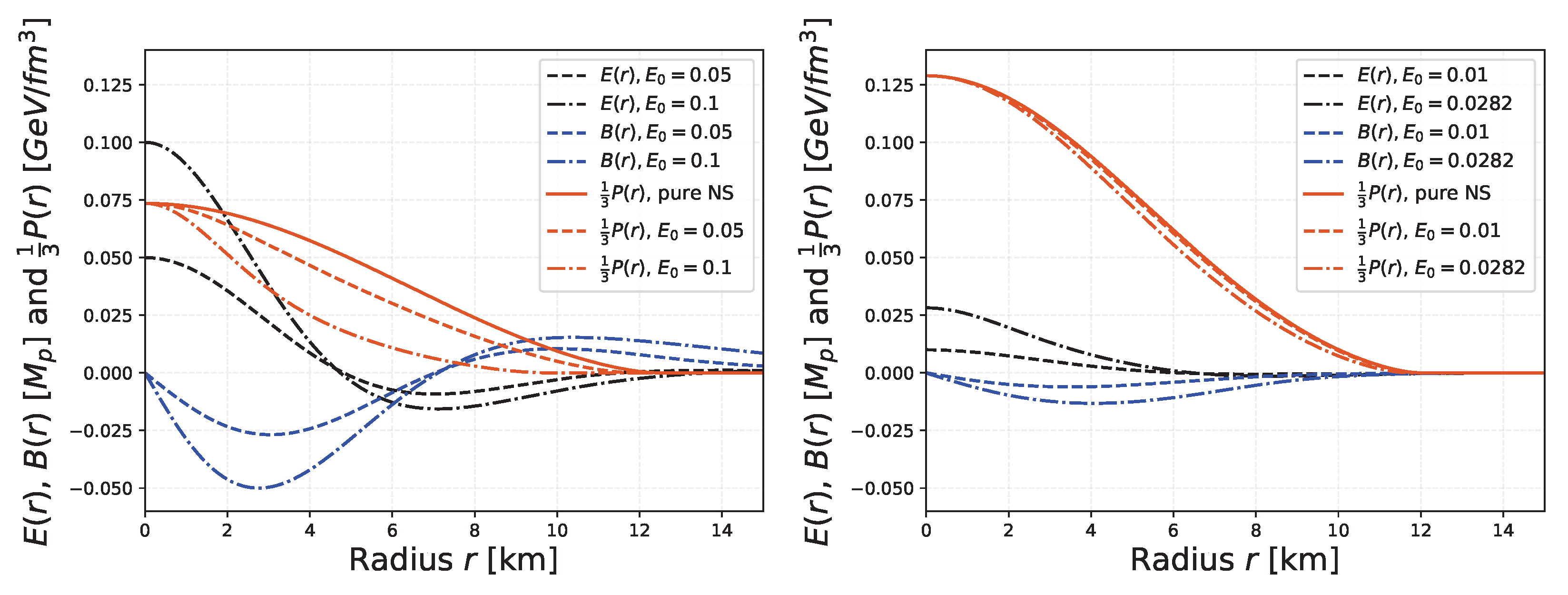
In Figure 1, we show radial profiles of the pressure (orange) and the vector field components (black), (blue) of the zeroth mode of different FPSs with potential Equation (22). In the left panel, we take a boson mass of eV and an interaction strength of . The FPSs have varying central vector field amplitudes and central densities of . Here, we take g/cm3 to be the nuclear saturation density, with being the neutron mass and fm−3 the average nuclear number density. The radial profile of a pure NS is shown with the orange continuous line and has no corresponding vector field (because it would be zero everywhere). The presence of the DM can be seen to compactify the NS component with increasing central field amplitude . The field forms a DM core configuration.
In the right panel of Figure 1, all the parameters are left equal except for the vector boson mass, which is set to eV. Due to the low DM mass, the correlation length increases, which increases the size of the vector field component and forms a DM cloud configuration. Since the amount of energy density of the vector field is distributed inside and outside the NS component, the effect on the radius is small. At around km, a kink can be seen in the radial profile of the field component . This point coincides with the point where the fermionic radius of the FBS is located. This illustrates the gravitational backreaction between the vector field and the NS component of the FBS.
In Figure 2, we show radial profiles of the pressure (orange) and the vector field components (black), (blue) of an FPS. In the left panel, we show an FPS in the first mode, which can be identified by the fact that the component crosses the x-axis twice and crosses it once. The boson mass is eV and . This time, the central density is taken to be , and the central vector field amplitudes vary.
The right panel of Figure 2 shows an FPS in the zeroth mode with a vector boson mass of eV and a self-interaction strength of . The maximal amplitude is roughly due to the analytical bound on ; see Equation (24). The limited field amplitude strongly limits the possible effect on the fermionic component and thus on the fermionic radius, especially in the limit of large . It may therefore be difficult to detect strongly self-interacting vector DM within an NS if one only considers measurements of the fermionic radius. It is also conceivable that the maximum amplitude implies a maximum amount of possible accretion of vector DM, which could be used to set bounds on the DM self-interaction strength. We leave the analysis of this aspect for a future work.
3.2. Stable Solutions
We compute a grid of FPSs with different central densities and central vector field amplitudes . Using the array of solutions, we compute the stability curve using stability criterion Equation (26). The stable solutions can then be filtered and analyzed further.
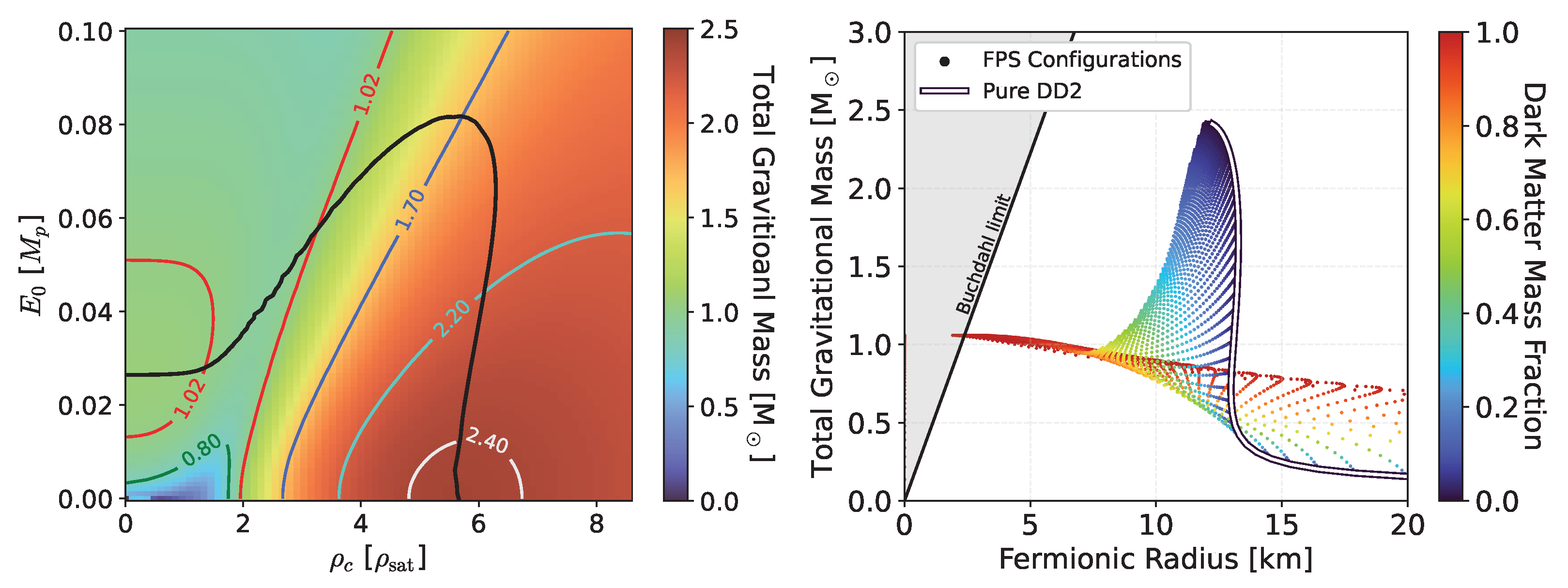
This can be seen in the left panel of Figure 3, where we compute FPSs with quartic self-interaction potential Equation (22) with eV and . We additionally compute the stability curve using stability criterion Equation (26). The stability curve defines the boundary between stable and unstable configurations under linear radial perturbations. The shape of the stability curve for FPSs is qualitatively very similar to the case of scalar FBSs (compare to [15]). For pure neutron stars and Proca stars, respectively, the curve converges on the - and -axes at the point where the non-mixed configurations have their maximum gravitational masses. We take only the FPSs inside the stability region, enclosed by the stability curve, and plot them in a mass–radius (MR) diagram. This leads to the graph in the right panel of Figure 3.
We see that stable FPS configurations form an MR region instead of an MR curve (which would be the case for single-fluid systems). The stable configurations form core or cloud solutions, depending on their DM fraction . A DM core is present if the bosonic component is geometrically smaller than the fermionic component (i.e., when ). The opposite is true for cloud configurations. The FPSs with high DM fractions have masses of roughly . This is higher than for scalar FBSs with equal boson mass m (compare to [15]). This can be explained through the different scaling relations for pure Proca stars and boson stars.
Another point where FPSs differ from FBSs is the existence of maximal amplitude Equation (24) for the vector field. When increasing the self-interaction strength , the maximal possible vector field amplitude shrinks. This affects the shape of the stability curve.
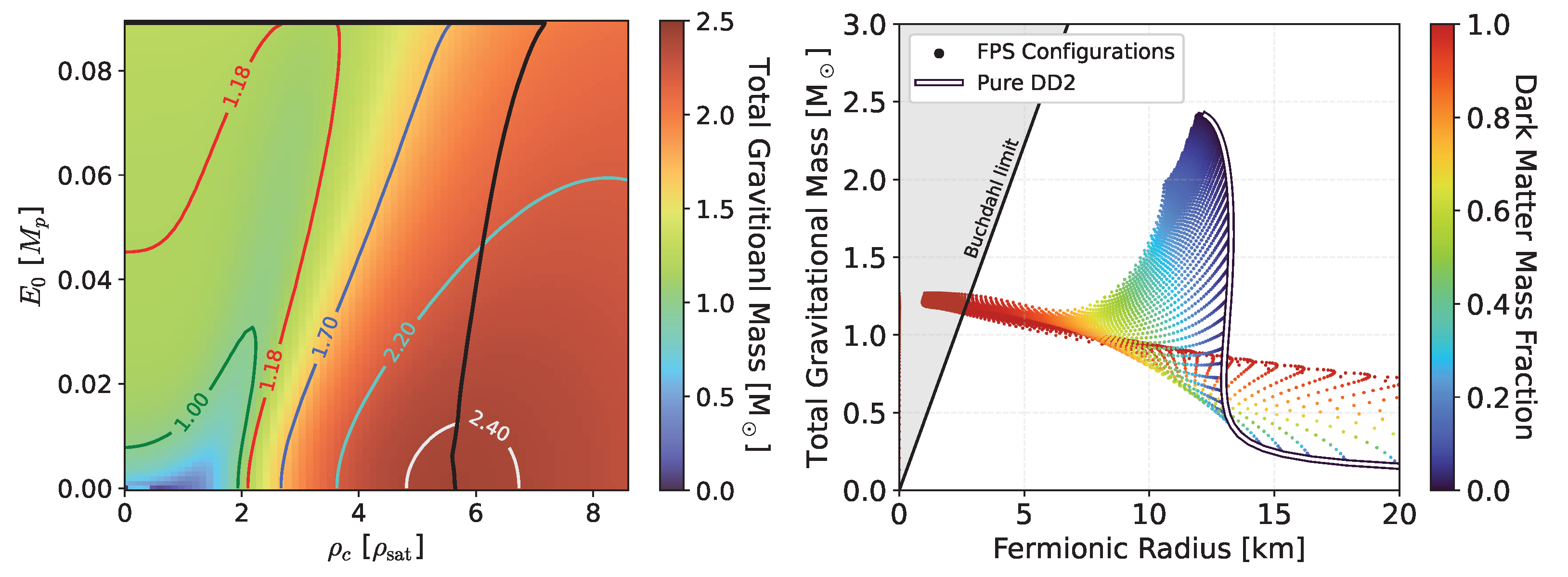
In Figure 4 (left panel), we show such a case where the self-interaction strength is . The stability curve does not reach the -axis anymore but instead rises vertically from the pure NS configurations until it reaches the FPSs with maximal central vector field amplitude . We have manually extended the stability curve so that it proceeds horizontally until it reaches the -axis. It is noteworthy that this behavior starts at surprisingly small self-interaction strengths and persists up to higher .
In principle, a third behavior of the stability curve of FPSs is also conceivable. For some specific , it should be possible that the stability curve does not admit one continuous shape like in Figure 3 and Figure 4 but that the stability curve is cut into two parts, namely one part that starts at the -axis and then rises to reach the edge where is located and another part that starts at the -axis and then rises roughly vertically until it too reaches the analytical bound for the vector field amplitude (think of a horizontal line cutting through the stability curve in Figure 3 at, e.g., ). During our testing, we did not find any case where the stability curve follows this behavior. However, there is also no reason that we are aware of as to why such a behavior of the stability curve should be forbidden. This is why we presume that such a case might exist.
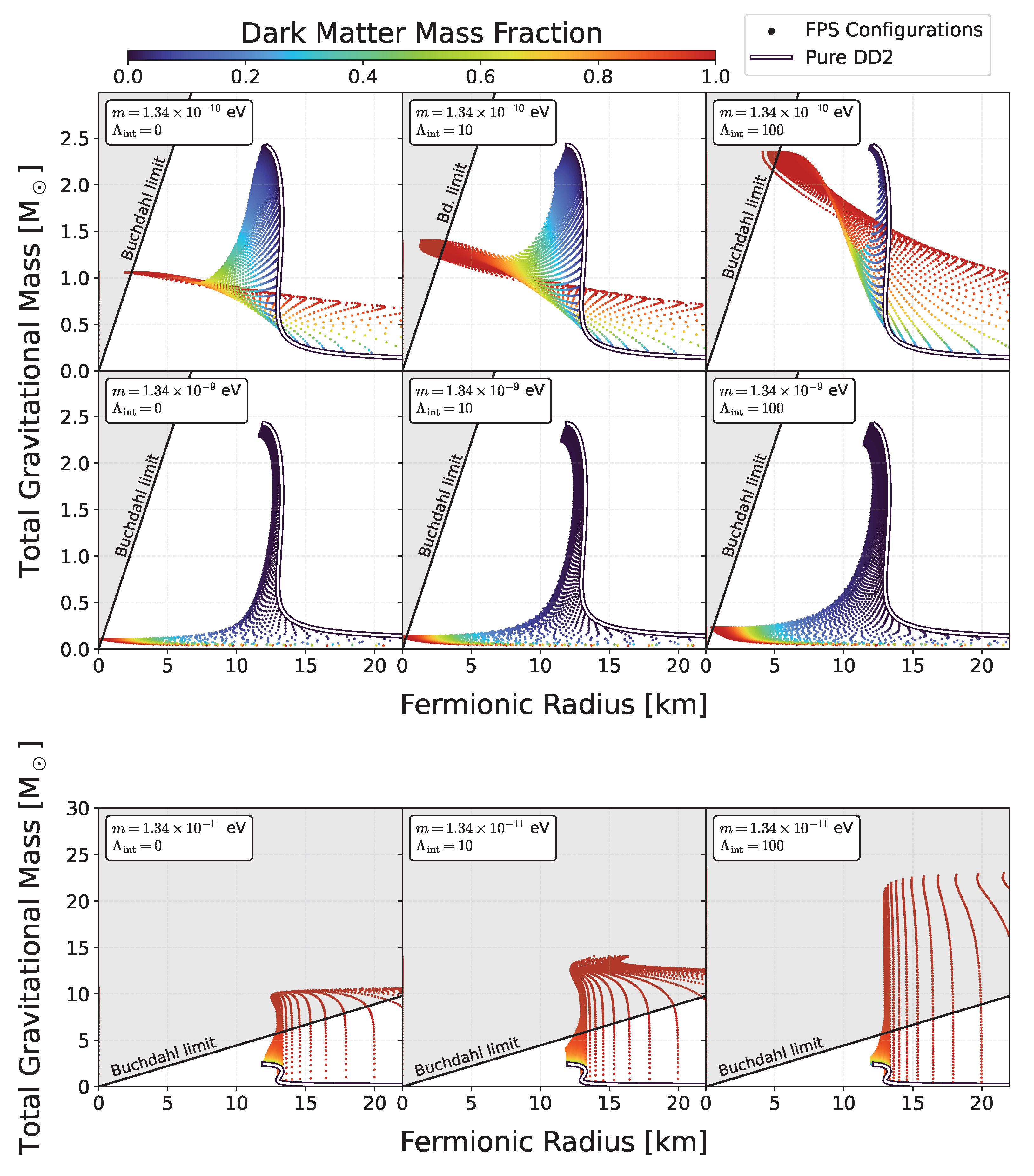
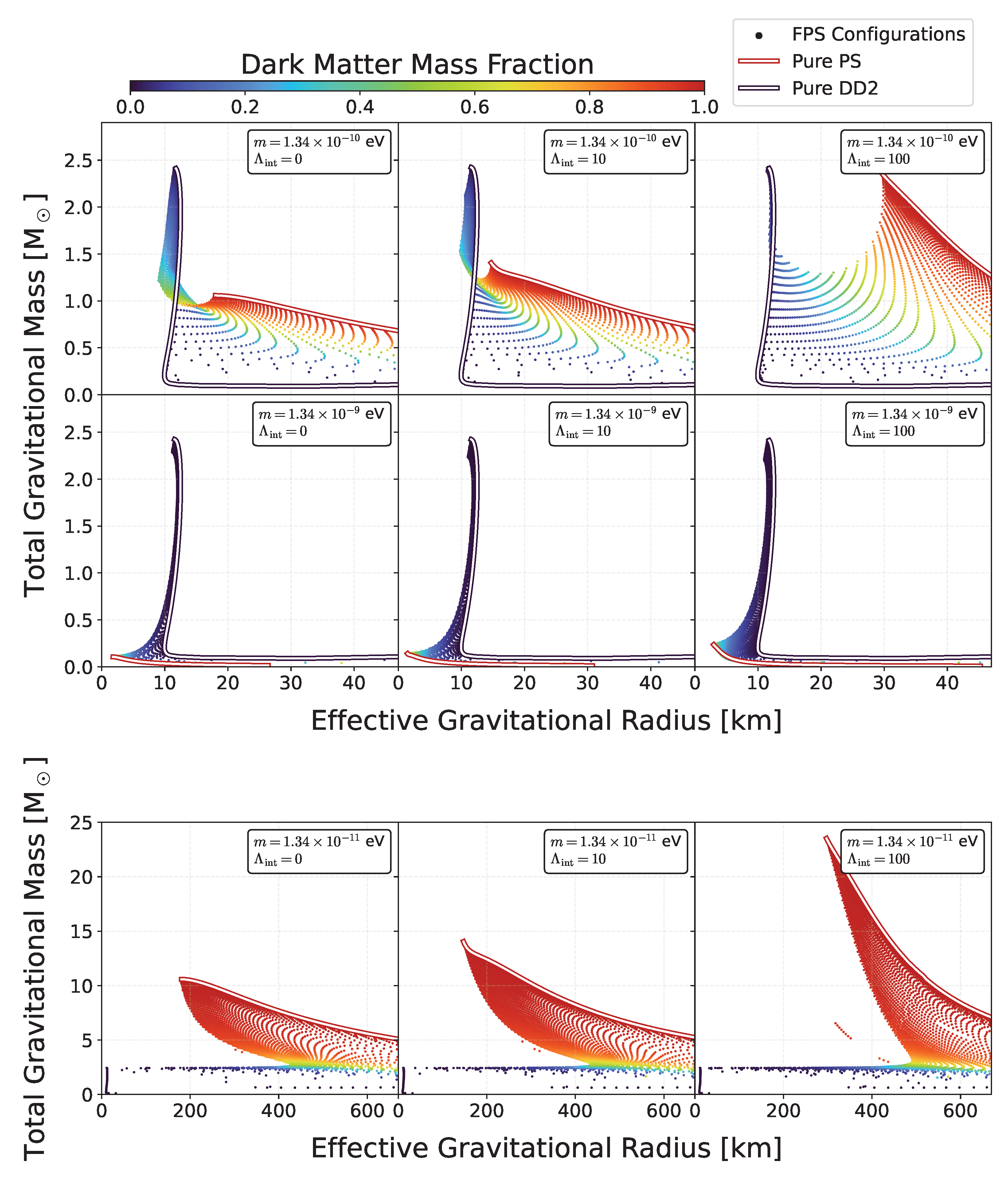
We compute various FPSs with different values of vector boson masses eV and self-interaction strengths . We chose the same parameter values as in [15] to allow for easy comparability. In Figure 5, we show the mass and fermionic radii of all stable FPS configurations in an MR diagram. In Figure 6, we show the mass plotted against the effective gravitational radius . It is defined as the radius where of the total restmass is contained. The stable solutions have been obtained using stability criterion Equation (26). Note the different axis scaling in the figures. It was chosen such that the relevant trends and features of the solutions can be seen well.
We hereafter discuss some general trends and compare the results to the one obtained for scalar FBSs. The following analysis should thus be explicitly compared to Figure 2 and 3 in [15].
We find that many of the general conclusions regarding FBSs can also be applied to FPSs. FPSs with small DM fractions are dominated by the fermionic component, leading to only small changes in the fermionic radius. In the case of DM-dominated FPSs, the solutions behave similarly to pure Proca stars. This leads to higher masses as compared to FBSs, where the total gravitational mass of pure boson stars will be roughly half that of a Proca star with the same boson mass, as can be seen well for the cases where eV. FPSs can thus reach higher total gravitational masses as compared to FBSs with the same DM mass and self-interaction strength.
For eV, the bosonic component is concentrated inside the fermionic one and forms a DM core. Even small amounts of DM can have a significant impact on the fermionic radius since the whole vector field is concentrated entirely inside the NS component. More massive DM particles can thus have larger effects on the fermionic radius compared to low-mass DM at similar DM fractions. This is due to the cloud-like structure of low-mass DM. For small DM masses, the majority of the DM will be concentrated outside the NS part—due to its larger correlation length—and will thus have smaller effects on the fermionic radius. The smaller the mass and the larger the self-interaction strength, the more likely the formation of a DM cloud is. The opposite is true for DM core solutions. FPSs tend to produce configurations with larger total masses compared to scalar FBSs. Their halos also extend to larger radii, as can be seen from the gravitational radius in Figure 6.
In general, the gravitational radius of FPSs is larger in size as compared to scalar FBSs (compare to Figure 3 in [15]). The larger gravitational radius suggests that FPS have larger tidal deformabilities compared to their scalar field counterparts (FBS) with equal m and . This is because objects with larger radii are generally favored to tidally disrupt. This could favor higher vector boson masses compared to the corresponding scalar boson mass in the case of FBSs. A future quantitative analysis of the tidal deformability in FPSs is needed to definitively verify this hypothesis.
When considering the gravitational radius of FPSs with small boson masses of eV (bottom row of Figure 6), the transition between DM-dominated and NS-dominated configurations appears more abrupt than in the FBS case (compare to Figure 3 in [15]). For example, when starting with a system with a DM fraction of roughly or , increasing the DM fraction by small amounts can massively impact the total mass and gravitational radius of the combined system.
Finally, note the outlier points in Figure 6 for eV and at roughly km. These are likely to be numerical artifacts and should thus not be regarded as physical. This is to be expected since, for small DM masses and large self-interactions, the numerical solution becomes increasingly difficult. This problem could be avoided by using smaller step sizes and higher numerical precision. However, this would also lead to longer runtimes of the code.
3.3. Comparison with Scalar FBS
We show MR relations of FPSs and scalar FBSs with fixed DM fractions .
In the left panel of Figure 7, we show different FPSs with constant DM fractions. The DD2 EOS [96] was used for the NS component. For the vector boson, we chose masses of eV and no self-interactions. This figure should be explicitly compared to Figure 5 (left panel) in [15] as the same masses and DM fractions were chosen. The MR curve of a pure NS with the DD2 EOS (black line) is shown as a reference. Depending on the boson mass, FPSs can have increased or decreased maximum total gravitational mass when there is vector DM present. FPSs tend to produce configurations with larger gravitational masses compared to FBSs with equal parameters (mass, self-interaction, and DM fraction). This is not surprising when considering the scaling relations of pure boson stars and Proca stars, respectively. The gravitational mass scales like /m for pure boson stars and like /m for pure Proca stars, where m is the mass of the scalar/vector boson, respectively. The presence of light bosonic DM can help to increase the total gravitational mass of an NS. This can create EOSs that do not fulfill the observational constraints for the maximum NS mass viable again. Vector DM has a larger effect on the gravitational mass than scalar DM, and thus smaller amounts of vector DM are needed to produce an equal increase in the total gravitational mass.
In the right panel of Figure 7, we show different FPSs (orange and green lines) and FBSs (blue lines) for different boson masses, no self-interactions, and constant DM fractions . We used the DD2 EOS [96] for the NS component. The parameters were chosen in a way to illustrate the degeneracies that can arise from different DM models or EOSs for the NS component. For example, FPSs and FBSs with boson masses of eV (dashed lines) produce virtually indistinguishable mass–radius relations when the FPSs and the FBSs have a DM fraction of and respectively. A similar behavior can be seen for the cases where the boson mass is eV (dot-dashed lines). Here, FBSs with DM fraction produce similar MR curves to FPSs with DM fraction. In addition, the resulting MR curves are comparable to the curve corresponding to a pure NS with the KDE0v1 EOS [100]. They also match the curve corresponding to an FPS with DM fraction and a vector boson mass of eV (green line).
In conclusion, FPSs can produce degenerate results in the MR plane with both FBSs and pure NS given that different DM fractions and EOSs are allowed. Additional observables, such as tidal deformability, are needed to break the degeneracy. However, it seems difficult to prevent degenerate solutions from existing in general since FPSs themselves can be degenerate with other FPS solutions that have different boson masses and DM fractions.
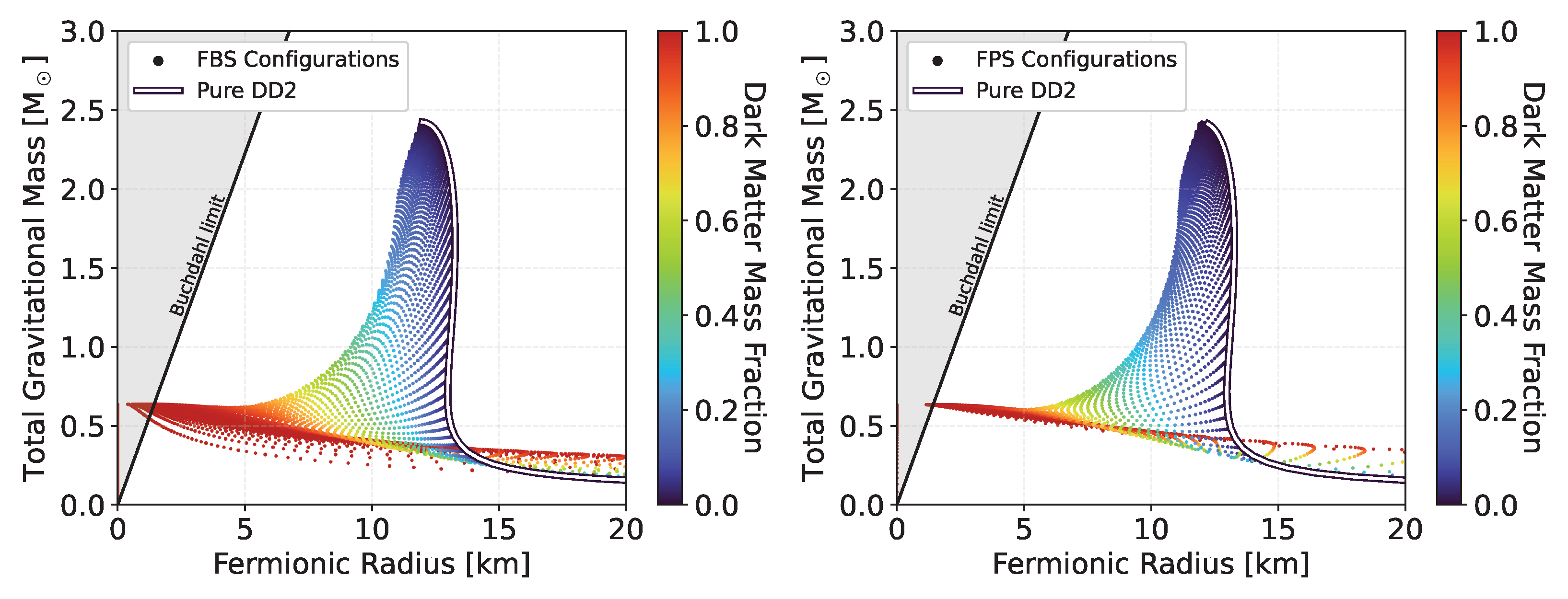
We further explore the degeneracy between FPS and FBS solutions. In Figure 8, we show the stable FBS and FPS solutions in an MR diagram. We used the scaling relations of the maximum mass for pure boson stars (/m) and pure Proca stars (/m) to match the boson masses in a way that both FPSs and FBSs will have the same gravitational mass in the pure boson star/Proca star limit. To guarantee matching solutions in this limit, we chose a scalar boson mass of eV and we chose a mass of times the mass of the scalar boson—i.e., eV—for the vector boson. We find a high degree of similarity between the MR region of FBSs and FPSs with the scaled masses. This makes both solutions almost indistinguishable. The small differences present between the left and right panel of Figure 8 can be attributed to slightly different grid spacing used for the initial conditions , (and , ). This can be seen in the MR regions at small total gravitational masses and also at radii km. The color shading further reveals a different distribution of DM fractions for a given and , even though the difference is small.
We expect a similar behavior to hold when considering different scalar and vector boson masses (with zero self-interaction) given that they differ by the same factor of ≈1.671. This adds further confidence to the observation that FBSs and FPSs might be difficult to distinguish since a given solution might be another system but with different boson mass (or DM fraction).
Similar scaling relations also exist for boson stars and Proca stars in the limit of large self-interactions . A similar procedure might therefore be possible when also matching the self-interaction strength appropriately. An independent measurement of the DM particle mass would break this degeneracy to a certain degree. However, it would also be necessary to constrain the self-interaction strength and the DM fraction through other means, for example, using correlations of the DM abundance in the galactic disk (see [101,102]) or using the bound on the maximal vector field amplitude.
The scaling behavior between (fermion) boson stars and (fermion) Proca stars also suggests another application. If it persists for large non-zero self-interactions, it might be possible to also use the effective bosonic EOS derived by Colpi et al. [103] to model (fermion) Proca stars. Since the EOS by Colpi et al. was originally derived for a scalar field, one would then have to scale the boson mass by a factor of and the self-interaction by an appropriate amount. The necessary scaling for the self-interaction will be dictated by the scaling relations for pure boson stars (/m [103]) and Proca stars (/m [84]) at large self-interaction strengths. We note, however, that great care is needed since Proca stars technically do not exist in the limit of large self-interactions (see the analytical bound on vector field amplitude Equation (24)). We plan to study this aspect in the future.
3.4. Higher Modes and Different EOSs
We broaden our analysis to FPSs with different EOSs for the fermionic component and to FPSs where the bosonic component exists in a higher mode. Higher modes are usually assumed to be unstable, but, as numerical simulations of scalar boson stars have shown [37,104], higher modes might be dynamically stable when gravitationally interacting in a multi-component system. We therefore start by considering FPSs in the first and second mode in Figure 9.
In the left panel of Figure 9, we show the total gravitational mass and the fermionic radius of stable FPS configurations, where the bosonic component is in the first mode (as opposed to the ground mode, which is the zeroth mode). The vector boson mass is eV, and the self-interaction is set to zero. We first note the fact that stable solutions under linear radial perturbations, according to stability criterion Equation (26), exist at all. This is a non-trivial statement as higher modes of Proca stars (and also of scalar boson stars) are usually believed to be unstable. Note, however, that stability criterion Equation (26) is merely a necessary condition for stability and that there could be additional conditions that must be fulfilled for a solution to be stable in higher modes. Also, our stability analysis does not consider the dynamical stability of the higher modes. They might thus be unstable in non-static scenarios. It is, however, possible that the higher modes of the bosonic part might be stabilized through the gravitational interaction with the fermionic part of the FPS. In general, solutions in higher modes need energy to be supported or excited. Otherwise, they would decay to the ground mode. The authors of [104] explicitly studied the stability of higher modes for scalar boson stars with multiple scalar fields. They investigated cases where one field is in the ground mode and another is in the excited state. They found that the excited mode is stable if the charge of the conserved Noether current (which can also be interpreted as the particle number or the total restmass; see Equation (11)) of the ground mode is larger than the Noether charge of the excited mode: . If this logic also holds for mixed systems of fermions and bosons, this would imply an additional stability condition that the fermion number must be larger than the boson number of the FPS in the excited mode. We further refer to chapter 3.7 in [30] for a more detailed review.
The FPSs in the first mode exhibit higher gravitational masses in the configurations dominated by the bosonic component, compared to FPSs in the zeroth mode (compare to Figure 3). The numerical value of the frequency in the higher mode is also larger than the frequency in lower modes. This behavior is consistent with earlier works, which studied pure Proca stars analytically [84] and numerically [79]. They also observed that higher frequencies lead to larger total gravitational mass. The left panel of Figure 9 shows a number of outlier points at around 11 km and . These are likely numerical artifacts due to the increased difficulty in finding accurate numerical solutions for higher modes.
The right panel of Figure 9 shows stable FPS configurations in the second mode. The vector boson mass is eV and the self-interaction is set to zero. Here also, the existence of stable solutions is to be acknowledged. In the limit of high DM fractions, the FPSs converge to the solution of pure Proca stars and reach total gravitational masses of roughly times that of Proca stars in the zeroth mode (compare to Figure 3). In comparison to the case in the first mode (left panel of Figure 9), the quality of the overall solution can be seen to deteriorate further. We believe the outlier points at roughly <13 km and to be non-physical numerical artifacts. The outlier points coincide with the solutions in the zeroth mode. This suggests that our solver did not find the second mode in these cases and converged on the zeroth mode instead. Solutions of FPSs in even higher modes should therefore be considered with great care. The difficulty in obtaining accurate numerical solutions is likely to increase further for higher modes. The quality of the solution is, however, sufficient to gain a qualitative understanding of FPSs in higher modes. In conclusion, higher modes are stable under linear radial perturbations and increase the total gravitational mass of FPSs by substantial amounts.
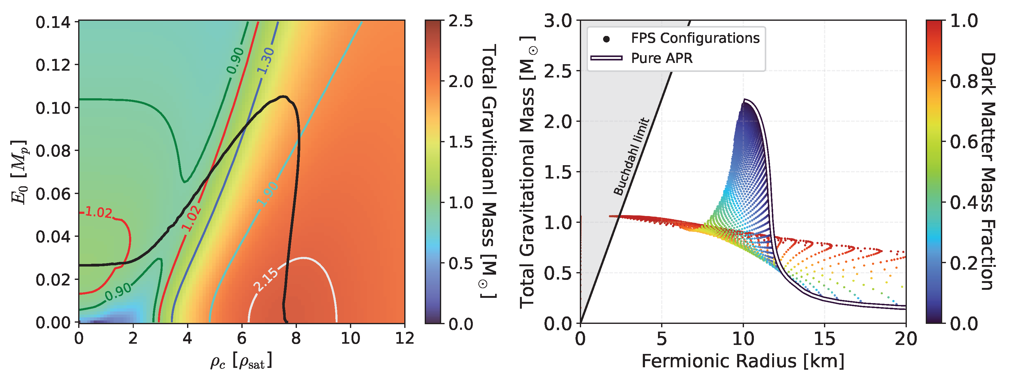
We investigate the effect that different EOSs have on FPSs. In Figure 10, we use the APR EOS [105] for the fermionic part. We chose a vector boson mass of eV with no self-interaction for the bosonic part. In the left panel, we notice that the shape of the stability curve (black curve) is affected by the choice in the EOS. On the -axis, it converges to a value of around . This is higher than the corresponding value of when the DD2 EOS is used (compare to Figure 3) because the APR EOS is softer than the DD2 EOS. This means that the nuclear matter is easier to compress and higher central densities can be supported by the EOS. The easier compressibility also shows itself through smaller NS radii (see the right panel). In the limit of pure Proca stars, the stability curve converges to the same value as it does when the DD2 EOS is used (compare to Figure 3). The MR region shows a similar qualitative behavior as in the DD2 case. The high DM fraction limit in particular shows a convergence to the solution to pure Proca stars. The APR EOS also allows higher central amplitudes of the vector field , compared to the DD2 EOS with equal boson mass and self-interaction strength.
Figure 11 shows different FPS configurations where the FSG EOS [96] was used for the fermionic part. For the bosonic part, we used a boson mass of eV and no self-interaction. The FSG EOS is a soft EOS and thus reaches higher central densities for pure NSs. It is excluded by current observational constraints (see Figure 7) as it cannot produce pure NSs with masses of [8]. However, adding DM to the pure NSs can significantly increase the maximum gravitational mass of the combined system. The FSG EOS is then able to reach the observational bound on the maximum NS mass in the presence of DM. In fact, the MR curve of the pure DD2 EOS is entirely contained within the stability region of the FPSs with the FSG EOS. This again raises the point that some FPS solutions are degenerate with some NS solutions (see Figure 8), when allowing for different DM fractions and DM masses. Another factor complicating the identification of the EOS vs. the DM effects is that the presence of dark matter might change the fermionic radius produced by a given EOS. For example, [92] found that the presence of self-interacting and repulsive fermionic dark matter can lead to nearly indistinguishable fermionic radii for different EOS. To figure out whether and which types of mixed DM–NS systems might exist, it will be crucial to perform sophisticated parameter searches of the system and obtain more measurements to constrain the DM and NS properties in future studies.
4. Conclusions
In this work, we studied the impact that bosonic dark matter (DM) has on the mass and radius of neutron stars (NSs). DM was modeled as a massive self-interacting complex vector field. DM was further assumed to only interact gravitationally with the fermionic neutron star matter. We derived the equations of motion describing static spherically symmetric fermion Proca stars (FPSs) and computed their properties numerically. We also found a scaling relation between the frequency, vector field, and metric components, and we derived an analytical upper bound on the vector field amplitude.
We showed that the presence of the vector field can lead to core-like and to cloud-like solutions. Core-like solutions can increase the compactness of the NS component. For some configurations, observing only the fermionic radius and the total gravitational mass would appear to violate the Buchdahl limit. We found core-like solutions for vector boson masses of eV and small self-interactions m2. Cloud-like solutions appeared when eV and is large. For some small boson masses eV, the presence of DM can significantly increase the total gravitational mass while leaving the fermionic radius approximately constant.
We computed radial profiles of FPSs and found that the existence of a maximum possible vector field amplitude limits the effect of DM on the NS when the self-interaction is large. The maximum amplitude implies a maximum possible amount of vector boson DM accretion and could thus be used to set bounds on the DM properties.
We also compared FPSs to FBSs with a scalar field. We used the same parameters as in [15] to simplify the comparison. For stable FPS configurations, we found that many of the general qualitative trends that apply to FBSs also apply to FPSs. However, vector DM leads to higher FPS masses and larger gravitational radii for equal m and . This could also imply a larger tidal deformability in FPSs compared to FBSs. Also, a measurement of the gravitational radius would favor larger vector boson masses compared to scalar boson masses.
For FPS configurations of constant DM fraction, we found that the effect of vector DM on the NS properties (total gravitational mass and fermionic radius) is larger compared to FBSs with equal DM fraction, mass m, and self-interaction strength . One therefore needs a larger amount of scalar DM to cause the same effect as vector DM. For different boson masses and DM fractions, we found that FPSs and FBSs can both be degenerate with each other and also be degenerate with pure NS with a different EOS.
We found an especially high degree of similarity between FBS solutions with no self-interaction and a boson mass of eV with FPS solutions where the vector boson mass is larger by a factor of . We expect the similarity in the behavior to also hold for different boson masses (and also for non-zero self-interactions), as long as the vector boson mass is scaled accordingly by the right factor.
These similarities also hint towards a possibility to also use the effective EOS by Colpi et al. [103] for (fermion) Proca stars. We note, however, that great care is needed since Proca stars do not exist in the limit of large self-interactions (see the analytical bound on vector field amplitude Equation (24)). The similarities between FBSs and FPSs might also be useful for numerical applications. Scalar (fermion) boson stars are easier to implement and numerically cheaper to solve than FPSs. One could then simply solve the equations for scalar (fermion) boson stars with a re-scaled mass (and self-interaction parameter ) to compute the properties (, ) of (fermion) Proca stars.
The prevalence of degenerate solutions highlights the importance of measuring additional observables, such as the tidal deformability, to break the degeneracies.
We confirmed the existence of higher modes that are stable under first-order radial perturbations. We found that higher modes lead to higher total gravitational masses of the mixed FPS systems. Using FPSs with different EOSs for the fermionic part, we explicitly confirmed that, for certain DM masses, previously excluded EOSs are able to fulfill observational bounds if DM is present. Mixed systems of bosonic DM and NS matter can therefore be consistent with all the current observational constraints if suitable boson masses and self-interaction strengths are chosen.
Author Contributions
Conceptualization, C.J. and L.S.; methodology, C.J.; software, C.J.; validation, C.J.; formal analysis, C.J.; investigation, C.J.; resources, L.S.; data curation, C.J.; writing—original draft preparation, C.J.; writing—review and editing, C.J. and L.S.; visualization, C.J.; supervision, L.S.; project administration, C.J. and L.S.; funding acquisition, L.S. All authors have read and agreed to the published version of the manuscript.
Funding
This research was funded by the Deutsche Forschungsgemeinschaft (DFG, German Research Foundation) through the CRC-TR 211 ‘Strong-interaction matter under extreme conditions’—project number 315477589-TRR 211.
Data Availability Statement
The code used to produce all results in this work, including scripts to create the figures shown in this work, can be found in the GitHub repository FBS-Solver (see [88]). The code used to compute the configurations with the vector field can be found on the repository branch “vector-fbs”. All data is openly available in this repository branch. Further inquiries can be directed to the corresponding author.
Acknowledgments
The authors acknowledge support by the Deutsche Forschungsgemeinschaft (DFG, German Research Foundation) through the CRC-TR 211 ‘Strong-interaction matter under extreme conditions’—project number 315477589-TRR 211. C.J. acknowledges support by the Hermann-Wilkomm-Stiftung 2023.
Conflicts of Interest
The authors declare no conflict of interest.
Appendix A. Units
In this work, we use units in which the gravitational constant, the speed of light, and the solar mass are set to . As a direct consequence, distances are measured in units of , which corresponds to half the Schwarzschild radius of the Sun (also called the gravitational radius of the Sun). The Planck mass is . Since , it follows that .
Boson stars (with a scalar field) are described using the Klein–Gordon equation, which in SI units and flat spacetime reads . The term is the inverse of the reduced Compton wavelength , which sets the typical length scale for the system even in the self-gravitating case. We assume that the typical length scale of the boson is similar to the gravitational radius , which in the case of mass scales of ∼1 is approximately km. With , this therefore leads to a mass scale of the bosonic particle of eV. Previous works such as, e.g., [15,33], thus specify the mass of the scalar particle in these units. A mass of in our numerical code [88] then also corresponds to eV. This choice in the boson mass then automatically leads to boson stars with masses in the range of . The same reasoning can also be applied to the case where the boson is a vector boson. This is valid since all components of a vector field also fulfill the Klein–Gordon equations individually.
References
Ade, P.A.R.; Aghanim, N.; Arnaud, M.; Ashdown, M.; Aumont, J.; Baccigalupi, C.; Banday, A.J.; Barreiro, R.B.; Bartlett, J.G.; Bartolo, N.; et al. Planck 2015 results. XIII. Cosmological parameters. Astron. Astrophys.2016, 594, A13. [Google Scholar] [CrossRef]
Bertone, G.; Hooper, D. History of dark matter. Rev. Mod. Phys.2018, 90, 045002. [Google Scholar] [CrossRef]
White, S.D.M.; Frenk, C.S.; Davis, M. Clustering in a Neutrino Dominated Universe. Astrophys. J. Lett.1983, 274, L1–L5. [Google Scholar] [CrossRef]
Blumenthal, G.R.; Faber, S.M.; Primack, J.R.; Rees, M.J. Formation of Galaxies and Large Scale Structure with Cold Dark Matter. Nature1984, 311, 517–525. [Google Scholar] [CrossRef]
Davis, M.; Efstathiou, G.; Frenk, C.S.; White, S.D.M. The Evolution of Large Scale Structure in a Universe Dominated by Cold Dark Matter. Astrophys. J.1985, 292, 371–394. [Google Scholar] [CrossRef]
Tolman, R.C. Static solutions of Einstein’s field equations for spheres of fluid. Phys. Rev.1939, 55, 364–373. [Google Scholar] [CrossRef]
Romani, R.W.; Kandel, D.; Filippenko, A.V.; Brink, T.G.; Zheng, W. PSR J0952−0607: The Fastest and Heaviest Known Galactic Neutron Star. Astrophys. J. Lett.2022, 934, L17. [Google Scholar] [CrossRef]
Abbott, R.; Abbott, T.D.; Abraham, S.; Acernese, F.; Ackley, K.; Adams, C.; Adhikari1, R.X.; Adya, V.B.; Affeldt, C.; Agathos, M.; et al. GW190814: Gravitational Waves from the Coalescence of a 23 Solar Mass Black Hole with a 2.6 Solar Mass Compact Object. Astrophys. J. Lett.2020, 896, L44. [Google Scholar] [CrossRef]
Most, E.R.; Papenfort, L.J.; Weih, L.R.; Rezzolla, L. A lower bound on the maximum mass if the secondary in GW190814 was once a rapidly spinning neutron star. Mon. Not. Roy. Astron. Soc.2020, 499, L82–L86. [Google Scholar] [CrossRef]
Riley, T.E.; Watts, A.L.; Bogdanov, S.; Ray, P.S.; Ludlam, R.M.; Guillot, S.; Arzoumanian, Z.; Baker, C.L.; Bilous1, A.V.; Chakrabarty, D.; et al. A NICER View of PSR J0030+0451: Millisecond Pulsar Parameter Estimation. Astrophys. J. Lett.2019, 887, L21. [Google Scholar] [CrossRef]
Riley, T.E.; Watts, A.L.; Ray, P.S.; Bogdanov, S.; Guillot, S.; Morsink, S.M.; Bilous, A.V.; Arzoumanian, Z.; Choudhury, D.; Deneva, J.S.; et al. A NICER View of the Massive Pulsar PSR J0740+6620 Informed by Radio Timing and XMM-Newton Spectroscopy. Astrophys. J. Lett.2021, 918, L27. [Google Scholar] [CrossRef]
Abbott, B.P.; Abbott, R.; Abbott, T.D.; Acernese, F.; Ackley, K.; Adams, C.; Adams, T.; Addesso, P.; Adhikari, R.X.; Adya, V.B.; et al. GW170817: Measurements of neutron star radii and equation of state. Phys. Rev. Lett.2018, 121, 161101. [Google Scholar] [CrossRef] [PubMed]
Abbott, B.P.; Abbott, R.; Abbott, T.D.; Acernese, F.; Ackley, K.; Adams, C.; Adams, T.; Addesso, P.; Adhikari, R.X.; Adya, V.B.; et al. Properties of the binary neutron star merger GW170817. Phys. Rev.2019, X9, 011001. [Google Scholar] [CrossRef]
Diedrichs, R.F.; Becker, N.; Jockel, C.; Christian, J.E.; Sagunski, L.; Schaffner-Bielich, J. Tidal deformability of fermion-boson stars: Neutron stars admixed with ultralight dark matter. Phys. Rev. D2023, 108, 064009. [Google Scholar] [CrossRef]
Goldman, I.; Nussinov, S. Weakly Interacting Massive Particles and Neutron Stars. Phys. Rev. D1989, 40, 3221–3230. [Google Scholar] [CrossRef] [PubMed]
Rutherford, N.; Raaijmakers, G.; Prescod-Weinstein, C.; Watts, A. Constraining bosonic asymmetric dark matter with neutron star mass-radius measurements. Phys. Rev. D2023, 107, 103051. [Google Scholar] [CrossRef]
Bertone, G.; Fairbairn, M. Compact Stars as Dark Matter Probes. Phys. Rev. D2008, 77, 043515. [Google Scholar] [CrossRef]
Ellis, J.; Hütsi, G.; Kannike, K.; Marzola, L.; Raidal, M.; Vaskonen, V. Dark Matter Effects On Neutron Star Properties. Phys. Rev. D2018, 97, 123007. [Google Scholar] [CrossRef]
Shirke, S.; Ghosh, S.; Chatterjee, D.; Sagunski, L.; Schaffner-Bielich, J. R-modes as a New Probe of Dark Matter in Neutron Stars. arXiv2023, arXiv:2305.05664v2. [Google Scholar] [CrossRef]
Karkevandi, D.R.; Shakeri, S.; Sagun, V.; Ivanytskyi, O. Bosonic dark matter in neutron stars and its effect on gravitational wave signal. Phys. Rev. D2022, 105, 023001. [Google Scholar] [CrossRef]
Khlopov, M.; Malomed, B.A.; Zeldovich, I.B. Gravitational instability of scalar fields and formation of primordial black holes. Mon. Not. Roy. Astron. Soc.1985, 215, 575–589. [Google Scholar] [CrossRef]
Biswas, S.; Gabrielli, E.; Mele, B. Dark Photon Searches via Higgs Boson Production at the LHC and Beyond. Symmetry2022, 14, 1522. [Google Scholar] [CrossRef]
An, H.; Ge, S.; Liu, J. Solar Radio Emissions and Ultralight Dark Matter. Universe2023, 9, 142. [Google Scholar] [CrossRef]
Foschi, A.; Abuter, R.; Dayem, K.; Aimar, N.; Seoane, P.A.; Amorim, A.; Berger, J.P.; Bonnet, H.; Bourdarot, G.; Brandner, W.; et al. Using the motion of S2 to constrain vector clouds around SgrA. arXiv2023, arXiv:2312.02653. [Google Scholar]
Kouvaris, C.; Tinyakov, P. Can Neutron stars constrain Dark Matter? Phys. Rev. D2010, 82, 063531. [Google Scholar] [CrossRef]
Liebling, S.L.; Palenzuela, C. Dynamical boson stars. Living Rev. Rel.2023, 26, 1. [Google Scholar] [CrossRef]
Zurek, K.M. Asymmetric Dark Matter: Theories, Signatures, and Constraints. Phys. Rept.2014, 537, 91–121. [Google Scholar] [CrossRef]
Kouvaris, C. The Dark Side of Neutron Stars. Adv. High Energy Phys.2013, 2013, 856196. [Google Scholar] [CrossRef]
Di Giovanni, F.; Sanchis-Gual, N.; Cerdá-Durán, P.; Font, J.A. Can fermion-boson stars reconcile multimessenger observations of compact stars? Phys. Rev. D2022, 105, 063005. [Google Scholar] [CrossRef]
Nelson, A.; Reddy, S.; Zhou, D. Dark halos around neutron stars and gravitational waves. J. Cosmol. Astropart. Phys.2019, 7, 12. [Google Scholar] [CrossRef]
Baryakhtar, M.; Caputo, R.; Croon, D.; Perez, K.; Berti, E.; Bramante, J.; Buschmann, M.; Brito, R.; Chen, T.Y.; Cole, P.S.; et al. Dark Matter In Extreme Astrophysical Environments. arXiv2022, arXiv:2203.07984v2. [Google Scholar]
Di Giovanni, F.; Fakhry, S.; Sanchis-Gual, N.; Degollado, J.C.; Font, J.A. Dynamical formation and stability of fermion-boson stars. Phys. Rev. D2020, 102, 084063. [Google Scholar] [CrossRef]
Di Giovanni, F.; Fakhry, S.; Sanchis-Gual, N.; Degollado, J.C.; Font, J.A. A stabilization mechanism for excited fermion–boson stars. Class. Quant. Grav.2021, 38, 194001. [Google Scholar] [CrossRef]
Valdez-Alvarado, S.; Becerril, R.; Ureña López, L.A. Fermion-boson stars with a quartic self-interaction in the boson sector. Phys. Rev. D2020, 102, 064038. [Google Scholar] [CrossRef]
Rüter, H.R.; Sagun, V.; Tichy, W.; Dietrich, T. Quasi-equilibrium configurations of binary systems of dark matter admixed neutron stars. arXiv2023, arXiv:2301.03568v2. [Google Scholar]
Bezares, M.; Viganò, D.; Palenzuela, C. Gravitational wave signatures of dark matter cores in binary neutron star mergers by using numerical simulations. Phys. Rev. D2019, 100, 044049. [Google Scholar] [CrossRef]
Siemonsen, N.; Mondino, C.; Egana-Ugrinovic, D.; Huang, J.; Baryakhtar, M.; East, W.E. Dark photon superradiance: Electrodynamics and multimessenger signals. Phys. Rev. D2023, 107, 075025. [Google Scholar] [CrossRef]
Ramazanoğlu, F.M. Spontaneous growth of vector fields in gravity. Phys. Rev. D2017, 96, 064009. [Google Scholar] [CrossRef]
Kase, R.; Minamitsuji, M.; Tsujikawa, S. Neutron stars with a generalized Proca hair and spontaneous vectorization. Phys. Rev. D2020, 102, 024067. [Google Scholar] [CrossRef]
Minamitsuji, M. Spontaneous vectorization in the presence of vector field coupling to matter. Phys. Rev. D2020, 101, 104044. [Google Scholar] [CrossRef]
Ellis, J.; Hektor, A.; Hütsi, G.; Kannike, K.; Marzola, L.; Raidal, M.; Vaskonen, V. Search for Dark Matter Effects on Gravitational Signals from Neutron Star Mergers. Phys. Lett. B2018, 781, 607–610. [Google Scholar] [CrossRef]
Kamenetskaia, B.B.; Brenner, A.; Ibarra, A.; Kouvaris, C. Proton Capture in Compact Dark Stars and Observable Implications. arXiv2022, arXiv:2211.05845v2. [Google Scholar]
Brito, R.; Cardoso, V.; Okawa, H. Accretion of dark matter by stars. Phys. Rev. Lett.2015, 115, 111301. [Google Scholar] [CrossRef]
Kouvaris, C. WIMP Annihilation and Cooling of Neutron Stars. Phys. Rev. D2008, 77, 023006. [Google Scholar] [CrossRef]
Baym, G.; Beck, D.H.; Geltenbort, P.; Shelton, J. Testing dark decays of baryons in neutron stars. Phys. Rev. Lett.2018, 121, 061801. [Google Scholar] [CrossRef] [PubMed]
Motta, T.F.; Guichon, P.A.M.; Thomas, A.W. Implications of Neutron Star Properties for the Existence of Light Dark Matter. J. Phys. G2018, 45, 05LT01. [Google Scholar] [CrossRef]
Motta, T.F.; Guichon, P.A.M.; Thomas, A.W. Neutron to Dark Matter Decay in Neutron Stars. Int. J. Mod. Phys. A2018, 33, 1844020. [Google Scholar] [CrossRef]
Berryman, J.M.; Gardner, S.; Zakeri, M. Neutron Stars with Baryon Number Violation, Probing Dark Sectors. Symmetry2022, 14, 518. [Google Scholar] [CrossRef]
Zheng, H.; Chen, L.W. Strange Quark Stars as a Probe of Dark Matter. Astrophys. J.2016, 831, 127. [Google Scholar] [CrossRef]
Arzoumanian, Z.; Chernoffs, D.F.; Cordes, J.M. The Velocity distribution of isolated radio pulsars. Astrophys. J.2002, 568, 289–301. [Google Scholar] [CrossRef]
Holland-Ashford, T.; Lopez, L.A.; Auchettl, K.; Temim, T.; Ramirez-Ruiz, E. Comparing Neutron Star Kicks to Supernova Remnant Asymmetries. Astrophys. J.2017, 844, 84. [Google Scholar] [CrossRef]
Bezares, M.; Bošković, M.; Liebling, S.; Palenzuela, C.; Pani, P.; Barausse, E. Gravitational waves and kicks from the merger of unequal mass, highly compact boson stars. Phys. Rev. D2022, 105, 064067. [Google Scholar] [CrossRef]
Kulkarni, S.; Padamata, S.; Gupta, A. Recoil Velocity of Binary Neutron Star Merger Remnants. IAU Symp.2020, 363, 250–254. [Google Scholar] [CrossRef]
Huang, J.; Johnson, M.C.; Sagunski, L.; Sakellariadou, M.; Zhang, J. Prospects for axion searches with Advanced LIGO through binary mergers. Phys. Rev. D2019, 99, 063013. [Google Scholar] [CrossRef]
Zhang, J.; Lyu, Z.; Huang, J.; Johnson, M.C.; Sagunski, L.; Sakellariadou, M.; Yang, H. First Constraints on Nuclear Coupling of Axionlike Particles from the Binary Neutron Star Gravitational Wave Event GW170817. Phys. Rev. Lett.2021, 127, 161101. [Google Scholar] [CrossRef] [PubMed]
Bertone, G.; Tait, T.M.P. A new era in the search for dark matter. Nature2018, 562, 51–56. [Google Scholar] [CrossRef] [PubMed]
Peccei, R.D.; Quinn, H.R. Constraints Imposed by CP Conservation in the Presence of Instantons. Phys. Rev. D1977, 16, 1791–1797. [Google Scholar] [CrossRef]
Peccei, R.D.; Quinn, H.R. CP Conservation in the Presence of Instantons. Phys. Rev. Lett.1977, 38, 1440–1443. [Google Scholar] [CrossRef]
Asztalos, S.J.; Carosi, G.; Hagmann, C.; Kinion, D.; Bibber, K.V.; Hotz, M.; Rosenberg, L.J.; Rybka, G.; Hoskins, J.; Hwang, J.; et al. A SQUID-based microwave cavity search for dark-matter axions. Phys. Rev. Lett.2010, 104, 041301. [Google Scholar] [CrossRef]
Galanti, G.; Roncadelli, M. Axion-like Particles Implications for High-Energy Astrophysics. Universe2022, 8, 253. [Google Scholar] [CrossRef]
Klasen, M.; Pohl, M.; Sigl, G. Indirect and direct search for dark matter. Prog. Part. Nucl. Phys.2015, 85, 1–32. [Google Scholar] [CrossRef]
Irastorza, I.G.; Redondo, J. New experimental approaches in the search for axion-like particles. Prog. Part. Nucl. Phys.2018, 102, 89–159. [Google Scholar] [CrossRef]
Brito, R.; Cardoso, V.; Pani, P. Superradiance: New Frontiers in Black Hole Physics. Lect. Notes Phys.2015, 906, 1–237. [Google Scholar] [CrossRef]
Silva, H.O.; Sakstein, J.; Gualtieri, L.; Sotiriou, T.P.; Berti, E. Spontaneous scalarization of black holes and compact stars from a Gauss-Bonnet coupling. Phys. Rev. Lett.2018, 120, 131104. [Google Scholar] [CrossRef] [PubMed]
Damour, T.; Esposito-Farese, G. Tensor-Scalar gravity and binary pulsar experiments. Phys. Rev. D1996, 54, 1474–1491. [Google Scholar] [CrossRef] [PubMed]
Barausse, E.; Palenzuela, C.; Ponce, M.; Lehner, L. Neutron-star mergers in scalar-tensor theories of gravity. Phys. Rev. D2013, 87, 081506. [Google Scholar] [CrossRef]
Brito, R.; Cardoso, V.; Herdeiro, C.A.R.; Radu, E. Proca stars: Gravitating Bose–Einstein condensates of massive spin 1 particles. Phys. Lett. B2016, 752, 291–295. [Google Scholar] [CrossRef]
Cardoso, V.; Macedo, C.F.B.; Maeda, K.; Okawa, H. ECO-spotting: Looking for extremely compact objects with bosonic fields. Class. Quant. Grav.2022, 39, 034001. [Google Scholar] [CrossRef]
Aoki, K.; Minamitsuji, M. Resolving the pathologies of self-interacting Proca fields: A case study of Proca stars. Phys. Rev. D2022, 106, 084022. [Google Scholar] [CrossRef]
Brihaye, Y.; Delplace, T.; Verbin, Y. Proca Q Balls and their Coupling to Gravity. Phys. Rev. D2017, 96, 024057. [Google Scholar] [CrossRef]
Xiang, Q.F.; Jiang, W.Z.; Zhang, D.R.; Yang, R.Y. Effects of fermionic dark matter on properties of neutron stars. Phys. Rev. C2014, 89, 025803. [Google Scholar] [CrossRef]
Henriques, A.B.; Liddle, A.R.; Moorhouse, R.G. Stability of boson-fermion stars. Phys. Lett. B1990, 251, 511–516. [Google Scholar] [CrossRef]
Eby, J.; Kouvaris, C.; Nielsen, N.G.; Wijewardhana, L.C.R. Boson Stars from Self-Interacting Dark Matter. JHEP2016, 2, 28. [Google Scholar] [CrossRef]
Sagunski, L.; Gad-Nasr, S.; Colquhoun, B.; Robertson, A.; Tulin, S. Velocity-dependent Self-interacting Dark Matter from Groups and Clusters of Galaxies. JCAP2021, 1, 24. [Google Scholar] [CrossRef]
Hempel, M.; Schaffner-Bielich, J. Statistical Model for a Complete Supernova Equation of State. Nucl. Phys. A2010, 837, 210–254. [Google Scholar] [CrossRef]
Typel, S.; Oertel, M.; Klähn, T. CompOSE CompStar online supernova equations of state harmonising the concert of nuclear physics and astrophysics compose.obspm.fr. Phys. Part. Nucl.2015, 46, 633–664. [Google Scholar] [CrossRef]
Krüger, T.; Tews, I.; Hebeler, K.; Schwenk, A. Neutron matter from chiral effective field theory interactions. Phys. Rev. C2013, 88, 025802. [Google Scholar] [CrossRef]
Shakeri, S.; Karkevandi, D.R. Bosonic Dark Matter in Light of the NICER Precise Mass-Radius Measurements. arXiv2022, arXiv:2210.17308v2. [Google Scholar]
Schneider, A.S.; Roberts, L.F.; Ott, C.D. Open-source nuclear equation of state framework based on the liquid-drop model with Skyrme interaction. Phys. Rev. C2017, 96, 065802. [Google Scholar] [CrossRef]
Giangrandi, E.; Sagun, V.; Ivanytskyi, O.; Providência, C.; Dietrich, T. The effects of self-interacting bosonic dark matter on neutron star properties. arXiv2022, arXiv:2209.10905v2. [Google Scholar] [CrossRef]
Sagun, V.; Giangrandi, E.; Ivanytskyi, O.; Providência, C.; Dietrich, T. How does dark matter affect compact star properties and high density constraints of strongly interacting matter. EPJ Web Conf.2022, 274, 07009. [Google Scholar] [CrossRef]
Colpi, M.; Shapiro, S.L.; Wasserman, I. Boson Stars: Gravitational Equilibria of Selfinteracting Scalar Fields. Phys. Rev. Lett.1986, 57, 2485–2488. [Google Scholar] [CrossRef] [PubMed]
Schneider, A.S.; Constantinou, C.; Muccioli, B.; Prakash, M. Akmal-Pandharipande-Ravenhall equation of state for simulations of supernovae, neutron stars, and binary mergers. Phys. Rev. C2019, 100, 025803. [Google Scholar] [CrossRef]
Figure 1.Left panel: Radial profiles of the pressure (orange) and the vector field components (black), (blue) of the zeroth mode of different FPSs with potential Equation (22). The boson mass is eV and . The FPSs have a central density of and varying central vector field amplitudes . The pressure has been re-scaled by a factor of 3 for convenience. The DM forms a core and compactifies the fermionic component. Right panel: Same as in the left panel, but this time the vector boson mass is set to eV. The DM forms a cloud around the fermionic component. The radius of the fermionic component is barely affected by the field. A kink can be seen in the profile for at roughly km. This corresponds to the point where the fermionic radius is located. This illustrates the gravitational backreaction between the vector field and NS matter.
Figure 1.Left panel: Radial profiles of the pressure (orange) and the vector field components (black), (blue) of the zeroth mode of different FPSs with potential Equation (22). The boson mass is eV and . The FPSs have a central density of and varying central vector field amplitudes . The pressure has been re-scaled by a factor of 3 for convenience. The DM forms a core and compactifies the fermionic component. Right panel: Same as in the left panel, but this time the vector boson mass is set to eV. The DM forms a cloud around the fermionic component. The radius of the fermionic component is barely affected by the field. A kink can be seen in the profile for at roughly km. This corresponds to the point where the fermionic radius is located. This illustrates the gravitational backreaction between the vector field and NS matter.
Figure 2.Left panel: Radial profiles of the pressure (orange) and the vector field components (black), (blue) of the first mode of different FPSs with potential Equation (22). The boson mass is eV and . The FPSs have a central density of and varying central vector field amplitudes . The pressure has been re-scaled by a factor of 3 for convenience. Right panel: Radial profiles of the pressure (orange) and the vector field components (black), (blue) of FPSs in the zeroth mode with potential Equation (22). The boson mass is eV and the self-interaction strength is . The FPSs have a central density of and varying central vector field amplitudes . The pressure has been re-scaled by a factor of 3 for convenience. Due to the analytical bound on Equation (24), the maximal amplitude is roughly . The limited field amplitude strongly limits the effect on the fermionic component.
Figure 2.Left panel: Radial profiles of the pressure (orange) and the vector field components (black), (blue) of the first mode of different FPSs with potential Equation (22). The boson mass is eV and . The FPSs have a central density of and varying central vector field amplitudes . The pressure has been re-scaled by a factor of 3 for convenience. Right panel: Radial profiles of the pressure (orange) and the vector field components (black), (blue) of FPSs in the zeroth mode with potential Equation (22). The boson mass is eV and the self-interaction strength is . The FPSs have a central density of and varying central vector field amplitudes . The pressure has been re-scaled by a factor of 3 for convenience. Due to the analytical bound on Equation (24), the maximal amplitude is roughly . The limited field amplitude strongly limits the effect on the fermionic component.
Figure 3.Left panel: Total gravitational mass of different FPSs as a function of the restmass density and central vector field amplitude . Additionally, we show contours of constant gravitational mass. The black line corresponds to the stability curve, which separates stable solutions (in the lower left region) from unstable solutions (everywhere else). Right panel: Mass–radius diagram displaying the fermionic radius vs. the total gravitational mass for FPS configurations that are within the stability region displayed in the left panel. Each point corresponds to a single configuration and is color-coded according to the DM fraction . The solid black–white line shows the mass–radius curve for pure fermionic matter. In both cases, a vector field with mass of eV and no self-interactions was considered in addition to the DD2 EOS for the fermionic part.
Figure 3.Left panel: Total gravitational mass of different FPSs as a function of the restmass density and central vector field amplitude . Additionally, we show contours of constant gravitational mass. The black line corresponds to the stability curve, which separates stable solutions (in the lower left region) from unstable solutions (everywhere else). Right panel: Mass–radius diagram displaying the fermionic radius vs. the total gravitational mass for FPS configurations that are within the stability region displayed in the left panel. Each point corresponds to a single configuration and is color-coded according to the DM fraction . The solid black–white line shows the mass–radius curve for pure fermionic matter. In both cases, a vector field with mass of eV and no self-interactions was considered in addition to the DD2 EOS for the fermionic part.
Figure 4.Left panel: Total gravitational mass of different FPSs as a function of the restmass density and central vector field amplitude , with eV and . Additionally, we show contours of constant gravitational mass. The black line corresponds to the stability curve, which separates stable solutions (in the lower left region) from unstable solutions (everywhere else). The stability curve reaches configurations with the maximum possible vector field amplitude . This is a feature unique to FPSs. Right panel: Mass–radius diagram displaying the fermionic radius vs. the total gravitational mass for FPS configurations that are within the stability region displayed in the left panel. Each point corresponds to a single configuration and is color-coded according to the DM fraction . The solid black–white line shows the mass–radius curve for pure fermionic matter. A vector field with mass of eV and was considered in addition to the DD2 EOS for the fermionic part.
Figure 4.Left panel: Total gravitational mass of different FPSs as a function of the restmass density and central vector field amplitude , with eV and . Additionally, we show contours of constant gravitational mass. The black line corresponds to the stability curve, which separates stable solutions (in the lower left region) from unstable solutions (everywhere else). The stability curve reaches configurations with the maximum possible vector field amplitude . This is a feature unique to FPSs. Right panel: Mass–radius diagram displaying the fermionic radius vs. the total gravitational mass for FPS configurations that are within the stability region displayed in the left panel. Each point corresponds to a single configuration and is color-coded according to the DM fraction . The solid black–white line shows the mass–radius curve for pure fermionic matter. A vector field with mass of eV and was considered in addition to the DD2 EOS for the fermionic part.
Figure 5.
Relation between total gravitational mass and fermionic radius for different FPSs. The rows correspond to bosonic masses of eV, and columns correspond to self-interactions of , respectively. We use the DD2 EOS for the fermionic part. Notice the different scale of the bottom plots. The gray region marks the Buchdahl limit, where no stable NS can exist. Observing only of these systems would appear to violate the Buchdahl limit, even though the FPS as a whole does not.
Figure 6.
Relation between total gravitational mass and effective gravitational radius for different FPSs. is the radius where of the total restmass is contained. The rows correspond to bosonic masses of eV, and columns correspond to self-interactions of , respectively. We use the DD2 EOS for the fermionic part. Notice the different scales of the bottom plots. For pure NSs, because the crust has comparatively low density, is significantly smaller than (compare to Figure 5). tends to be higher as compared to scalar FBSs for equal boson masses and self-interaction strength (compare to Figure 3 in [15]).
Figure 7.Left panel: Mass–radius relations of FPSs with the DD2 EOS [96] for vector boson masses eV, no self-interactions, and constant DM fractions . This figure should be compared to Figure 5 (left panel) in [15] as the same masses and DM fractions were chosen. The orange band marks the observational constraint of J0952-0607 [8] and the percentage numbers denote the respective DM fractions. Right panel: Mass–radius relations of FPSs (orange and green lines) and FBSs (blue lines) with the DD2 EOS for different boson masses, no self-interactions, and different DM fractions. The black lines correspond to the pure NSs with the DD2 EOS and KDE0v1 EOS [100], respectively. FPS and FBS solutions with different masses and DM fractions can both be degenerate with each other, or also degenerate with pure NSs with a different EOS.
Figure 7.Left panel: Mass–radius relations of FPSs with the DD2 EOS [96] for vector boson masses eV, no self-interactions, and constant DM fractions . This figure should be compared to Figure 5 (left panel) in [15] as the same masses and DM fractions were chosen. The orange band marks the observational constraint of J0952-0607 [8] and the percentage numbers denote the respective DM fractions. Right panel: Mass–radius relations of FPSs (orange and green lines) and FBSs (blue lines) with the DD2 EOS for different boson masses, no self-interactions, and different DM fractions. The black lines correspond to the pure NSs with the DD2 EOS and KDE0v1 EOS [100], respectively. FPS and FBS solutions with different masses and DM fractions can both be degenerate with each other, or also degenerate with pure NSs with a different EOS.
Figure 8.Left panel: Mass–radius diagram displaying the fermionic radius vs. the total gravitational mass for stable FBS configurations with scalar boson mass of eV and no self-interaction. Each point corresponds to a single configuration and is color-coded according to the DM fraction . The solid black–white line shows the mass–radius curve for pure fermionic matter, modeled by the DD2 EOS. Right panel: Mass–radius diagram displaying the fermionic radius vs. the total gravitational mass for stable FPS configurations with vector boson mass of eV and no self-interaction. Each point corresponds to a single configuration and is color-coded according to the DM fraction . The solid black–white line shows the mass–radius curve for pure fermionic matter. The vector boson mass was chosen so that, in the limit of pure boson stars/Proca stars, the same total gravitational mass is produced. Both diagrams show only marginal differences.
Figure 8.Left panel: Mass–radius diagram displaying the fermionic radius vs. the total gravitational mass for stable FBS configurations with scalar boson mass of eV and no self-interaction. Each point corresponds to a single configuration and is color-coded according to the DM fraction . The solid black–white line shows the mass–radius curve for pure fermionic matter, modeled by the DD2 EOS. Right panel: Mass–radius diagram displaying the fermionic radius vs. the total gravitational mass for stable FPS configurations with vector boson mass of eV and no self-interaction. Each point corresponds to a single configuration and is color-coded according to the DM fraction . The solid black–white line shows the mass–radius curve for pure fermionic matter. The vector boson mass was chosen so that, in the limit of pure boson stars/Proca stars, the same total gravitational mass is produced. Both diagrams show only marginal differences.
Figure 9.Left panel: Mass–radius diagram displaying the fermionic radius vs. the total gravitational mass for stable FPS configurations in the first mode with vector boson mass of eV and no self-interaction. Each point corresponds to a single configuration and is color-coded according to the DM fraction . The solid black–white line shows the mass–radius curve for pure fermionic matter. Right panel: Mass–radius diagram displaying the fermionic radius vs. the total gravitational mass for stable FPS configurations in the second mode with vector boson mass of eV and no self-interaction. Each point corresponds to a single configuration and is color-coded according to the DM fraction . The solid black–white line shows the mass–radius curve for pure fermionic matter.
Figure 9.Left panel: Mass–radius diagram displaying the fermionic radius vs. the total gravitational mass for stable FPS configurations in the first mode with vector boson mass of eV and no self-interaction. Each point corresponds to a single configuration and is color-coded according to the DM fraction . The solid black–white line shows the mass–radius curve for pure fermionic matter. Right panel: Mass–radius diagram displaying the fermionic radius vs. the total gravitational mass for stable FPS configurations in the second mode with vector boson mass of eV and no self-interaction. Each point corresponds to a single configuration and is color-coded according to the DM fraction . The solid black–white line shows the mass–radius curve for pure fermionic matter.
Figure 10.Left panel: Total gravitational mass of different FPSs as a function of the restmass density and central vector field amplitude . Additionally, we show contours of constant gravitational mass. The black line corresponds to the stability curve, which separates stable solutions (in the lower left region) from unstable solutions (everywhere else). The qualitative behavior of the stability curve is similar to the case with the DD2 EOS (see Figure 3). Right panel: Mass–radius diagram displaying the fermionic radius vs. the total gravitational mass for FPS configurations that are within the stability region displayed in the left panel. Each point corresponds to a single configuration and is color-coded according to the DM fraction . The solid black–white line shows the mass–radius curve for pure fermionic matter. In both cases, a vector field with a mass of eV and no self-interactions was considered in addition to the APR EOS [105] for the fermionic part.
Figure 10.Left panel: Total gravitational mass of different FPSs as a function of the restmass density and central vector field amplitude . Additionally, we show contours of constant gravitational mass. The black line corresponds to the stability curve, which separates stable solutions (in the lower left region) from unstable solutions (everywhere else). The qualitative behavior of the stability curve is similar to the case with the DD2 EOS (see Figure 3). Right panel: Mass–radius diagram displaying the fermionic radius vs. the total gravitational mass for FPS configurations that are within the stability region displayed in the left panel. Each point corresponds to a single configuration and is color-coded according to the DM fraction . The solid black–white line shows the mass–radius curve for pure fermionic matter. In both cases, a vector field with a mass of eV and no self-interactions was considered in addition to the APR EOS [105] for the fermionic part.
Figure 11.Left panel: Total gravitational mass of different FPSs as a function of the restmass density and central vector field amplitude . Additionally, we show contours of constant gravitational mass. The black line corresponds to the stability curve, which separates stable solutions (in the lower left region) from unstable solutions (everywhere else). Right panel: Mass–radius diagram displaying the fermionic radius vs. the total gravitational mass for FPS configurations that are within the stability region displayed in the left panel. Each point corresponds to a single configuration and is color-coded according to the DM fraction . The solid black–white line shows the mass–radius curve for pure fermionic matter. In both cases, a vector field with a mass of eV and no self-interactions was considered in addition to the FSG EOS [96] for the fermionic part.
Figure 11.Left panel: Total gravitational mass of different FPSs as a function of the restmass density and central vector field amplitude . Additionally, we show contours of constant gravitational mass. The black line corresponds to the stability curve, which separates stable solutions (in the lower left region) from unstable solutions (everywhere else). Right panel: Mass–radius diagram displaying the fermionic radius vs. the total gravitational mass for FPS configurations that are within the stability region displayed in the left panel. Each point corresponds to a single configuration and is color-coded according to the DM fraction . The solid black–white line shows the mass–radius curve for pure fermionic matter. In both cases, a vector field with a mass of eV and no self-interactions was considered in addition to the FSG EOS [96] for the fermionic part.
Disclaimer/Publisher’s Note: The statements, opinions and data contained in all publications are solely those of the individual author(s) and contributor(s) and not of MDPI and/or the editor(s). MDPI and/or the editor(s) disclaim responsibility for any injury to people or property resulting from any ideas, methods, instructions or products referred to in the content.


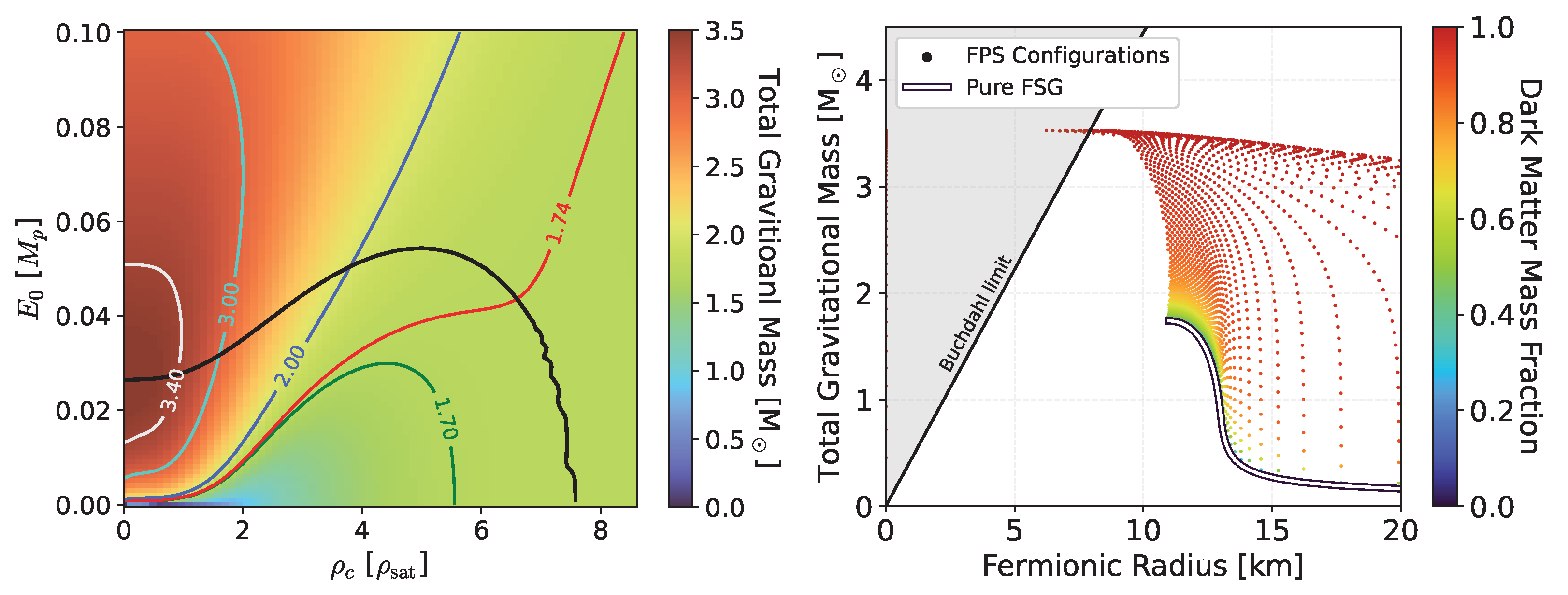