Effective Field Theories


1
Budker Institute of Nuclear Physics, 630090 Novosibirsk, Russia
2
Department of Physics, Novosibirsk State University, 630090 Novosibirsk, Russia
Particles 2020, 3(2), 245-271; https://doi.org/10.3390/particles3020020
Submission received: 2 January 2020
/
Revised: 18 March 2020
/
Accepted: 19 March 2020
/
Published: 31 March 2020
(This article belongs to the Special Issue Quantum Field Theory at the Limits: From Strong Fields to Heavy Quarks)
Abstract
This paper represents a pedagogical introduction to low-energy effective field theories. In some of them, heavy particles are “integrated out” (a typical example—the Heisenberg–Euler EFT); in some, heavy particles remain but some of their degrees of freedom are “integrated out” (Bloch–Nordsieck EFT). A large part of these lectures is, technically, in the framework of QED. QCD examples, namely decoupling of heavy flavors and HQET, are discussed only briefly. However, effective field theories of QCD are very similar to the QED case, and there are just some small technical complications: more diagrams, color factors, etc. The method of regions provides an alternative view at low-energy effective theories; this is also briefly introduced.
1. Introduction
We do not know all physics up to infinitely high energies (or down to infinitely small distances). Therefore, all our theories are effective low-energy (or large-distance) theories (except The Theory of Everything if such a thing exists).
There is a high energy scale M (and a short distance scale ) where an effective theory breaks down. We want to describe light particles (with masses ) and their interactions at low energies, i.e., with characteristic momenta (or, equivalently, at large distances ). To this end, we construct an effective Lagrangian containing the light fields. Physics at small distances produces local interactions of these fields. The Lagrangian contains all possible operators (allowed by symmetries of our theory). Coefficients of operators of dimension are proportional to . If M is much larger than energies we are interested in, we can retain only renormalizable terms (dimension 4), and, perhaps, a power correction or two.
2. Heisenberg–Euler EFT, Heavy Flavors in QCD
A low-energy effective Lagrangian has been first constructed [3,4] to describe photon–photon scattering at . It contained dimension 8 operators made of four . Later an effective Lagrangian for arbitrarily strong homogeneous electromagnetic field has been constructed [5]. It contained all powers of but no terms with derivatives. It is not quite EFT in the modern sense: for each dimensionality not all possible operators are included. In QCD with a heavy flavor with mass M, processes with characteristic energies can be described by an effective Lagrangian without this flavor.
2.1. Photonia
Let us imagine a country, Photonia, in which physicists have high-intensity sources and excellent detectors of low-energy photons, but they do not have electrons and do not know that such a particle exists. (We indignantly refuse to discuss the question “What the experimentalists and their apparata are made of?” as irrelevant.) At first their experiments (Figure 1a) show that photons do not interact with each other. They construct a theory, Quantum PhotoDynamics (QPD), with the Lagrangian
However, later, after they increased the luminosity (and energy) of their “photon colliders” and the sensitivity of their detectors, they discover that photons do scatter, though with a very small cross-section (Figure 1b). They need to add some interaction terms to this Lagrangian.
There are no dimension 6 gauge-invariant operators, because
(this algebraic fact reflects C-parity conservation). All operators with derivatives reduce to
plus full derivatives; this operator vanishes due to equations of motion . On-shell matrix elements of such operators vanish; therefore, we may omit them from the Lagrangian without affecting the S-matrix.
Interaction operators first appear at dimension 8:
Hence the QPD Lagrangian which incorporates the photon–photon interaction is
where the coefficients , M is some large mass (the scale of new physics). Of course, operators of dimensions can be also included, multiplied by higher powers of , but their effect at low energies is much smaller. Physicists from Photonia can extract the two parameters from two experimental results, and predict results of infinitely many measurements.
We are working at the order ; therefore, the photon–photon interaction vertex can appear in any diagram at most once. The only photon self-energy diagram vanishes:
 Therefore, the full photon propagator is equal to the free one. There are no loop corrections to the 4-photon vertex, and hence the interaction operators (4) do not renormalize.

2.2. Qedland
In the neighboring country Qedland physicists are more advanced. In addition to photons, they know electrons and positrons, and investigate their interactions at energies (M is the electron mass). They have constructed a nice theory, QED, which describe their experimental results. (They do not know muons, but this is another story.)
Physicists from Qedland understand that QPD constructed in Photonia is just a low-energy approximation to QED. The coefficients can be calculated by matching. We calculate the amplitude of photon–photon scattering at low energies in the full theory (QED), expanded in the external momenta up to the 4-th order, and equate it to the same amplitude in the effective theory (QPD):


After expanding the QED diagrams in the external momenta they reduce to the vacuum integrals


This QED scattering amplitude is finite at . To reproduce it, the interaction term in the QPD Lagrangian (5) must be [3,4]
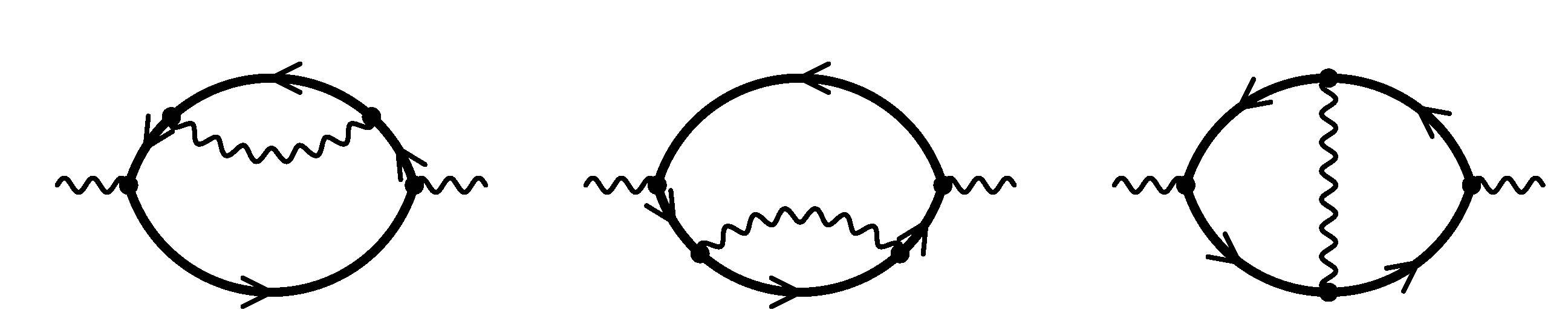
It is not difficult to calculate the two-loop correction to the Lagrangian (9). The two-loop scattering amplitude in QED reduces to the two-loop vacuum integrals
 ( is assumed in all denominators).

2.3. Coulomb Potential
Let us suppose that physicists in Photonia have some classical (infinitely heavy) charged particles, and can manipulate them at their will. If a particle with charge moves along a world line l, the action contains the interaction term
in addition to the photon field action. The integrand in the Feynman path integral contains a phase factor
called the Wilson line. The vacuum-to-vacuum transition amplitude in the presence of classical charges is thus the vacuum average of the corresponding Wilson lines. (In Section 3.2 we will see that the propagator of a heavy charged particle in the effective theory which describes its interaction with soft photons is the straight Wilson line.)
Suppose two charges e and stay at rest at some distance during some (large) time T. The energy of this system is — the interaction potential of the charges. The vacuum transition amplitude is
 (we do not care what happens near its lower and upper ends because ).

The zeroth-order term in the vacuum average of any Wilson loop is 1. It is convenient (though not necessary) to use the Coulomb gauge to calculate the first correction. In this gauge, there is Coulomb photon with the propagator
(it propagates instantaneously) and transverse photon with the propagator
Wilson lines along the 0 direction only interact with Coulomb photons. The self-energy of the classical particle vanishes:
 because the particle propagates along time, and the Coulomb photon along space.

Therefore, there is just one contribution at the order :
 (integration in gives T). Comparing it with (13), we obtain the Fourier transform of the potential
at the Coulomb potential is
(integration in gives T). Comparing it with (13), we obtain the Fourier transform of the potential
at the Coulomb potential is

What about corrections? Vertex corrections vanish for the same reason as (16); crossed-box diagrams vanish because Coulomb photons propagate instantaneously, and the time orderings of the vertices on the left line and on the right one cannot be opposite:


We do not need two-particle-reducible diagrams like
 because they match higher orders of expansion of the exponent (13). Only corrections to the photon propagator can contribute. However, there are no such corrections in QPD. Hence the Coulomb potential (19) is exact in this theory.

In the presence of sources of the photon field, the dimension 6 operator O (3) cannot be ignored. The QPD Lagrangian now contains an extra term
where by dimensionality. This term produces the contribution to the photon self-energy


The aim of an effective theory is to reproduce the S-matrix, so, we may neglect operators vanishing due to equations of motion (in particular, the self-energy (23) vanishes at the photon mass shell , but is needed in a virtual photon line exchanged between classical sources). Therefore, the term (22) reduces to , where is the external (classical) current. For the classical charges e and , it leads to the contact interaction
(It is difficult to observe a -function potential in the interaction of classical charged particles. However, this interaction is essential if the particles are quantum-mechanical—it shifts energies of S-wave states.)
What can physicists in Qedland say about the interaction potential between classical charged particles? In QED, the photon self-energy is gauge invariant because there are no off-shell charged external lines. We can use the covariant-gauge self-energy in the Coulomb-gauge propagator:
In macroscopic measurements the potential at is obtained:
Here is the charge in the on-shell renormalization scheme. The term in determines the contact interaction constant c (24).
In the on-shell renormalization scheme
By definition, in this scheme the renormalized propagators near the mass shell are free. In particular,
so that
Another widely used renormalization scheme is :
where all renormalization constants are minimal
and
(where is the Euler constant). The renormalization constant is determined by the condition that the renormalized photon propagator is finite at :
The (32) satisfies the renormalization group equation
Similarly, the renormalized photon field (30) satisfies the renormalization group equation
In QED (34)
2.4. Charge Decoupling
Now we shall discuss the relation between the full theory (QED) and the low-energy effective theory (QPD) more systematically. All QPD quantities will be denoted by primes. In this theory charge is not renormalized:
The macroscopically measured charge is the same in QED and QPD:
The bare charges in the two theories are related by the bare decoupling coefficient:
The charges are related by the renormalized decoupling coefficient:
The photon self-energy in the 1-loop approximation is


Expanding in q and using (8), we obtain
where is the bare electron mass. The correction can be used to obtain the contact interaction c (24); from now on we shall neglect it. The on-shell charge renormalization constant (29) is
The renormalized decoupling coefficient (41) must be finite, and hence the charge renormalization constant is
As a free bonus, we have obtained the QED function (35):
the negative sign corresponds to screening. (The photon self-energy can be written as a dispersion integral with a positive spectral density. Therefore, the potential (25) up to 1 loop is a superposition of the Coulomb potential and Yukawa ones having various radii, with positive weights. The farther we are from the source, the more Yukawa potentials die out, and the weaker is the interaction.) The renormalized charge decoupling coefficient expressed via the renormalized and electron mass is
where
In the 1-loop term we need the 1-loop (45) and the 1-loop mass renormalization constant defined by
The 1-loop on-shell renormalization constant can be easily calculated using the on-shell integrals


The result is
Both and are finite at , hence
Now we have expressed via the renormalized quantities , . The renormalized decoupling coefficient (41) must be finite, and hence we obtain the 2-loop charge renormalization constant
(by the way, it gives ). The renormalized charge decoupling coefficient is
If we define as the root of the equation
then at , and
Please note that the 1-loop term is needed in 2-loop calculations, because it can get multiplied by an divergent 1-loop integral.
For any , ; if we choose, say, or , there will be a finite correction of order .
More details about decoupling can be found, e.g., in the review [6].
2.5. Qedland Again
Physicists in Qedland suspect that QED is also only a low-energy effective theory. We know that they are right, and muons exist. (In our real world ; for simplicity we shall assume that pions and other light hadrons do not exist.) There are two ways in which they can search for new physics:
- by increasing the energy of their colliders in the hope to produce pairs of new particles;
- by performing high-precision experiments at low energies (e.g., by measuring the electron magnetic moment).
New physics can produce new local interactions of photons, electrons, and positrons at low energies, which should be included in the effective QED Lagrangian. We were lucky that the scale of new physics in QED, the muon mass M, is far away from the electron mass: . Contributions of muon loops to low-energy processes are also strongly suppressed by powers of . Therefore, the prediction for the electron magnetic moment from the pure QED Lagrangian (without non-renormalizable corrections) is in good agreement with experiment.
After this spectacular success of the simplest Dirac equation (without the Pauli term) for electrons, physicists expected that the same holds for the proton, and its magnetic moment is . No luck here. This shows that the picture of the proton as a point-like structureless particle is a poor approximation already at the energy scale .
2.6. Heavy Flavors in QCD
In QED, effects of decoupling of muon loops are tiny. Also, pion pairs become important at about the same energies as muon pairs, so that QED with electrons and muons is a model with a narrow region of applicability. In QCD, decoupling of heavy flavors is fundamental and omnipresent. It would be a huge mistake to use the full 6-flavor QCD at characteristic energies of order GeV: running of and other quantities would be grossly inadequate, convergence of perturbative series would be awful because of large logarithms. In most cases, everybody working in QCD uses an effective low-energy theory, where a few heaviest flavors have been eliminated (even if he does not know that he speaks prose).
Let us consider QCD with a single heavy flavor with mass M; for simplicity, all other flavors are supposed to be massless. Then the behavior of light quarks and gluons at low momenta is described by the low-energy effective theory. Its Lagrangian is the usual QCD Lagrangian (of course, without the heavy-quark field) plus higher-dimensional terms (whose coefficients are suppressed by powers of ). Power corrections to the Lagrangian first appear at dimension 6.
The full-QCD coupling is related to the effective-theory coupling by the decoupling coefficient
Here the term can be obtained from the QED result (57) by inserting the obvious color factors; the term needs a new calculation. The decoupling coefficient for any can be found by solving the renormalization group equation
with the initial condition (60).
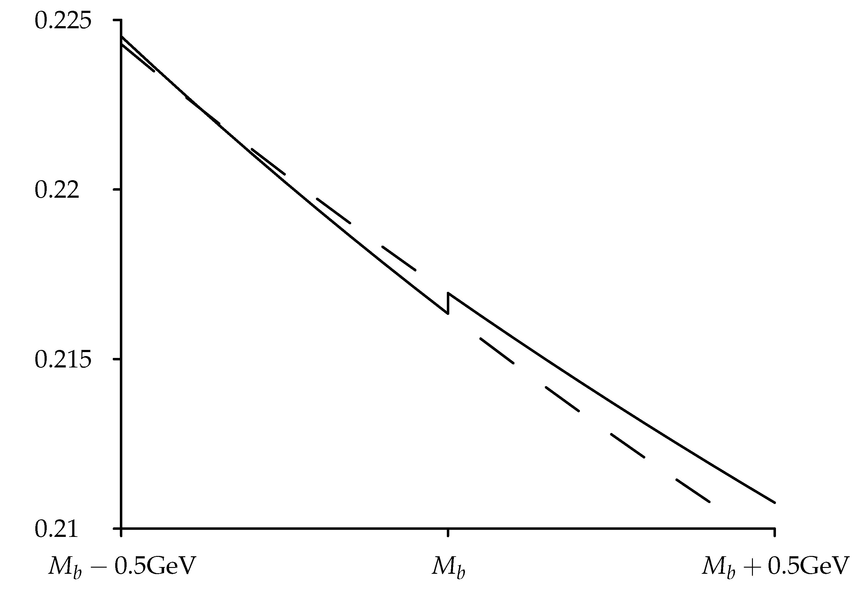
The QCD running coupling not only runs when varies; it also jumps when crossing heavy-flavor thresholds. The behavior of near is shown in Figure 3. At , the correct theory is the full 5-flavor QCD (, the solid line); at , the correct theory is the effective low-energy 4-flavor QCD (, the solid line); the jump at is shown. Of course, both curves can be continued across (dashed lines), and it is inessential at which particular we switch from one theory to the other one. However, the on-shell mass (or any other mass which differs from it by , such as, e.g., ) is most convenient, because the jump is small, . For, say, or , it would be .
We do not discuss another important effective field theory here. Weak interactions at low energies can be described by an effective theory which does not contain W, Z and other heavy particles (Higgs, t). Its Lagrangian contains four-fermion interaction operators (and some other dimension 6 terms). Essentially, it is the weak interaction theory proposed by Fermi [10] and improved by Feynman, Gell-Mann [11] and Marshak, Sudarshan [12]. It is discussed, e.g., in lectures [13,14].
2.7. Method of Regions
This method (see the textbook [15]) provides an alternative insight to effective field theories. It allows one to calculate diagrams expanded in small ratios of scales directly. It is convenient when you need to calculate a small number of diagrams expanded up to a high order in a small parameter, because effective Lagrangians quickly become very long at such high orders. On the other hand, effective Lagrangians are applicable for all processes, and are useful for investigation general properties (symmetries, factorization).
Let us consider the vacuum integral
 with two masses M and m at and . It contains neither ultraviolet (UV) nor infrared (IR) divergences. After Wick rotation to Euclidean momentum space it becomes

Of course, in this simple example it is easy to obtain the exact solution. We use partial fraction decomposition


These two integrals, taken separately, diverge; therefore, we use dimensional regularization () and obtain
This result is finite at :
It is easier to obtain this result using the prescription known as the method of regions. The integral (62) is written at the sum of contributions of two regions, the hard one and the soft one:
In the hard region ; in the soft one . The integrand is expanded to Taylor series in accordance to these power counting rules in each region. After that, the integral is taken over the full (d-dimensional) space.
In the hard region () we have
where the operator expands the integrand in small parameter(s) counting as a quantity of order M:
Calculating the loop integrals, we arrive at
The result is a Taylor series in m. Each loop integral is IR divergent; it contains a single scale M, and hence, by dimensions counting, is proportional to .
In the soft region () we have
where counts as a quantity of order m:
and we obtain
The result is a Taylor series in . Each loop integral is UV divergent; it contains a single scale m, and hence, by dimensions counting, is proportional to .
The sum of the hard contribution (64) and the soft one (65) produces the complete result (63). IR divergences in the hard region cancel UV divergences in the soft one.
In this simple case it is easy to prove this prescription [16]. Let us introduce some boundary such that , and write
We may apply to the first integrand and to the second one:
For each of these two integrals, we add and subtract the integral over the remaining part of the space:
where
are the integrals of the two expansions over the “wrong” parts of the space. In these wrong regions, we may apply the other expansion in addition to the existing one:
However, this is the integral over the full space:
because the Taylor expansion operators commute:
And hence
because each integral has no scale.
Let us stress that the method of regions works thanks to dimensional regularization. Taylor expansions in each region (i.e., for each set of power counting rules) must be performed completely, up to the end; otherwise, integrals in the defect can contain some scale(s), and hence not vanish.
Let us consider QCD with light flavors and a heavy flavor of mass M, and calculate some scattering amplitude of light quarks and gluons with low characteristic energies . We can use the method of regions. For each diagram, some subdiagrams will be hard (characteristic momenta ; in particular, all heavy-quark loops are in such subdiagrams); light-quark and gluon lines connecting these hard subdiagrams will be soft (characteristic momenta ). In the EFT language, these hard subdiagrams are local interactions present in the effective Lagrangian; the overall soft diagram is calculated according to the Feynman rules of the low-energy theory.
3. Bloch–Nordsieck EFT, HQET
In the previously considered effective field theories heavy particles are completely absent in the effective Lagrangians. There is another kind of effective theories in which heavy particles are retained, but move non-relativistically in some reference frame and can be described in a simplified way. This effective theory has been first constructed by Bloch and Nordsieck [17] to describe interaction of an electron with soft photons. Its non-abelian version is called heavy quark effective theory (HQET), see, e.g., [18,19,20,21]. It is used to describe properties of hadrons with a single heavy quark in QCD.
3.1. Heavy Electron Effective Theory
Photonia has imported a single electron from Qedland, and physicists are studying its interaction with soft photons (both real and virtual) which they can produce and detect so well. The aim is to construct a theory describing states with a single electron plus soft photon fields.
The ground state (“vacuum”) of the theory is the electron at rest (and no photons). It is natural to define its energy to be 0. When the electron has momentum , its energy is
where M is the electron mass (in the on-shell renormalization scheme), our large mass scale. The electron velocity is
At the leading (0-th) order in , the mass shell of the free electron is
At this order, the electron velocity is
The electron does not move; it always stays in the point where it has been put initially. The Lagrangian
where h is the 2-component spinor electron field, leads to the equation of motion
This means that the energy of an on-shell electron is . Thus, the Lagrangian (70) reproduces the mass shell (68), and can be used to describe the free electron at the leading order in .
The electron has charge . Therefore, when placed in an external electromagnetic field, it has energy
instead of (68). Therefore, the equation of motion is
instead of (71), where
is the covariant derivative. It can be obtained from the HEET Lagrangian [22]
This Lagrangian is not Lorentz-invariant. It is invariant with respect to the gauge transformation
Of course, the full Lagrangian is the sum of (75) and the Lagrangian of the photon field. This gives the equation of motion for the electromagnetic field
where the current has only 0-th component
(the interaction term in the Lagrangian (75) is ). The electron produces the Coulomb field.
At the leading order in , the electron spin does not interact with electromagnetic field. We can rotate it without affecting physics. Speaking more formally, the Lagrangian (75) has, in addition to the symmetry , also the spin symmetry [23]: it is invariant with respect to transformations
where U is a matrix ().
In fact, the electron has magnetic moment proportional to its spin , and this magnetic moment interacts with magnetic field: the interaction Hamiltonian is . However, by dimensionality the magnetic moment , and this interaction only appears at the level of corrections. Specifically, (up to small radiative corrections), where
is the Bohr magneton. The Lagrangian thus has an additional term describing this magnetic interaction,
This term violates the spin symmetry at the level.
If we assume that there are flavors of heavy fermions,
then the Lagrangian has symmetry (even when the masses are different). The spin-flavor symmetry is broken at the level by both the kinetic-energy term and the magnetic-interaction term.
At the leading order in , not only the spin direction but also its magnitude is irrelevant. We can, for example, switch the electron spin off:
where is a scalar field (with charge ). This is the most convenient form of the Lagrangian in all cases when we are not interested in corrections. If we consider the scalar and the spinor fields together,
then this Lagrangian has symmetry [24]. The superflavor symmetry contains, in addition to spin transformations (79) and phase rotations , , also transformations which mix spin-0 and spin- fields. In the infinitesimal form,
where is an infinitesimal spinor parameter. Therefore, this is a supersymmetry group. If we want, we can consider, e.g., spins and 1; the corresponding Lagrangian has superflavor symmetry. The superflavor symmetry is broken at the level by the magnetic-interaction term in the Lagrangian (81).
3.2. Feynman Rules
For now, we are working at the leading order in . The HEET Lagrangian expressed via the bare fields and parameters is
It gives the usual photon propagator. From the free electron part we obtain the momentum-space free electron propagator


It depends only on , not on . If we use the spin- field instead of the spin-0 field , then the unit spin matrix is assumed here. The coordinate-space propagator is its Fourier transform:


The infinitely heavy (static) electron does not move: it always stays at the point where it has been placed initially. Alternatively, instead of Fourier-transforming (87), we can obtain (88) by direct solving the equation
for the free x-space propagator. Finally, the interaction term in (86) produces the vertex
 where
is the 4-velocity of our laboratory frame (in which the electron is nearly at rest all the time).
where
is the 4-velocity of our laboratory frame (in which the electron is nearly at rest all the time).

The static field (or ) describes only particles, there are no antiparticles. Therefore, there are no pair creation and annihilation (even virtual). In other words, there are no loops formed by propagators of the static electron. The electron propagates only forward in time (88); the product of functions along a loop vanishes. We can also see this in momentum space: all poles of the propagators (87) in such a loop are in the lower half-plane, and closing the integration contour upwards, we get 0.
It is easy to find the propagator of the static electron in an arbitrary external electromagnetic field . It satisfies the equation
instead of (89) (the derivative acts on x). Its solution is
where
is the straight Wilson line from to x (along v). The same formula can be used when the electromagnetic field is quantum (operator ), but the exponent (94) must be path-ordered: operators referring to earlier points (along the path) are placed to the right from those for later points. This is usually denoted by ; when the path is directed to the future, P-ordering coincides with T-ordering. The Wilson line has a useful property
Properties of Wilson lines were investigated in many papers, see, e.g., [25,26]. Many results now considered classics of HQET were derived in the course of these studies before HQET was invented in 1990. In particular, the HQET Lagrangian (83) has been introduced as a technical device for investigation of Wilson lines.
The lowest-energy state (“vacuum”) in HEET is a single electron at rest, and it is convenient to use its energy as the zero level. In the full theory, its energy is M, and
where E is the energy of some state (containing a single electron) in the full theory, and is its energy in HEET (it is called the residual energy). We can re-write this relation in a relativistic form:
where is the 4-momentum of some state (containing a single electron) in the full theory, is its momentum in HEET (the residual momentum), and is 4-velocity of a reference frame in which the electron always stays approximately at rest. In other words, HEET is applicable if there exists such a 4-velocity v that, after decomposition (97), the components of the electron residual momentum p are always small, and components of all photon momenta are also small:
This condition does not fix v uniquely; it can be varied by . Effective theories corresponding to different choices of v must produce identical physical predictions. This requirement is called reparameterization invariance [27]. It produces relations between some quantities of different orders in .
This Lagrangian is not Lorentz-invariant, because it contains a fixed vector v. It gives the free propagator
The mass shell of the static electron is
If we want to consider the spin- electron, it is described by the 4-component (Dirac) spinor field which satisfies the condition
(so that in the v rest frame the field has only 2 upper components non-vanishing). The Lagrangian [28,29]
gives the propagator
and the vertex (90).
And what can our friends from Qedland say about this theory? They are not surprised. The finite-mass free electron propagator with (97), can be approximated as
Diagrammatically, it is related to the HEET propagator:


When a QED vertex is sandwiched between two propagators (104), it can be replaced by the HEET vertex :
What if there is an external spinor after the vertex (or before it)? From the Dirac equation we have
so that we may insert the projectors before and after , too, and the replacement (107) is applicable. We have derived the HEET Feynman rules from the QED ones in the limit . Therefore, we again arrive at the HEET Lagrangian (103) which corresponds to these Feynman rules.
We have thus proved that at the tree level any QED diagram is equal to the corresponding HEET diagram up to corrections. This is not true at loops, because loop momenta can be arbitrarily large. Renormalization properties of HEET (anomalous dimensions, etc.) differ from those in QED. QED loop diagrams can be decomposed into integration regions (Section 2.7), with some loops hard (momenta ) and some soft (momenta ). Then hard loops produce local interactions (in the effective theory language, they follow from local operators in the HEET Lagrangian); soft loops can be calculated as in HEET.
3.3. The Heavy Propagator and Current
In fact, the static-electron propagator can be calculated exactly [30]! Suppose we calculate the one-loop correction to the static-electron propagator in coordinate space. Let us multiply this correction by itself. We obtain an integral in , , , with , . The ordering of primed and non-primed integration times can be arbitrary. The integration area is subdivided into six regions, corresponding to the six diagrams:


This is twice the 2-loop correction to the propagator. Continuing this drawing exercise, we see that the one-loop correction cubed is times the 3-loop correction, and so on. Therefore, the exact all-order propagator is the exponential of the one-loop correction:
(). In particular, in the d-dimensional Yennie gauge [31]
the exact propagator (109) is free.
There are no corrections to the photon propagator in HEET (86) because static-electron loops do not exist. (This argument works up to the order . At a 4-photon interaction appears, see Section 2.1. However, the only correction to the photon propagator at this order vanishes (6). The first non-vanishing correction involves two 4-photon vertices, and appears at .) Therefore, the photon field renormalization constant , and hence , . The renormalization constant of the static-electron field h and its anomalous dimension are thus known exactly:
Suppose the electron substantially changes its 4-velocity (due to some hard-photon interaction). In the HEET framework this can be described by the current (Figure 4)
where . Its anomalous dimension
is called the cusp anomalous dimension. If () then and . Exponentiation works for Wilson lines of any shape, in particular, lines with a cusp. Therefore, the 1-loop formula for is exact.
There are many methods to calculate . The simplest one is based on unitarity. The electron after the kick either remains itself (probability , where F is its form factor) or emits one or several protons:
Up to the first order in ,


In classical electrodynamics the spectrum of emitted radiation is [32,33]
and hence the probability of photon emission is
In dimensional regularization, by dimensions counting, this probability becomes
(up to a factor which tends to 1 at ; we do not need such a factor). Hence the form factor is
where is an infrared cutoff. We need only the ultraviolet divergence of F, and so we must introduce such a cutoff. We obtain
and
It is given by the soft radiation function in classical electrodynamics, and should be included in The Guinness Book of Records as the anomalous dimension known for the longest time (probably, years).
3.4. Hadrons with a Heavy Quark
The B meson is the hydrogen atom of quantum chromodynamics, the simplest non-trivial hadron. In the leading approximation, the b quark in it just sits at rest at the origin and creates a chromoelectric field. Light constituents (gluons, light quarks and antiquarks) move in this external field. Their motion is relativistic; the number of gluons and light quark–antiquark pairs in this light cloud is undetermined and varying. Therefore, there are no reasons to expect that a non-relativistic potential quark model would describe the B meson well enough (in contrast to the meson, where the non-relativistic two-particle picture gives a good starting point).
Similarly, the baryon can be called the helium atom of QCD. Unlike in atomic physics, where the hydrogen atom is much simpler than helium, the B and are equally difficult. Both have a light cloud with a variable number of relativistic particles. The size of this cloud is the confinement radius ; its properties are determined by large-distance nonperturbative QCD.
The analogy with atomic physics can tell us a lot about hadrons with a heavy quark. The usual hydrogen and tritium have identical chemical properties, even though the tritium nucleus is three times heavier than the proton. Both nuclei create identical electric fields, and both stay at rest. Similarly, the D and B mesons have identical “hadro-chemical” properties, even though the b quark is three times heavier than the c.
The proton magnetic moment is of the order of the nuclear magneton , and is much smaller than the electron magnetic moment . Therefore, the energy difference between the states of the hydrogen atom with total spins 0 and 1 (hyperfine splitting) is small (of the order times the fine structure). Similarly, the b-quark chromomagnetic moment is proportional to by dimensionality, and the hyperfine splitting between the B and mesons is small (proportional to ). Unlike in atomic physics, both “gross”-structure intervals and fine-structure intervals are just some numbers times , because the light components are relativistic (the practical success of constituent quark models shows that these dimensionless numbers for fine splittings can be rather small, but they contain no small parameter).
In the limit , the heavy-quark spin does not interact with the gluon field. Therefore, it may be rotated at will, without changing the physics. Such rotations can transform the B and into each other; they are degenerate and have identical properties in this limit. This heavy-quark spin symmetry yields many useful relations among heavy-hadron form factors. Not only the orientation, but also the magnitude of the heavy-quark spin is irrelevant in the infinite-mass limit. We can switch off the heavy-quark spin, making it spinless, without affecting the physics. This leads to a supersymmetry group called the superflavor symmetry. It can be used to predict properties of hadrons containing a scalar or vector heavy quark. Such quarks exist in some extensions of the Standard Model (for example, supersymmetric or composite extensions).
This idea can also be applied to baryons with two heavy quarks. They form a small-size bound state (with a radius of order ) which has spin 0 or 1 and is antitriplet in color. Therefore, these baryons are similar to mesons with a heavy antiquark that has spin 0 or 1. The accuracy of this picture cannot be high, however, because even the radius of the diquark is only a few times smaller than the confinement radius.
Let us consider mesons with the quark contents , where Q is a heavy quark with mass M (b or c), and q is a light quark (u, d, or s). As discussed above, the heavy-quark spin is inessential in the limit , and may be switched off. In a world with a scalar heavy antiquark, S-wave mesons have angular momentum and parity ; P-wave mesons have and . The energy difference between these two P-wave states (fine splitting) is a constant times at , just like the splittings between these P-wave states and the ground state; however, this constant is likely to be small.
In our real world, the heavy antiquark has spin and parity . The quantum numbers in the above paragraph are those of the cloud of light fields of a meson. Adding the heavy-antiquark spin, we obtain, in the limit , a degenerate doublet of S-wave mesons with spin and parity and , and two degenerate doublets of P-wave mesons, one with and , and the other with and . At a large but finite heavy-quark mass M, these doublets are not exactly degenerate. Hyperfine splittings, equal to some dimensionless numbers times , appear. It is natural to expect that hyperfine splittings in P-wave mesons are less than in the ground-state S-wave doublet, because the characteristic distance between the quarks is larger in the P-wave case. Please note that the mesons from the different doublets do not differ from each other by any exactly conserved quantum numbers, and hence can mix. They differ by the angular momenta of the light fields, which is conserved up to corrections; therefore, the mixing angle should be of the order of .
Mesons with and d form isodoublets; together with isosinglets with , they form triplets.
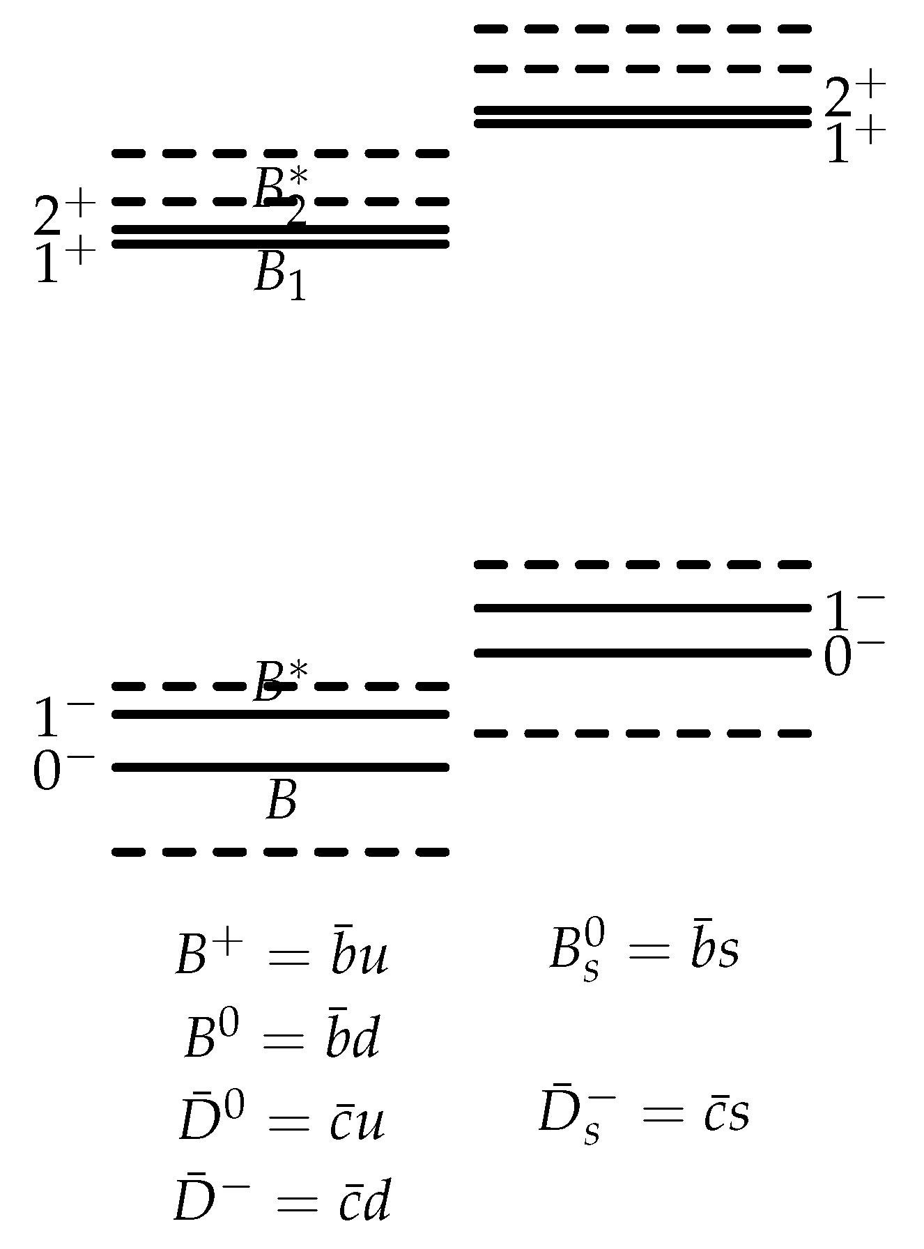
The experimentally observed mesons containing the antiquark are shown in Figure 5. The mesons and form a doublet, with the quantum numbers of the light fields . The second P-wave doublet with is suspiciously absent. The mesons decays into the ground-state doublet and a meson in D-wave (); the pion momentum is small, these decays are strongly suppressed, and the mesons are narrow. The mesons decays into the ground-state ones and a meson in S-wave (); these decays are not suppressed, and hence the mesons are very wide. Hyperfine splitting of the P-wave doublet is smaller than that of the S-wave one.
In the leading approximation, the spectrum of -containing mesons is obtained from the spectrum of -containing mesons simply by a shift by . The spectrum of mesons containing is also shown in Figure 5. It is positioned in such a way that the weighted average energies of the ground-state doublets and coincide. Hyperfine splittings are smaller for B mesons than for D mesons, as expected.
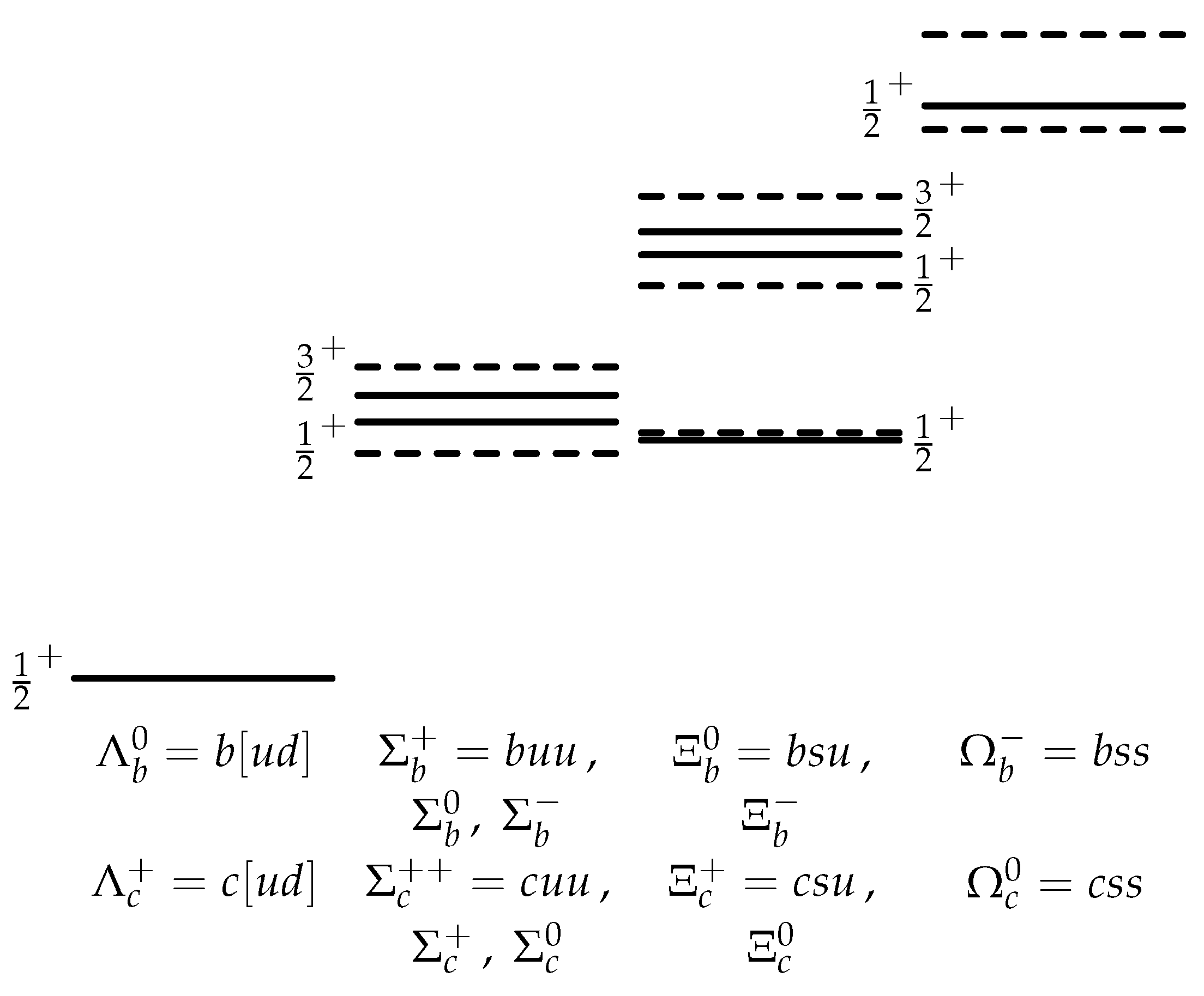
In S-wave baryons, the light-quark spins can add to give or . In the first case their spin wave function is antisymmetric; the Fermi statistics and the antisymmetry in color require an antisymmetric flavor wave function. Hence the light quarks must be different; if they are u, d, then their isospin is . With the heavy-quark spin switched off, this gives the baryon with . If one of the light quarks is s, we have the isodoublet , which forms an antitriplet together with . With the heavy-quark spin switched on, these baryons have . In the case, the flavor wave function is symmetric. If the light quarks are u, d, then their isospin is . This gives the isotriplet ; with one s quark, we obtain the isodoublet ; and with two s quarks, the isosinglet . Together, they form an sextet. With the heavy-quark spin switched on, we obtain the degenerate doublets with , : , ; , ; , . The hyperfine splittings in these doublets are of the order of . Mixing between and is suppressed both by and by .
The experimentally observed baryons containing b are shown in Figure 6. In the third column, the lowest state is followed by the doublet , . The baryon has not yet been observed. The spectrum of baryons containing c is also shown. It is positioned in such a way that the ground-state baryons and coincide.
In the leading approximation, the masses and are both equal to , where is the energy of the ground state of the light fields in the chromoelectric field of the antiquark. This energy is of the order of . The excited states of the light fields have energies , giving excited degenerate doublets with masses .
There are two corrections to the masses. First, the antiquark has an average momentum squared , which is of order of . Therefore, it has a kinetic energy . Second, the chromomagnetic moment interacts with the chromomagnetic field created by light constituents at the origin, where the stays. This chromomagnetic field is proportional to the angular momentum of the light fields . Therefore, the chromomagnetic interaction energy is proportional to
where is the meson spin. If we denote this energy for B by , then for it will be . Here is of order of . The B, meson masses with corrections taken into account are given by the formulae
The hyperfine splitting is
Taking into account , we obtain
The difference is given by a similar formula, with instead of . Therefore, the ratio
Experimentally, this ratio is 0.88. This is a spectacular confirmation of the idea that violations of the heavy-quark spin symmetry are proportional to .
Let us now discuss the B-meson leptonic decay constant . It is defined by
where the one-particle state is normalized in the usual Lorentz-invariant way:
This relativistic normalization becomes nonsensical in the limit , and in that case the non-relativistic normalization
should be used instead. Then, for the B meson at rest,
Denoting this matrix element (which is mass-independent at ) by , we obtain
and hence
HQET (or HEET) is applicable to problems with a single heavy particle. In the leading order this particle moves along a straight world line. Physics of bound states of heavy particles (positronium, heavy quarkonium) is essentially different. In this case, these particles rotate around each other. Their characteristic residual energy is while their characteristic momentum is (where ). Such problems are described by another effective theory—pNRQCD (potential non-relativistic QCD); in the abelian case it is called pNRQED. This theory is in many respects similar to HQET, but is more complicated because of this anisotropy. We do not discuss it here, see, e.g., the reviews [34,35].
Another important EFT which is not discussed here is SCET — Soft-Collinear Effective Theory. It has been first proposed as an effective field theory describing inclusive B meson decays with an energetic light quark in the final state (SCET-I) and exclusive B decays with an energetic light hadron in the final state (SCET-II). Physics at short distances () is encapsulated in matching coefficients; soft dynamics of the b quark is described by HQET; soft and collinear degrees of freedom of light quarks and gluons are described by SCET. Later SCET was successfully applied to numerous problems in hadron collider physics. In this area there are at least two large nearly light-like momenta, and hence several collinear regions (jets, initial hadrons). This theory is discussed in the textbook [36] and lecture courses, e.g., [37,38,39].
4. Conclusions
In the past only renormalizable theories were considered well-defined: they contain a finite number of parameters, which can be extracted from a finite number of experimental results and used to predict results of an infinite number of other potential measurements. Non-renormalizable theories were rejected because their renormalization at all orders in non-renormalizable interactions involve infinitely many parameters, so that such a theory has no predictive power. This principle is absolutely correct, if we are impudent enough to pretend that our theory describes the Nature up to arbitrarily high energies (or down to arbitrarily small distances).
At present we accept the fact that our theories only describe the Nature at sufficiently low energies (or sufficiently large distances). They are effective low-energy theories. Such theories contain all operators (allowed by the relevant symmetries) in their Lagrangians. They are necessarily non-renormalizable. This does not prevent us from obtaining definite predictions at any fixed order in the expansion in , where E is the characteristic energy and M is the scale of new physics. Only if we are lucky and M is many orders of magnitude larger than the energies we are interested in, we can neglect higher-dimensional operators in the Lagrangian and work with a renormalizable theory.
We can add higher-dimensional contributions to the Lagrangian, with further unknown coefficients. To any finite order in , the number of such coefficients is finite, and the theory has predictive power. For example, if we want to work at the order , then either a single (dimension 8) vertex or two ones (dimension 6) can occur in a diagram. UV divergences which appear in diagrams with two dimension 6 vertices are compensated by renormalizing these 2 operators plus dimension 8 counterterms. Therefore, the theory can be renormalized. The usual arguments about non-renormalizability are based on considering diagrams with arbitrarily many vertices of non-renormalizable interactions (operators of dimensions ); this leads to infinitely many free parameters in the theory.
The Standard Model does not describe all physics up to infinitely high energies (or down to infinitely small distances). At least, quantum gravity becomes important at the Planck scale. SM does not explain dark matter and baryon asymmetry of the Universe. What can appear at some very short distance scale?
- supersymmetry;
- compositeness;
- extra dimensions;
- non-pointlike objects: strings/superstrings/branes;
- something we cannot imagine at present.
We can construct scenarios for new physics searches based on some known variants of the next theory (more fundamental than SM). I.e. we can investigate some finite number of directions of departure from SM, but an infinite number of directions which we cannot now imagine remain unexplored—this is a set of measure 0. What we need is a systematic model-independent approach for searching of some absolutely unknown new physics at small distances. It produces new local interactions of the SM fields. This approach is called Standard Model Effective Theory (SMEFT), see, e.g., [40,41].
Funding
The work has been supported by the Russian Ministry of Science and Higher Education.
Conflicts of Interest
The authors declare no conflict of interest.
References
- Petrov, A.A.; Blechman, A.E. Effective Field Theories; World Scientific: Singapore, 2016. [Google Scholar]
- Grozin, A.G. Introduction to effective field theories. 1. Heisenberg–Euler effective theory, decoupling of heavy flavours. arXiv 2009, arXiv:0908.4392. [Google Scholar]
- Euler, H.; Köckel, B. Über die Streuung von Licht an Licht nach der Diracschen Theorie. Naturwissenschaften 1935, 23, 246. [Google Scholar] [CrossRef]
- Euler, H. Über die Streuung von Licht an Licht nach der Diracschen Theorie. Ann. Phys. 1936, 26, 398. [Google Scholar] [CrossRef]
- Heisenberg, W.; Euler, H. Folgerungen aus der Diracschen Theorie des Positrons. Z. Phys. 1936, 98, 714. [Google Scholar] [CrossRef]
- Grozin, A.G. Decoupling in QED and QCD. Int. J. Mod. Phys. 2013, A28, 1350015. [Google Scholar] [CrossRef]
- Bernreuther, W.; Wetzel, W. Decoupling of Heavy Quarks in the Minimal Subtraction Scheme. Nucl. Phys. 1982, B197, 228. [Google Scholar] [CrossRef]
- Larin, S.A.; van Ritbergen, T.; Vermaseren, J.A.M. The Large quark mass expansion of Γ(Z0→hadrons) and Γ(τ−→ντ+hadrons) in the order . Nucl. Phys. 1995, B438, 278. [Google Scholar] [CrossRef]
- Chetyrkin, K.G.; Kniehl, B.A.; Steinhauser, M. Decoupling relations to () and their connection to low-energy theorems. Nucl. Phys. 1998, B510, 61. [Google Scholar] [CrossRef]
- Fermi, E. Versuch einer Theorie der β-Strahlen. I. Z. Phys. 1934, 88, 161. [Google Scholar] [CrossRef]
- Feynman, R.P.; Gell-Mann, M. Theory of Fermi interaction. Phys. Rev. 1958, 109, 193. [Google Scholar] [CrossRef]
- Sudarshan, E.C.G.; Marshak, R.E. Chirality invariance and the universal Fermi interaction. Phys. Rev. 1958, 109, 1860. [Google Scholar] [CrossRef]
- Buras, A.J. Weak Hamiltonian, CP violation and rare decays. arXiv 1998, arXiv:hep-ph/9806471. [Google Scholar]
- Grozin, A.G. Effective weak Lagrangians in the Standard Model and B decays. In Proceedings of the Helmholtz International School Physics of Heavy Quarks and Hadrons, Dubna, Russia, 15–28 July 2013; p. 78. [Google Scholar]
- Smirnov, V.A. Applied Asymptotic Expansions in Momenta and Masses; Springer Tracts in Modern Physics 177; Springer: Berlin/Heidelberg, Germany, 2002. [Google Scholar]
- Jantzen, B. Foundation and generalization of the expansion by regions. JHEP 2011, 12, 076. [Google Scholar] [CrossRef]
- Bloch, F.; Nordsieck, A. Note on the Radiation Field of the Electron. Phys. Rev. 1937, 52, 54. [Google Scholar]
- Neubert, M. Heavy Quark Symmetry. Phys. Rep. 1994, 245, 259. [Google Scholar] [CrossRef]
- Manohar, A.V.; Wise, M.B. Heavy Quark Physics; Cambridge University Press: Cambridge, UK, 2000. [Google Scholar]
- Grozin, A.G. Heavy Quark Effective Theory; Springer Tracts in Modern Physics 201; Springer: Berlin/Heidelberg, Germany, 2004. [Google Scholar]
- Grozin, A.G. Higher radiative corrections in HQET. In Proceedings of the Helmholtz Intenrnational School Heavy Quark Physics, Dubna, Russia, 11–21 August 2008; p. 55. [Google Scholar]
- Eichten, E.; Hill, B. An effective field theory for the calculation of matrix elements involving heavy quarks. Phys. Lett. 1990, B234, 511. [Google Scholar] [CrossRef]
- Isgur, N.; Wise, M.B. Weak transition form factors between heavy mesons. Phys. Lett. 1990, B237, 527. [Google Scholar] [CrossRef]
- Georgi, H.; Wise, M.B. Superflavor symmetry for heavy particles. Phys. Lett. 1990, B243, 279. [Google Scholar] [CrossRef]
- Cherednikov, I.O.; Mertens, T.; Van der Veken, F. Wilson Lines in Quantum Field Theory, 2nd ed.; De Gruyter Studies in Mathematical Physics 24; Walter de Gruyter GmbH: Berlin/Boston, Germany, 2020. [Google Scholar]
- Dorn, H. Renormalization of Path Ordered Phase Factors and Related Hadron Operators in Gauge Field Theories. Fortsch. Phys. 1986, 34, 11. [Google Scholar]
- Luke, M.E.; Manohar, A.V. Reparametrization invariance constraints on heavy particle effective field theories. Phys. Lett. 1992, B286, 348. [Google Scholar] [CrossRef]
- Grinstein, B. The static quark effective theory. Nucl. Phys. 1990, B339, 253. [Google Scholar] [CrossRef]
- Georgi, H. An effective field theory for heavy quarks at low energies. Phys. Lett. 1990, B240, 447. [Google Scholar] [CrossRef]
- Yennie, D.R.; Frautschi, S.C.; Suura, H. The infrared divergence phenomena and high-energy processes. Ann. Phys. 1961, 13, 379. [Google Scholar] [CrossRef]
- Fried, H.M.; Yennie, D.R. New Techniques in the Lamb Shift Calculation. Phys. Rev. 1958, 112, 1391. [Google Scholar] [CrossRef]
- Landau, L.D.; Lifshitz, E.M. The Classical Theory of Fields, 4th ed.; The Problem after Section 69; Butterworth-Heinemann: Oxford, UK, 1980. [Google Scholar]
- Jackson, J.D. Classical Electrodynamics, 3rd ed.; Section 15.6; Wiley: Hoboken, NJ, USA, 1999. [Google Scholar]
- Brambilla, N.; Pineda, A.; Soto, J.; Vairo, A. Effective Field Theories for Heavy Quarkonium. Rev. Mod. Phys. 2005, 77, 1423. [Google Scholar] [CrossRef]
- Pineda, A. Review of Heavy Quarkonium at weak coupling. Prog. Part. Nucl. Phys. 2012, 67, 735. [Google Scholar] [CrossRef]
- Becher, T.; Broggio, A.; Ferroglia, A. Introduction to Soft-Collinear Effective Theory; Lecture Notes in Physics 896; Springer: Cham, Switzerland, 2015. [Google Scholar]
- Bauer, C.W.; Stewart, I.W. The Soft-Collinear Effective Theory. Available online: https://courses.edx.org/c4x/MITx/8.EFTx/asset/notes_scetnotes.pdf (accessed on 21 March 2020).
- Grozin, A.G. Lectures on Soft-Collinear Effective Theory. In Proceedings of the Helmholtz International School Quantum Field Theory at the Limits: From Strong Fields to Heavy Quarks, Dubna, Russia, 18–30 July 2016; p. 121. [Google Scholar]
- Becher, T. Les Houches Lectures on Soft-Collinear Effective Theory. arXiv 2018, arXiv:1803.04310. [Google Scholar]
- Grzadkowski, B.; Iskrzyński, B.; Misiak, M.; Rosiek, J. Dimension-six terms in the Standard Model Lagrangian. JHEP 2010, 10, 85. [Google Scholar] [CrossRef]
- Dedes, A.; Materkowska, W.; Paraskevas, M.; Rosiek, J.; Suxho, K. Feynman rules for the Standard Model Effective Field Theory in Rξ-gauges. JHEP 2017, 06, 143. [Google Scholar] [CrossRef]
Figure 1.
Scattering of low-energy photons: (a) not yet seen; (b) observed.

Figure 2.
The 2-loop photon self-energy.

Figure 3.
and .

Figure 4.
Heavy–heavy current.

Figure 5.
Mesons with (solid lines) and (dashed lines).

Figure 6.
Baryons with b (solid lines) and c (dashed lines).

© 2020 by the author. Licensee MDPI, Basel, Switzerland. This article is an open access article distributed under the terms and conditions of the Creative Commons Attribution (CC BY) license (http://creativecommons.org/licenses/by/4.0/).
Share and Cite
MDPI and ACS Style
Grozin, A. Effective Field Theories. Particles 2020, 3, 245-271. https://doi.org/10.3390/particles3020020
AMA Style
Grozin A. Effective Field Theories. Particles. 2020; 3(2):245-271. https://doi.org/10.3390/particles3020020
Chicago/Turabian StyleGrozin, Andrey. 2020. "Effective Field Theories" Particles 3, no. 2: 245-271. https://doi.org/10.3390/particles3020020
APA StyleGrozin, A. (2020). Effective Field Theories. Particles, 3(2), 245-271. https://doi.org/10.3390/particles3020020