Abstract
We consider the formation of structured and massless particles with spin 1, by using the Yang–Mills-like stochastic equations system for the group symmetry without taking into account the nonlinear term characterizing self-action. We prove that, in the first phase of relaxation, as a result of multi-scale random fluctuations of quantum fields, massless particles with spin 1, further referred as hions, are generated in the form of statistically stable quantized structures, which are localized on 2D topological manifolds. We also study the wave state and the geometrical structure of the hion when as a free particle and, accordingly, while it interacts with a random environment becoming a quasi-particle with a finite lifetime. In the second phase of relaxation, the vector boson makes spontaneous transitions to other massless and mass states. The problem of entanglement of two hions with opposite projections of the spins and and the formation of a scalar zero-spin boson are also thoroughly studied. We analyze the properties of the scalar field and show that it corresponds to the Bose–Einstein (BE) condensate. The scalar boson decay problems, as well as a number of features characterizing the stability of BE condensate, are also discussed. Then, we report on the structure of empty space–time in the context of new properties of the quantum vacuum, implying on the existence of a natural quantum computer with complicated logic, which manifests in the form of dark energy. The possibilities of space–time engineering are also discussed.
1. Introduction
From a mathematical and philosophical point of view, the vacuum can be comparable to the region of absolutely empty space or, equivalently, with the region of the space where there are no fields and massive particles (see for example [1]). One can mention the Lamb Shift [2], Casimir effect [3], Unruh effect [4], anomalous magnetic moment of the electron [5], Van der Waals forces [6], Delbrück scattering [7], Hawking radiation [8], the cosmological constant problem [9,10], and vacuum polarization at weak electromagnetic fields [11,12,13]—here is an incomplete list of phenomena, part of which has been experimentally discovered, which are conditioned by the physical vacuum or, more accurately, by a quantum vacuum (QV). In reference [10] author discuss the issues of cosmic acceleration, while in [14] dark energy-quintessence are studied in the framework of QV theories, which necessarily include scalar fields. In reference [15] authors evaluate mass and electric dipole moment of the graviton, identifying as a particle of dark matter, which radically changes our understanding of dark matter and possibly of dark energy. The properties of QV can be studied in the scope of quantum field theory (QFT), i.e., quantum electrodynamics (QED) and quantum chromodynamics (QCD). Note that QFT may accurately describe QV, considering that one can sum up an infinite series of perturbation theory terms, which is typical of field theories. However, it is well known that perturbation theory for QFT does not converges at low energies, failing to describe, for example, nonzero values of the vacuum expectation, called condensates in QCD or the BCS superconductivity theory. In particular, as shown in [16], as well as in [17], the radiative corrections of the massless Yang–Mills theory leads to instability of the vacuum state, which corresponds to the asymptotic freedom of gauge theories and is due to infrared features.
According to the Standard Model (SM) precisely the non-zero vacuum expectation value of the Higgs field [18,19], arising from spontaneous symmetry breaking, is the principle mechanism allowing the generation of masses.
To overcome these difficulties and conduct a consistent and comprehensive QV study, we propose using the Langevin-type complex stochastic differential equations (SDE) as the basic equation of motion for which Yang–Mills equations serve as the principle of local correspondence. Note that such mathematical representation allows us to describe the massless quantum fields with multi-scale fluctuations in Hilbert space, where subspaces with single-particle states of zero mass and spin 1 exist.
In this study, our goal is to give an unambiguous answer to a number of important questions of the QV theory, many of which are still not well understood or remain open problems. In particular, we believe that it is crucial to answer to the following questions:
- Could random fluctuations of massless vector quantum fields lead to the formation of stable massless Bose particles with spin 1 —(further will be called hions)?
- What are the space–time features of a hion and how does its quantum state change when the multi-scale nature of random fluctuations of massless fields are taken into account?
- What entangled states are created by the two hions? How do these quantum states evolve on the second phase (scale) of relaxation?
- What are the properties of the scalar quantum field-quintessence-dark energy consisting of massless spin-0 bosons?
- What is the structure empty space–time taking into account a quantum vacuum?
- Is it possible to implement space–time engineering and, accordingly, change the fundamental properties of subatomic particles?
The manuscript is organized as follows.
In Section 2, we briefly present some well-known facts about the quantum motion of a photon, described by the wave function in the coordinate representation.
In Section 3, we justify the multi-scale random nature of the free Yang–Mills fields. First, we obtain the explicit form of SDE of QVF with the gauge group symmetry , assuming that all the self-action terms are identically zero. Secondly, in the limit of statistical equilibrium of complex probabilistic processes, the necessary conditions for quantization are formulated. Further, the equations of motion for the QVF are derived. By solving these equations, we obtain a discrete set of orthonormal wave functions describing the stationary states of a massless Bose particle with spin-1 (hion), which are localized on a two-dimensional topological manifold.
In Section 4, we study in detail the probability distribution in different quantum states of a hion.
In Section 5, we investigate the evolution of the hion wave state on the second relaxation scale. We show that as a result of a new relaxation, hion becomes into a quasi-particle, which leads to its spontaneous transitions to various mass and massless states.
In Section 6, we construct the singlet and triplet states of two entangled vector bosons (hions). The properties of the scalar bosons (singlet states) and the possibility of the formation of the Bose–Einstein condensate of these particles are studied in detail.
In Section 7, we thoroughly discuss the obtained results.
In the Appendix A and Appendix B, we present an important proof confirming the convergence of the developed theory.
2. Quantum Motion of a Photon in Empty Space
The question of the correspondence between the Maxwell equation and the equation of quantum mechanics was the focus of attention of many researchers at the dawn of the development of quantum theory [20,21,22].
As shown (see, for example in [23]), the quantum motion of a photon in a vacuum can be considered within the framework of a wave function representation, writing it in vector form similarly to the Weyl equation for a neutrino:
where denotes the speed of light in the empty Minkowski space–time , with regard to and , they are the photon wave functions of both helicities, corresponding to left-handed and right-handed circular polarizations. In addition, the set of matrices in a first-order regular vector Equation (1) describes infinitesimal rotations of particles with spin projections and , respectively. These three matrices can be represented by the form:
Recall that these three matrices are a natural generalization of the Pauli matrices for to , which formed the basis of the Gell–Mann’s quark model [24].
The absence of electrical and magnetic charges in the Equation (1) ensures the following conditions:
If we present the wave function in the form of a Riemann–Zilberstein vector [25]:
then from the Equations (1) and (3) it is easy to find Maxwell’s equations in an ordinary vacuum or in empty space:
where and describe the electric and magnetic constants of the vacuum, respectively. It is important to note that the dielectric and magnetic constants provide the following equations:
Recall that the only difference between Equations (1) and (5) is that the Maxwell equations system does not explicitly take into account the spin of the photon, which is important for further theoretical constructions.
Since and are constants independent of external fields and characterizing the state of a free or unperturbed vacuum, an idea arises: to consider a vacuum or, more precisely, QV, as some energy environment with unusual properties and structures.
3. Vector Field and Its Fundamental Particle—Hion
3.1. Yang–Mills Theory for Free Fields
The Yang–Mills theory is a special example of gauge field theory with a non-Abelian gauge symmetry group, whose Lagrangian for the free-fields case has the following form (see [26], as well as [27]):
where is the two-form of the Yang–Mills field strength.
Note that it remains invariant under impact of the tensor potential of the gauge group is affected:
where denotes the covariant derivative in the four-dimensional Minkowski space–time, which in Galilean coordinates is reduced to the usual partial derivative. In addition, are called structural constants of the group (Lie algebra), is the interaction constant and, finally, for the group , the number of isospins generators varies within .
From the Lagrangian (6) one can derive the equations of motion for the classical free Yang–Mills fields:
which are obviously characterized by self-action. Note that in the case of a small coupling constant , the perturbation theory is applicable for solving these equations. However, as shown by numerous studies, in the case , massless vector bosons with spin 1 are not formed in the free Yang–Mills fields. In other words, it remains to assume that the coupling constant should be greater than , but then it is not clear how to solve the Equation (8) and, accordingly, the problem remains open [28].
Note that, as shown by numerous studies, even with relatively weak nonlinearity, the behavior of Yang–Mills fields is chaotic in large regions of the phase space (see, for example, [29]). However, the chaotic behavior of the Yang–Mills fields, in our opinion, may have a different, no less fundamental nature associated with the global behavior of quintessence. In particular, as follows from various experiments, on very small space–time scales, continuous fluctuations of vacuum fields become so significant that the inclusion of these contributions to the basic equations of motion becomes a fundamentally necessary task. In other words, it would be quite natural if we assumed that the Lagrangian (6) or more precisely, the vacuum fields are random. The latter is obviously equivalent to the requirement that the basic equations of motion (8) be stochastic differential equations. In this regard, the natural question arises: how to quantize these fields? It is obvious that canonical quantization, i.e., the functional integral methods for a generating functional the n-point functions, cannot be used in this case.
It would seem that in order to solve the problem of field quantization, the method of stochastic quantization Parisi–Wu [30] is more adapted, which is based on an important analogy between Euclidean quantum field theory and classical statistical mechanics. Without going into details, we note that the Paris–Wu approach, despite a number of serious advantages over other approaches, in particular, the absence of problems with the Faddeev-Popov ghost fields [31], is problematic to apply to such a critical substance as quantum vacuum.
3.2. Quantization of Stochastic Vacuum Fields
Let us consider the simplest case, where space–time is described by the Lorentz metric , the coupling constant , and when the fields satisfy the symmetry group . The latter means that we consider the unified electroweak interaction within the framework of the Abelian gauge group, but using stochastic field equations. It should, however, be noted that in the case when , the isospins do not interact with each other.
We determine the covariant antisymmetric tensor of the quantum vacuum fields (QVF) in the form:
In the case when , it seems logical to refine the Equation (8) for short distances (see for example [32]), which leads to the equation:
where denotes the D’Alembert operator, △ is the Laplace operator, is the fine structure constant and m is the mass of an electron. However, if to make the substitution , then we get the equation Below we will study the properties of generalized or refined quantum vacuum fields .
Since for the Equation (8) of all isospins are symmetric, below, where it does not cause confusion, the index will be omitted.
Now we will consider the Equation (8), taking into account the fact that . Substituting (9) into the Equation (8), one can obtain the following three independent SDEs:
and the following equation between of derivatives of the field components:
where c is the velocity of the field propagation, which may differ from the speed of light in ordinary vacuum, in addition, and .
Combining SDE (10), we can write the following stochastic vector equation:
where is a random function, which is clearly defined below (see Equations (25) and (26)), and accordingly, the function , in this case will mathematically have the sense of a complex probabilistic process (see for example [33]), which can be represented as a three-component vector in a Hilbert space:
Note that
where denotes the functional space. Recall that in the case when , the Equation (12) goes into the usual Weyl equation of type (1) and (2).
As for the symmetry of the electroweak fields, they satisfy the following commutation relations:
where and (see expressions (2)).
Note that the structural constants are subject to the following relations; and .
It is well known that quantum vacuum fields are characterized by random multi-scale fluctuations in four-dimensional Minkowski space–time. The latter, as a result, leads to a multi-scale evolution of these fields. Note that, in simplest case the multi-scale evolution of the system can be characterized by two sets of parameters , by the relaxation times and fluctuation powers , respectively. It is also assumed that at small time intervals ,
where is the relaxation time of the minimum duration, the complex SDE (12) passes to the Weyl type Equations (1) and (2). In other words, the Equations (1) and (2) in this case plays the role of the principle of local correspondence, and therefore further the stochastic Equation (12) will conventionally be called the Langevin-Weyl equation.
Note that our main goal will be to study the Equation (12) for the symmetry group on the main relaxation scale, characterized by parameters . Recall that for each symmetry group these parameters are different. In particular, for the symmetry under consideration, multi-scale fluctuations should obviously be characterized by three constants (see the definition of the number of isospin generators after the equation (7) and, respectively, below after the Equation (26)).
Theorem 1.
If QVF obeys the Langevin–Weyl SDE (12), then for the symmetry group on the main relaxation scale , in the limit of statistical equilibrium, a massless Bose particle with spin 1 (hion) is formed as a 2D topological structure in 3D space.
Obviously, in the case of a localized quantum state, the four-dimensional interval of the propagated signal will be equal to zero, and, respectively, the points of the Minkowski space (events) must be connected by a relation similar to the light cone:
Bearing in mind that particles with projections of spins and are symmetric, below we will investigate only the wave function of a particle with spin projection +1.
Taking into account (10) and (11), we obtain the following second-order partial differential equations:
where and .
Now we need to determine the explicit form of the equations for this it is necessary to calculate the derivatives . Using the Equation (15), it is easy to calculate:
For further analytic study of the problem, it is useful to bring the system of Equation (16) into canonical form, when all components of the field are separated and each of them is described by a separate equation.
In particular, by courting the fact that in the problem under consideration all fields are symmetric, the following additional conditions can be imposed on the field components:
It is easy to verify that these conditions are symmetric with respect to the components of the field and are given on the hyper-surface of four-dimensional events. Using the conditions (18), the system of Equation (16) can be easily reduced to the canonical form:
For further investigations, it is convenient to represent the wave function component in the form:
where denotes the random function, and is the corresponding projection of the random vector .
Substituting (20) into (19) and taking into account (17), we get the following system of differential equations:
In the Equation (21) the following notation is made:
where .
It is easy to verify that the coefficients in the Equation (21), are random functions of time. It will be natural if we average these equations on the scale of the relaxation time .
Averaging the Equation (21), we get the following system of second-order stationary differential equations:
where and are regular parameters of the problem, which are defined as follows:
In the Equation (23) the bracket denotes the averaging operation by the relaxation time .
Now the main question is that: is it possible the emergence of statistical equilibrium in the system under consideration, which can lead to the stable distribution of the parameter ?
Note that the latter circumstance, for obvious reasons, eliminates the nontrivial question connected with the unitary transformation of the state vector, since the quantum system in this problem is not isolated. Obviously, in this case it is necessary to require the conservation of the norm of the average value of the state vector:
where
the bracket denotes the functional integration:
Now the key question for the representation will be the proof of existence of an average value of the state vector in the limit of statistical equilibrium or formally at .
Using the first relation in (23), we can define the following Langevin equation:
where in addition, is an unknown constant. As for the term , it denotes a random force that satisfies the white noise correlation relations:
Recall that in (26) the set of constants denote the oscillation powers of isospin a along different axes. It is natural to assume that for each isospin , whereas when .
Recall that in gauge group there are three W bosons of weak isospin from , namely ( and ), and the B boson of weak hypercharge from , respectively, all of which are massless. These bosons obviously must be characterized by a set of constants .
Using SDE (25) and relations (26), as well as assuming that , one can obtain the equation for the probability distribution [34,35]):
Recall that in (27) and below, to simplify writing, we will omit both the isospin index a and the index , which denotes the coordinate.
As for the coefficient , it is determined from the normalization condition of the distribution (28) to the unity:
where is the dimensionless frequency. The coefficient , which is a function of frequency, has the sense of the probability density of states.
Finally, using the von Neumann mean ergodic theorem [37] and also the Birkhoff pointwise ergodic theorem [38], we can calculate the explicit form of the function :
where
Note that the function has the dimension of frequency. Following the standard procedures (see in detail [33]), we can construct a measure of the functional space and, accordingly, to calculate the functional integral entering into the expression (24):
where is a function satisfying the following second-order partial differential equation:
Now it is important to show that the integral (30) converges. As proven (see Appendix A), in the limit of statistical equilibrium; , or, which is the same thing, the integral (30) converges. The latter means that the function can be given the meaning of the probability density and normalized it on unity.
Thus, we have proved that on the scale of the relaxation time , the system goes to a statistical equilibrium state and describing by the stationary wave function (24). Obviously, in this case the parameter is a regular function of the frequency.
3.3. The Wave Function of a Massless Particle with Spin 1
Since the equations in the system (22) are independent, we can investigate them separately. For definiteness, consider the first equation of the system (22), which describes the x component of QVF.
Representing the wave function in the form:
from the first equation of the system (22), we can get the following two equations:
where the parameter:
has the dimension of the inverse distance.
It is easy to show that the Equation (33) are invariant with respect to permutations:
From this it follows that the solutions and globally are equivalent and differ only by sign. In other words, the symmetry properties mentioned above make it possible to obtain two independent equations of the form:
Now let us analyze the possibility of obtaining a discrete set of solutions for wave functions, which can describe a localized state. For definiteness, we consider the solution of the equation for the wave function on the plane:
where is a some parameter. The changing range of this parameter will be defined below.
It is convenient to carry out further investigation of the problem in spherical coordinates. Rewriting (37) in the spherical coordinate system , we obtain:
Representing the wave function in the form:
we can conditionally divide the variables in the Equation (38) by writing it in the form:
and, respectively;
where and is a constant, which can represented in the form , in addition, .
Note that the conditional separation of variables means to impose an additional condition on the function . Writing Equation (36) in spherical coordinates, we obtain the following trigonometric equation:
Analysis of the Equation (42) shows that . The solution of the Equation (41) is well known, these are spherical Laplace functions ,
where .
As for the Equation (40), we will solve it for a fixed value , which is equivalent to the plane cut of the three-dimensional solution. In particular, we will seek a solution tending to finite value for and, respectively, to zero at .
For a given parameter , we can write the Equation (40) in the form:
where and denotes the characteristic spatial dimension of a hypothetical massless Bose particle with spin projection +1 (hion), in addition, the parameter , which further will be play a key role for finding a discrete set of solutions is determined by the expression .
It is important to note that from the symmetry and non-coincidence of the components and , it follows that . This fact will be taken into account in further calculations.
As well-known the solution of the Equation (43) describes the radial wave function of the hydrogen-like system, which is written in the form [39]:
where . In addition, the functions are associated Laguerre polynomials orthogonal to with respect to the weight function and, respectively, satisfy the condition normalization:
where is the Kronecker delta (more detail see [40]).
Note that the solution (44) takes place if the following condition is satisfied:
where is the radial quantum number, n is the principal quantum number and l denotes the quantum number of the angular momentum, which is limited .
In other words, the quantization condition is the integer value of the term , which implies satisfying the following conditions:
where is a dimensionless function, the brackets and denote the integer and fractional parts of the function, respectively.
As follows from the calculations (see Figure 1), in the frequency range there are eight points, highlighted in red, that satisfy the quantization conditions (46). The latter means that in specified frequency range there are only eight quantum states, however the number of these states is growing at .
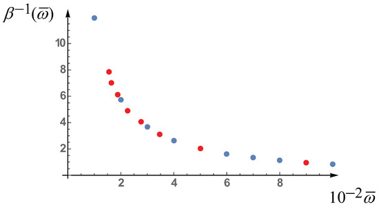
Figure 1.
The dependence of a quantity on the dimensionless frequency. As calculations show, in the frequency range under consideration (see table) there are only eight values of (red points), for which the quantization conditions (45) and (46) are satisfied. The blue dots denote such states for which the quantization conditions are not satisfied.
Now we consider the problem of localization of the solution . Taking into account the fact that , the Equation (42) can be written in the form:
In particular, as follows from the Equation (47), all solutions (44) are localized on the manifold (one-quarter of the plane , where the bracket denotes the entire plane (see Figure 2).
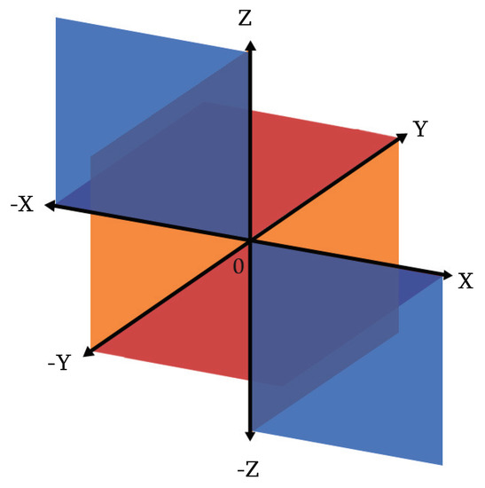
Figure 2.
The coordinate system divides the three-dimensional space into eight spatial regions using three planes. The boson of a vector field (hion) with projection of spin +1 is a two-dimensional structure consisting of six components localized on the following manifolds and , respectively.
The imaginary part of the wave function is calculated similarly and has the same form, but in this case the solution must satisfy the following trigonometric equation:
Obviously, the Equation (48) defines another quarter of the plane , on which the solution is localized. As for the wave function , then it is localized on the manifold .
A similar investigation for the projections of the wave function and shows that the separation of variables in corresponding equations is possible taking into account the following algebraic equations:
Analysis of the Equation (49) shows that the projections of the wave function are localized on the following manifolds; and .
Thus, we have proved the possibility of the formation of a stable massless Bose particle with spin 1–hion as a result of random fluctuations of the QVF. As can be seen the obtained solutions (44) combine the properties of quantum mechanics and the theory of relativity and, respectively, maximally reflect to the ideas of string theory. It is interesting to note that the ground state of the vector boson characterized the highest frequency.
4. Quantum Distribution in Different Hion States
Let us consider the solution of the Equation (43) in the ground state.
Taking into account (39) and (44), we can get the following solution:
where
in addition, the indices of the wave function denote the quantum numbers , accordingly, the constant C is defined below from the normalization condition of the wave function, in addition, is the characteristic spatial dimension of the vector boson in the ground state, which can be calculated taking into account the Equations (29) and (34):
Recall that in (51) the frequency , where dimensionless frequency of the ground state is equal (see Table 1 and Figure 1). In the framework of the developed approach, it is impossible to determine the constant , since the speed c and fluctuations power remain free parameters of the theory. Apparently, these parameters will have to be refined experimentally and introduced into the theory as fundamental constants.

Table 1.
The average-statistical dimensionless frequency of the system in different quantum states (see condition (45)).
As for the wave function , it is also described by the expressions (50), but with the only difference that in this case the wave function is localized on the manifold . In a similar way one can obtain solutions for the wave functions and localized on the corresponding manifold.
Now we can write down the normalization condition for the full wave function:
where .
Considering that the projections of the full wave function are localized on different non-intersecting manifolds and the definition (52), we can write:
Below as an example, we will calculate the first term of the integral, considering the case of the ground state. Taking into account that the wave function can be represented in the form , we can write:
where denotes radius-vector r on the plane , in addition, in calculating the integral, we assume that the wave function in the direction x perpendicular to the plane is the Dirac delta function.
Considering (53) and (54), we can determine the normalization constant of the wave function (50), which is equal to . Note that in a similar way one can obtain the hion wave function with the spin projection –1 (see Appendix B).
Now we can calculate the probability distribution of the hion’s x-projection in the ground state. Using (50), we obtain the following expression for the probability distribution on the surface element :
where and .
Recall that the angle coincides with the angle on the fixed plane.
Integrating the expression (55) by the angle , we obtain the probability distribution of the ground state depending on radius:
Finally, calculating the expression (56), we find that for the value and, respectively, for , the probability distribution has a maximum (see Figure 3).
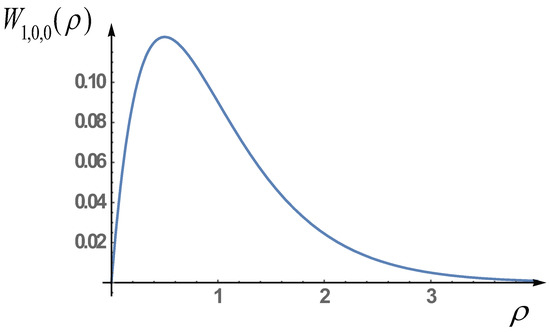
Figure 3.
The probability distribution of hion in the ground state depending on the radius. The distance , or more precisely , at which the maximum value of the amplitude of the hion probability is reached.
Now we consider the first three excited quantum states, which are characterized by the principal quantum number . Using the solution (44), we can write the explicit form of these wave functions:
where
Taking into account expressions (57), we can construct a radial probability distribution for the first four excited states of the hion:
Recall that at deriving of expressions for the probability distributions , and , averaging over the angle is performed. Note that the probability distributions (see Figure 4), and also the energies of considered three states coincide. In particular, the quantum state described by the wave function has the energy , whereas three different quantum states , and are characterized by the same energy .
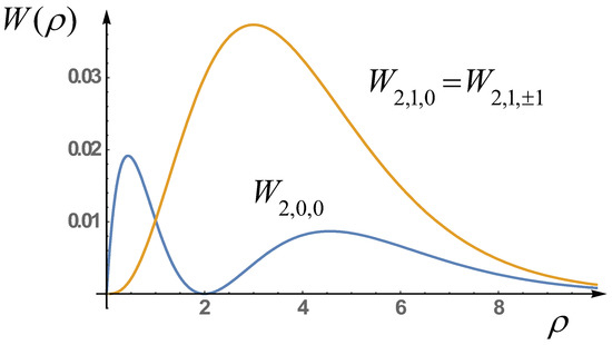
Figure 4.
The probability distributions of the first four excited states of the hion depending on radius. The orange curve in the graph shows the probability distributions in various three excited states.
5. The State of the Hion on the Next Scale of Relaxation
So far we have investigated the possibility of the formation of hion as a result of the continuously fluctuations of QVF on the first phase of relaxation, while such phases can be a few. In this connection, the natural question arises: namely, how the state of the hion changes if we take into account random fluctuations of QVF of the next order, i.e., consider the change of the particle on the next evolutionary scale .
Let us consider the evolution of hion with the spin projection +1 taking into account the influence of the random environment in the framework of SDE of the type:
and also the equation:
where denotes the generator of random forces, and is the 4D-interval in which these random influences are carried. The Equation (58) can be represented in matrix form:
and the Equation (59), respectively, in the form:
For further constructions, the system of Equations (60) and (61) must be reduced to the canonical form:
where and , in addition:
For simplicity, we will use a random generator that satisfies the conditions of white noise:
where and in addition, it is assumed that the bracket means averaging over the relaxation time .
The joint probability distribution of QVF can be represented in the form (see [33]):
where the set of wave functions denotes vacuum fields, and . In addition, in (65) the function denotes the Dirac delta function in the three-dimensional Hilbert space, in addition, by default we will assume that the wave function is dimensionless, i.e., it is multiplied by a constant value (see (50)).
Now using the system of SDE (62)–(64), for the conditional probability (65) the following second order partial differential equation can be obtained [33]:
where denotes the complex conjugate of the wave function and , which is a dimensionless quantity denoting the fluctuations power. In the equation (66) the following notations also are made; and .
The general solution of the Equation (66) is convenient to represent in the integral form:
where and the function denotes the initial condition of the Equation (66) at , before switching on the interaction with the random environment. Since before switching on the interaction, the hion (the vector-boson) is in a pure quantum state, i.e., in the Hilbert space is determined by a fixed vector , then we can put; , where has the sense of the distribution hion, which is defined as follows:
where
Substituting the expressions (68) and (69) into (67) and integrating over the variables within , we obtain the expression for the deformation of the initial quantum distribution , taking into account the evolution of a hion in a random environment:
where
Note that the function characterizes the deformation of the initial distribution:
Integrating (67) taking into account (70) and (71), we obtain the quantum distribution of a hion with consideration of the random influence of an environment. It is easy to see that before the relaxation, the 4D-interval is zero, i.e., and, accordingly, the deformation coefficient , as expected.
By similar reasoning, we can calculate the deformation of the hion state vector:
Thus, it is obvious that the deformation of the quantum state hion leads to a breaking of symmetry, which leads to spontaneous transitions from ground state to another, massless, and also mass states.
It is important to note that despite the fact that the hion is deformed under the influence of random influences of the environment, nevertheless the full probability is conserved. In particular, if to integrate the representation (67) over the fields , then, obviously, we can get:
where .
Recall that integration over the Hilbert space is equivalent to integration over the configuration space . This is an obvious proof that the probability is preserved.
6. Formation of Singlet and Triplet Pairs of Hions
At the second stage of relaxation in the ensemble hions, the formation of singlet and triplet states are possible by entangling them [41].
As it is well known [42], there are four possible entangled states of the so-called Bell states, which can be represented as:
where the radius vectors and determine positions of the first and second hions, respectively. Note that the first equation denotes possible two singlet states, and the second two triplet states. In (73) the following notations are also made:
where we recall that the wave functions and denote the pure states of hions with the spin projections +1 and –1, respectively. In (73) the dash over a wave function denotes complex conjugation, denotes the transposed vector and the symbol ⊗, respectively, denotes the tensor product between the vectors.
The explicit form of a direct tensor product between vectors with opposite spins have the following form:
whereas the direct tensor product between vectors with parallel spins can be represented as:
where and denote the third-rank matrices, while and are their complex conjugate matrices.
6.1. The Zero-Spin Particles and the Scalar Field
Now the main question is the question of the so-called quintessence- is it possible to form particle-like excitations in the form of some dynamic scalar field [14]?
Using the first equation of the system (73), we can construct the boson wave function with zero spin, entangling two hions with opposite spin projections, presenting it in the form (see Appendix B):
where the matrix elements are calculated explicitly. Taking into account the rule of localization of the wave function components on the corresponding planes (see Figure 2), we obtain:
Note that the matrix elements with the plus sign are zero , since it is possible easy to show that the components of the corresponding wave functions are localized on disjoint manifolds. Latter means that the wave state does not exist. In other words, in the case of the Minkowski space–time there is only one singlet state for zero-spin boson.
The quantum distribution of the scalar boson in the singlet state before the onset of the relaxation process, i.e., for , can be represented as:
where
is a diagonal third rank matrix, the elements of which have the following form:
Taking into account the fact that the spins of two vector states and are directed oppositely, and also considering features of spatial localization these quasi-particles, we obtain the following expressions for the matrix elements:
Now let us consider how the density of the quantum distribution of a scalar boson changes taking into account the random influence of the environment.
To study this problem, we will use the following system of complex stochastic matrix equations:
and also the equations:
where denotes the radius-vector of corresponding hion, in addition, the complex generators describing random fluctuations of charges and currents, which continuously arise in 4D-interval .
For further studies, the system of Equation (82), it is useful to write in the matrix form:
and, respectively,
where and
As in the case of one hion (see (62) and (63)), the system of SDE (84) can be reduced to the canonical form:
where and , in addition, the following notations are made:
Below in the Equations (85) and (86), we will assumed that the following relations are satisfied:
which is quite natural.
As in the case of a single hion, we will assume that the random generator satisfies the correlation properties of white noise (see Equations (64)).
The joint probability distribution for a scalar boson can be represented as (see [33]):
where denotes a set of fluctuating vacuum fields and . In the representation (87) the function denotes the Dirac delta function generalized on a 6D-Hilbert space.
Using the SDE system (85), for the conditional probability describing the relaxation of the singlet state, we can obtain the following partial differential equation of the second order (see [33]):
where denotes the complex conjugate of the function and .
For further analytical calculations, it is convenient to represent the general solution of the equation (88) in the integral form:
where , in addition, as in the case of a single hion, we assume that is the initial distribution of the scalar boson before the relaxation begins. It is obvious that integration over the space–time, i.e., by the spectrum, in accordance with the ergodic hypothesis, is equivalent to integration over the full 12D space.
Recall that denotes the mean value:
where
in addition, performing similar calculations, as in the case of a single hion (see (67)–(71)), we can get:
Note that, using analogous arguments, we can construct the wave function of two entangled hions with consideration of its relaxation in a random environment. Also, performing calculations similarly to the case of one hion, one can see that the deformation of the wave state of one scalar boson under the influence of a random environment does not lead to a violation of the law of conservation of full probability.
Thus, we have shown that, as a result of the multi-scale evolution of QVF, a scalar field is formed, as a sort of Bose-Einstein condensate of massless scalar bosons. However, such a condensate differs significantly from a conventional substance, since it consists of massless particles that have a large Compton wavelength that can not thicken unlimitedly and to form large-scale structures such as stars, planets, etc. In other words, the described substance meets all the characteristics of the quintessence requirements and, accordingly, it can be asserted that the quintessence hypothesis is theoretically proved.
6.2. Triplet State of Two Hions and the Vector Field
The wave function of the triplet state formed by entangling two hions with parallel projections of the spin can be represented as:
where, as shown by simple calculations, the following equalities hold:
From these equalities it follows that there is only one triplet state, which described by the matrix of the third rank .
The relaxation of the triplet state (92) can be taken into account using a similar construction, as in the case of the singlet state (89). In this case, however, the following substitutions must be made in the expressions (85) and (86), which will be equivalent to transforming the singlet state into the triplet state. Note that these replacements in the expression (89) changes the power of fluctuations .
7. Conclusions
Although a fundamental scalar field has not yet been observed experimentally, it is generally accepted that such fields play a key role in the construction of modern theoretical physics of elementary particles. There are a few important hypothetical scalar fields, for example the Higgs field for the Standard Model, the dark energy–quintessence for a theory of the quantum vacuum, etc. Note that the presence of each of them is necessary for the complete classification of the theory of fundamental fields, including new physical theories, such as, for example, String Theory. Recall that despite the great progress in the representations of modern particle theory within the framework of the SM, it does not give a clear explanation of a number of fundamental questions of the modern physics, such as “What is dark energy and dark matter?” or “What happened to the antimatter after the big bang?” and so on. As modern astrophysical observations show, not less than 74 percent of the energy of the universe is associated with a substance called dark energy, which has no mass and whose properties are not sufficiently studied and understood. Based on many considerations, it was obvious to assume that this substance must be related to a quantum vacuum or simply be QV itself.
As it is known, in the modern understanding of what is called the vacuum state or the quantum vacuum, it is by no means a simple empty space. Recall that in the vacuum state, electromagnetic waves and particles continuously appear and disappear, so that on the average their value is zero. It would be reasonable to think that these fluctuating or flickering fields are born as a result of spontaneous decays of quasi-stable scalar massless particles, very inert to any external influences.
The main purpose of this work was the theoretical justification for the possibility of forming a scalar field consisting of uncharged massless zero-spin particles. The developed approach is formally similar to the Parisi–Wu [30,43] stochastic quantization, however it also has significant differences. In particular, as in the case of the Parisi–Wu stochastic quantization, when considering Euclidean quantum field theory, we consider the stochastic Yang–Mills equations as the basic equations. However, unlike the Parisi–Wu concept, we believe that the nature of stochasticity is multi-scale and, therefore, the equilibrium limit of the statistical system associated with a heat reservoir is not one, but many. In other words, there are many quasi-equilibrium states between which spontaneous transitions occur, but at the same time the dynamical equilibrium between these states is conserved. Another significant difference between the developed representation and the Parisi–Wu theory is that the analogy with classical statistical physics is not used for determination the stationary distribution of a random process. The latter circumstance allows us to avoid a number of inaccuracies inherent in standard representations, which, in our opinion, makes it difficult to study such a specific substance as QV.
In this article, we have considered the simplest case when the self-action terms are absent in the Yang–Mills stochastic equations, that is, . This means that considered QVF are Abelian fields, which satisfy the gauge group symmetry . We quantized the classical stochastic vector field (see quantization conditions (46)) and proved that on the main relaxation scale , in the Hilbert space, in the limit of statistical equilibrium, a discrete set of stationary solutions (44) arises, describing a massless spin-1 Bose particle (named hion). It is important to note that these solutions, combining relativism with quantum mechanics together (see Equation (22)), are as close as possible to the concept of 2D quantum string theory. It is shown that hion is characterized by three quantum numbers, where the ground state is characterized by the highest frequency. As shown in our study, the hion in the space is localized on the complex 2D surface consisting of three perpendicular planes (see Figure 2).
We have proved that on the second scale of relaxation , hion becomes quasi-particle, which can make spontaneous transitions to other mass and massless states. Note that during spontaneous transitions hion the bosons and B combine into two different bosons, such as the photon (electromagnetic interaction) and the massive boson (weak interaction). It is also shown that on the second relaxation scale, two hions with spin projections +1 and −1 can form a boson with zero spin. The ensemble of spin-0 bosons forms a Bose-Einstein condensate, which is a scalar field with all the necessary properties. In other words, the work is a theoretical proof of the dark energy–quintessence hypothesis and, accordingly, the stability of the QED vacuum in the infrared limit. Recall that in the infrared limit of vacuum diagrams does not exist in theories with self-interacting massless fields (QCD) or massless interacting particles (massless QED), if the theory is renormalizable [16,17].
Note that a small part of the energy of a quantum vacuum is concentrated in vector fields consisting of hions and vector bosons with spin 2. These fields on a large scales of space can be represented as Heisenberg spin glass, the total polarization of which is zero.
A very important question related to the value of the parameter (see (51)), which characterizes the spatial size of the hion, remains open within the framework of the developed representation. Apparently, we can get a clear answer to this question by conducting a series of experiments. In particular, if the value of the constant will be substantially different from the Planck length , then it will be necessary to introduce a new fundamental constant defining the spatial size of the hion. We are convinced that if it will be impossible to conduct direct measurements of constants , characterizing the fluctuations of quintessence, and, accordingly, formation of hions, then this can be done using of indirect measurements. In particular, we believe that interesting experiments on the detection of optical force between controlled light waves, known as “optical binding strength” (see for example [44]), are not related to the Casimir vacuum properties, as some researchers are trying to explain. The magnitude of the optical force and its diverse behavior do not allow us to hope for it. To explain these forces, most likely, there must be a more “fundamental vacuum” with more non-trivial properties like as scalar field or dark energy. A different experiments aimed at non-invasive measurements of various characteristics of biological organisms and systems with fluctuating entropies also push us to the idea of the existence of quintessence, with its still unknown properties [12].
Thus, studies carried out within the framework of the symmetry group allow us to speak of the properties of the QVF and, accordingly, of the structure and properties of empty space–time down to the distances m, when strong interactions begin to dominate. As preliminary studies show, the properties of space–time can change as a result of the polarization of the vector component QV and, accordingly, changes in the refractive indices of the vacuum due to orientational effects of hions in external, even weak electromagnetic fields. Obviously, in this case the photon-photon interaction and, accordingly, the interaction of two light beams occurs according to another physical mechanism, which differs from the mechanism described by the fourth-order Feynman diagrams. In other words, there is every reason to speak for the first time about the real, rather than theoretical, possibility of implementing space–time engineering.
It is also important to note that the developed theory on the second relaxation scale allows us to derive a second-order partial differential equation that takes into account the mutual influence of isospins with an arbitrary constant . In addition, the new concept can be easily generalized to the case of others symmetries, which is extremely important for a more complete understanding of the properties and structure of dark energy–quintessence.
Finally, as many researchers point out, beginning of the middle of the twentieth century a new scientific–technological revolution began, based not on energy but on information. In this regard, some researcher are rightly identified the Universe with giant quantum computer, which can explain previously unexplained features, most importantly, the co-existence in the universe of randomness and order, and of simplicity and complexity (see, for example [45]). In the light of the above theoretical proofs, the quantum vacuum–quintessence or scalar field is nothing more than a natural quantum computer with complex logic, different from that currently being realized in practice.
Funding
This research received no external funding.
Conflicts of Interest
The author declare no conflict of interest.
Appendix A
Let us consider the limit of statistical equilibrium . In this case, the partial differential Equation (31) is transformed into the ordinary differential equation of the form:
Proposition A1.
We represent the solution of the Equation (A1) in the form:
Let the function satisfies the equation:
then it will look like:
where is the arbitrary constant.
If we choose then the function will be positive on all axis .
Substituting (A3) into (A1), we get:
where
As follows from the analysis of the coefficient , on the axis , it has types of uncertainties or . Applying the L’Hôpital’s rule, for the coefficient near the critical points , where uncertainties appear, we obtain the expression:
In asymptotic domains, i.e., when in the Equation (A7), we can neglect the term and to obtain the following solution:
whereas the asymptotic solution of the Equation (A1), respectively, is:
Again using the L’Hôpital’s rule, it can be proved that:
from which flow out the estimation:
and, respectively;
Now let us represent the integral (A2) in the form of a sum from three terms:
where
For the first and third integrals, we can write down the following obvious estimates (see (28)):
and, respectively:
As for the second term in (A11):
then it is obviously converges , since the function is bounded, and the integration is performed on a finite interval.
Appendix B
Using the systems of Equations (15)–(11) and carrying out a similar calculations for vacuum fields consisting of particles with projections of spin -1, we can obtain the following system of equations:
In (A15) substituting the solutions of the equations in the form:
we obtain the following system of stationary equations:
Further, carrying out standard arguments, we find the following stationary equations:
The solution of the system of equations is conducted in a similar way, as for fields (see Equations (32)–(35)). In particular, calculations show that the components of the vector boson with the spin –1 projection are localized on a manifold consisting of the following set of planes; and , respectively.
References
- Saunders, S.; Brown, H.R. (Eds.) The Philosophy of Vacuum; Oxford University Press: Oxford, UK, 1991. [Google Scholar]
- Lamb, W.E., Jr.; Retherford, R.C. Fine Structure of the Hydrogen Atom by a Microwave Method. Phys. Rev. 1947, 72, 241. [Google Scholar] [CrossRef]
- Casimir, H.B.G. On the attraction between two perfectly conducting plates. Proc. R. Neth. Acad. Arts Sci. 1948, 51, 793–795. [Google Scholar]
- Fulling, S.A. Nonuniqueness of Canonical Field Quantization in Riemannian Space-Time. Phys. Rev. D 1973, 7, 2850. [Google Scholar] [CrossRef]
- Schwinger, J. On Quantum-Electrodynamics and the Magnetic Moment of the Electron. Phys. Rev. 1948, 73, 416. [Google Scholar] [CrossRef]
- Langbein, D. Theory of van der Waals Attraction; Springer Tracts in Modern Physics; Springer: Berlin/Heidelberg, Germany, 1974. [Google Scholar]
- Burke, D.L.; Field, R.C.; Horton-Smith, G.; Spencer, J.E.; Walz, D.; Berridge, S.C.; Bugg, W.M.; Shmakov, K.; Weidemann, A.W.; Bula, C.; et al. Positron Production in Multiphoton Light-by-Light Scattering. Phys. Rev. Lett. 1997, 79, 1626. [Google Scholar] [CrossRef]
- Hawking, S. A Brief History of Time; Bantam Books: New York, NY, USA, 1988. [Google Scholar]
- Gurzadyan, V.G.; Xue, S.-S. On the estimation of the current value of the cosmological constant. Mod. Phys. Let. A 2003, 18, 561. [Google Scholar] [CrossRef]
- Weinberg, S. The Cosmological Constant Problems. arXiv 2000, arXiv:astro-ph/0005265v1. [Google Scholar]
- Gevorkyan, A.S.; Gevorkyan, A.A. Maxwell Electrodynamics Subjected to Quantum Vacuum Fluctuations. Phys. Atom. Nucl. 2011, 74, 901–907. [Google Scholar] [CrossRef]
- Sargsyan, R.S.; Karamyan, G.G.; Gevorkyan, A.S. Quantum-mechanical channel of interactions between macroscopic systems. AIP Conf. Proc. 2010, N1232, 267–274. [Google Scholar]
- Gevorkyan, A.S. Quantum Vacuum and Structure of Empty Space-Time. Phys. Atom. Nucl. 2018, 81, 809–818. [Google Scholar] [CrossRef]
- Caldwell, R.R.; Steinhardt, P.J. Imprint of gravitational waves in models dominated by a dynamical cosmic scalar field. Phys. Rev. D 1998, 57, 6057. [Google Scholar] [CrossRef]
- Novikov, E.A. Ultralight gravitons with tiny electric dipole moment are seeping from the vacuum. Mod. Phys. Lett. A 2016, 31, 1650092. [Google Scholar] [CrossRef]
- Savvidy, G.K. Infrared instability of the vacuum state of gauge theories and asymptotic freedom. Phys. Lett. B 1977, 71, 133–134. [Google Scholar] [CrossRef]
- Scharf, G. Vacuum stability in quantum field theory. Il Nuovo Cim. A 1996, 109, 1605–1607. [Google Scholar] [CrossRef]
- Higgs, P.W. Broken symmetries and masses of gauge bosons. Phys. Rev. Lett. 1964, 13, 508. [Google Scholar] [CrossRef]
- Higgs, P.W. Broken symmetries, massless particles and gauge fields. Phys. Lett. 1964, 12, 132. [Google Scholar] [CrossRef]
- Oppenheimer, J.R. Note on light quanta and the electromagnetic field. Phys. Rev. 1931, 38, 725. [Google Scholar] [CrossRef]
- Molière, G. Laufende elektromagnetische Multipolwellen und eine neue Methode der Feld-Quantisierung. Annalen der Physik 1949, 6, 146. [Google Scholar] [CrossRef]
- Weinberg, S. Feynman rules for any spins. II Massless particles. Phys. Rev. 1964, 134, 882–896. [Google Scholar] [CrossRef]
- Wolf, E. (Ed.) Progress in Optics; Elsevier: Amsterdam, The Netherlands, 1996; Volume XXXVI, Chapter 5; pp. 245–294. [Google Scholar]
- Gell-Mann, M. A Schematic Model of Baryons and Mesons. Phys. Lett. 1964, 8, 214–215. [Google Scholar] [CrossRef]
- Silberstein, L. Elektromagnetische Grundgleichungen in bivectorieller Behandlung. Annalen der Physik 1907, 327, 579–586. [Google Scholar] [CrossRef]
- Yang, C.N.; Mills, R. Conservation of Isotopic Spin and Isotopic Gauge Invariance. Phys. Rev. 1954, 96, 191–195. [Google Scholar] [CrossRef]
- Caprini, I.; Colangelo, G.; Leutwyler, H. Mass and width of the lowest resonance in QCD. Phys. Rev. Lett. 2006, 96, 132001. [Google Scholar] [CrossRef] [PubMed]
- Clay Mathematics Institute. Available online: http://www.claymath.org/millennium-problems/yang-mills-and-mass-gap (accessed on 26 September 2018).
- Biro, T.S.; Matinyan, S.G.; Muller, B. Chaos and Gauge Field Theory; World Scientific Lecture Notes in Physics; World Scientific: Singapore, 1995. [Google Scholar]
- Damgaard, P.H.; Hüffel, H. Stochastic quantization. Phys. Rep. 1987, 152, 227–398. [Google Scholar] [CrossRef]
- Faddeev, L.D.; Popov, V.N. Feynman diagrams for the Yang-Mills field. Phys. Lett. B 1967, 25, 29. [Google Scholar] [CrossRef]
- Faizal, M.; Momeni, D. Universality of Short Distance Corrections to Quantum Optics. Available online: http://arxiv.org/abs/1811.01934v1 (accessed on 16 December 2013).
- Gevorkyan, A.S. Nonrelativistic quantum mechanics with fundamental environment. In Theoretical Concepts of Quantum Mechanics; Pahlavani, M.R., Ed.; InTech: Rijeka, Croatia, 2012; Chapter 8; pp. 161–186. ISBN 978-953-51-0088-1. [Google Scholar]
- Klyatskin, V.I. Statistical Description of Dynamical Systems with Fluctuating Parameters; Nauka: Moscow, Russia, 1975. (In Russian) [Google Scholar]
- Lifshits, I.M.; Gredeskul, S.; Pastur, L. Introduction to the Theory of Disordered Systems; Wiley-VCH: Hoboken, NJ, USA, 1988; 462p. [Google Scholar]
- Frisch, H.L.; Lloyd, S.P. Electron Levels in a One-Dimensional Random Lattice. Phys. Rev. 1960, 120, 1175. [Google Scholar] [CrossRef]
- Von Neumann, J.V. Proof of the quasi-ergodic hypothesis. Proc. Natl. Acad. Sci. USA 1932, 18, 70–82. [Google Scholar] [CrossRef] [PubMed]
- Birkhoff, G.D. Proof of the ergodic theorem. Proc. Natl. Acad. Sci. USA 1931, 17, 656–660. [Google Scholar] [CrossRef]
- Landau, L.D.; Lifshitz, L.M. Quantum Mechanics. In Non-Relativistic Theory, 3rd ed.; Elsiever Science LTD: Amsterdam, The Netherlands, 2004. [Google Scholar]
- Abramowitz, M.; Stegun, I.A. (Eds.) Orthogonal Polynomials. In Handbook of Mathematical Functions with Formulas, Graphs, and Mathematical Tables, 9th ed.; Dover: New York, NY, USA, 1972; Chapter 22; pp. 771–802. [Google Scholar]
- Einstein, A.; Podolsky, B.; Rosen, N. Can Quantum-Mechanical Description of Physical Reality Be Considered Complete? Phys. Rev. 1935, 47, 777. [Google Scholar] [CrossRef]
- Whitaker, A. John Stewart Bell and Twentieth-Century Physics: Vision and Integrity; Oxford University Press: Oxford, UK, 2016; Chapter 2. [Google Scholar]
- Parisi, G.; Wu, Y.-S. Perturbation Theory without Gauge Fixing. Sci. Sin. 1981, 24, 483. [Google Scholar]
- Li, M.; Pernice, W.H.P.; Tang, H.X. Tunable bipolar optical interactions between guided lightwaves. Nat. Photonics 2009, 3, 464–468. [Google Scholar] [CrossRef]
- Lloyd, S. The Universe as Quantum Computer. Available online: http://arxiv.org/abs/1312.4455v1 (accessed on 16 December 2013).


© 2019 by the author. Licensee MDPI, Basel, Switzerland. This article is an open access article distributed under the terms and conditions of the Creative Commons Attribution (CC BY) license (http://creativecommons.org/licenses/by/4.0/).