Article

Power-Based Statistical Detection of Substance Accumulation in Constrained Places Using a Contact-Less Passive Magnetoelastic Sensor

by
Ioannis Kalyvas
and
Dimitrios Dimogianopoulos
*
Department of Industrial Design and Production Engineering, University of West Attica, 12241 Athens, Greece
*
Author to whom correspondence should be addressed.
Vibration 2025, 8(4), 64; https://doi.org/10.3390/vibration8040064
Submission received: 21 July 2025 / Revised: 25 September 2025 / Accepted: 6 October 2025 / Published: 10 October 2025

Abstract

A contactless passive magnetoelastic sensing setup, recently proposed for detecting pest/substance accumulation in confined spaces (labs, museum reserves), is optimized for enhanced low-frequency performance. The setup uses a short flexible polymer slab, clamped at one end. There, a short Metglas® 2826MB magnetoelastic ribbon is fixed upon the slab’s surface. The opposite end receives excitation by a remotely controlled module of ultra-low amplitude vibration. When vibrating (with the slab), the ribbon generates magnetic flux, which depends on (and reflects) the slab’s dynamics. This changes when loads accumulate on its surface. The flux induces voltage in a contactless manner in a low-cost pick-up coil suspended above the ribbon. Voltage monitoring allows for evaluation of the vibrating slab’s real-time dynamics and, consequently, the detection of load-induced changes. This work innovates by introducing a low-cost passive circuit for real-time voltage processing, thus achieving an accurate representation of the low-frequency dynamics of the magnetic flux. Furthermore, it introduces an algorithm, which statistically detects load-induced changes using the voltage’s low-frequency power characteristics. Both additions enable load detection at relatively low frequencies, thus addressing a principal issue of passive contactless sensing setups. Extensive testing at different occasions demonstrates promising load detection performance under various conditions, especially given its cost-efficient hardware and operation.

1. Introduction

A critical application of remotely controlled sensing devices regards their use in places of difficult and/or dangerous access without proper personal protection. Obviously, such places include (industrial or research) lab facilities where chemical, microbiological, or similarly hazardous agents may accumulate during their operation. However, sites such as collection reserves of (small) museums or facilities used for storing objects of cultural heritage also have constrained access, usually on a need-to-do basis, for technical staff [1,2,3], while facing a similar problem of destructive (to stored objects) substances/agents like pests, accumulating on site. In this case, an additional issue is that the resources for investing in state-of-the-art remotely controlled sensors are limited, unlike, for instance, large industrial sites where funding is less of a problem. In all cases, technologies for remotely detecting critical substances or agents accumulating in a monitored site are vital, so that technical staff may intervene only when absolutely needed.
Magnetoelasticity, also referred to as magnetostriction, is a property exhibited by some (ferromagnetic) materials, whereby their shape is modified due to external varying magnetic fields. They may also produce magnetic flux if subjected to external variable excitation [4,5,6], due to mechanical or electromagnetic sources. An interesting class of applications involves magnetoelastic ribbons of short length, clamped on both sides and placed inside a given environment. Imposing an external varying magnetic field causes the ribbon to experience small but alternating longitudinal changes. Since clamped on both sides, the ribbon will experience vibration, with dynamics related to the variability (pattern and magnitude) of the external magnetic field and, critically, its dimensions and mass distribution. Hence, if biological agents [7,8], air pollutants [9], volatile organic compounds [10], H2O [11,12,13], or H2O2 [14] start accumulating on the ribbon’s surface at a given moment, its mass distribution will change. This will be the only cause of altered dynamics of the vibrating ribbon, if the external magnetic excitation remains unchanged. Then, remote monitoring of the vibrating ribbon’s dynamics allows for detecting accumulation of substances on its surface, and consequently in its environment.
Various different remote detection setups use this principle of operation. The magnetoelastic ribbon (or other element) is often designed to vibrate at its resonant frequency by means of an interrogation coil, suitably driven by electrical current, to provide a variable magnetic flux without bearing contact with the ribbon. Then, a second (pick-up) coil suspended above the ribbon (again bearing no contact with it) receives the magnetic flux emitted from the vibrating ribbon and generates voltage. The latter can be uploaded to a remote host, so that any frequency shifts pointing to substance accumulation may be detected. This technical approach involving a pick-up coil and an interrogation coil is referred to as the active design [15] and is quite sensitive to detecting mass accumulation on the ribbon surface, with examples found in [7,8,9,10,11,12,13,14]. Detection sensitivity and the quality factor (effectively the sharpness of sensor resonance) of active setups have been extensively studied (in [8], for instance) both experimentally and theoretically. Numerous efforts to optimize the magnetic signal generated have been noted, either by selecting a magnetoelastic ribbon based on Young’s modulus and ∆E effect characteristics [16] or by studying its length-to-width ratio [16,17,18], or even its shape, with hour-glass [19] or rhomboid forms [20,21] considered more effective. Such efforts have been extensively presented in [22]. Lastly, apart from suitably selecting or shaping the magnetoelastic material, other efforts to optimize the magnetic signal emitted focus on its thermal processing (annealing) [23].
As previously stated, the magnetoelastic ribbon must receive excitation in order to vibrate and generate magnetic flux, subsequently used for detection purposes. External excitation may also be provided by mechanical devices, structures and, in general, machinery with reciprocating parts. The main difference from the previous case is that now the ribbon vibrates in accordance with the devices or structures upon which it is mounted. Consequently, the ribbon sets into vibration without requiring an interrogation coil and generates magnetic flux proportionally to the vibrating characteristics of its mounting basis (instead of its own shape and dimensions). This approach is referred to as the passive setup [15], and the main difference from the active one is the absence of an interrogation coil (and of the associated requirements for its electrical feed and circuitry). Hence, analyzing the spectral characteristics of the recorded voltage (generated via a pick-up coil suspended above the ribbon) allows for detecting frequency shifts either from mass accumulation on the ribbon’s mounting surface [24,25], from changing frequency levels of mechanical excitation [25], or even from structural faults affecting the structure/device upon which the ribbon is mounted [26,27,28,29,30,31]. Thus, the passive setup is appropriate for fault detection and isolation (FDI) tasks in structures and/or systems. Due to the lack of an interrogation coil and the associated electrical or electronic circuits, passive setups have lower operational costs and are far simpler in terms of the hardware used. However, their main weakness is that, even when using a high-performance coil, the generated magnetic flux is significantly weaker than that obtained by active setups. As a remedy to this problem, sometimes a second coil fed by a simple DC-circuit is employed for biasing the magnetic flux produced and yielding better results [31,32]. Nonetheless, biased or not, the signals obtained by passive setups are, in general, noisy with signal dynamics hidden by noise, especially at low frequencies. This issue is avoided by focusing on relatively higher frequencies and, especially, by carefully designing the algorithm detecting changes in the recorded signal’s spectral characteristics and, hence, faults/failures in the underlying structure or machinery [26,27,28].
The current work considers the passive setup proposed in [24,33] and innovates by redesigning the signal acquisition process and algorithmic analysis, in an effort to achieve comparable detection results to those in [33], but at lower frequencies and without the influence of high-frequency noise. Indirectly, the current proof-of-concept work demonstrates that detection is possible in low frequencies even with noisy/weak signals (such as those generated by passive setups). Briefly, a thin and flexible polymer slab is secured as cantilever, with a short Metglas® 2826MB magnetoelastic ribbon fixed on the surface of its clamped end. A remotely controlled module of vibration supplies ultra-low amplitude vibration to the opposite end. When vibrating with the slab, the ribbon generates magnetic flux, which in turn induces voltage in a pick-up coil suspended above the ribbon. The voltage is, now, recorded via a specific passive circuit, designed for accurately representing the low-frequency dynamics (above 0.48 Hz) of the emitted magnetic flux. In conjunction with the use of a novel algorithm based on the power of recorded (and processed) signals, it is now possible to detect spectral changes in the recorded data induced by light loads (pest) accumulating on the slab at frequencies from 200 Hz onward. Hence, any potential influence of transient high-frequency noise can be avoided, yielding a more robust detection setup with respect to noise. The current passive setup, hence, alleviates the main drawback of reduced detection performance in the presence of noisy signals. On the other hand, it retains the advantages of simplicity and low hardware and operating costs (due to the absence of interrogation coils as in [7,8,9,10,11,12,13,14]). Extensive testing that took place on three different occasions (and underlying noise conditions), demonstrates promising load-detection performances at all times, especially given its cost-efficient operation and hardware. The paper is organized as follows: After a comprehensive introduction in Section 1, the setup is presented in Section 2, both in terms of hardware and algorithmic design. Section 3 presents the results of testing, whereas Section 4 provides an extensive discussion on the findings of Section 3. Finally, Section 5 presents some concluding remarks.

2. Materials and Methods

2.1. The Hardware Components of the Setup

The experimental setup is presented in Figure 1 and is principally based on that proposed in [33]. The hardware components involve the following:
  • A flexible polymer slab measuring 100 mm × 30 mm × 0.8 mm with a Metglas® 2826MB ribbon (METGLAS® Inc., Conway, SC, USA) of 25 mm × 5 mm. The ribbon is laterally centered on the slab surface and fixed with cyano-acrylic glue (see Figure 1b).
  • A vice used for clamping the slab’s end where the ribbon is fixed upon. The opposite end is free and flexes due to its own weight (unless supported, see Figure 1b).
  • The support of the free end, which also provides excitation. In [33], a feature phone was used to support the free end and provide excitation via its vibrating mode. Here, a suitably mounted low-cost vibration module similar to those found in cellular phones is used. The DC-vibrator, as will be referred to hereafter, provides excitation to the slab via a (battery fed) Arduino® Uno microcontroller (Arduino®, Monza, Italy) remotely connected to (and driven by) a personal computer.
  • A low-cost pick-up coil Vishay IWAS-3827EC-50 (Vishay Intertechnology, Inc., Malvern, PA, USA) placed 15 mm above the ribbon, with this value resulting from an optimization experiment in [33]. Hence, the magnetic flux produced by the vibrating group of slab and ribbon induces voltage into the pick-up coil in a contactless manner. This voltage is fed to a resistor–capacitor (RC) circuit shown in Figure 1a,c. The RC-circuit design is presented in Section 2.2.
  • A load of 0.46 g simulated by six needles stuck together and secured via thin adhesive strips at the W4 position (Figure 1b). This was the lowest detectable value of load in [24,33] and is thus used here as a basis for assessing results with respect to [33]. Position W4 is 4 cm away from the clamp and is as close to the ribbon as possible for fixing a load via a suitable pest-attracting coating. It proved to be the optimal position for load detection in [33] and is also used here for enabling comparisons with this study.
  • A conventional oscilloscope used for acquiring the RC-circuit signal, which is, then, examined in the frequency domain (via Fast Fourier Transform—FFT) for detecting load accumulation. Any other data logging device may replace the oscilloscope, provided that the data sampling rate is respected.
The software part is the algorithm implemented in the personal computer (currently in MATLAB® R2017b and R2021a/R2021b), which will be discussed in Section 2.3. As already stated, the hardware part comes mainly from the setup in [33], with the exception of the RC-circuit, which is one of the innovations of this work (the other being the algorithm for detecting accumulation of the load). Note that the size of the setup may be adjusted by the user according to the free space on site. In terms of magnetoelastic material, Metglas® 2826MB is an all-round adequate solution, with respect to the power of the magnetic signal produced under excitation. Furthermore, it is available off the shelf via the internet at a relatively accessible price. On the other hand, solutions for enhanced performance such as magnetoelectric laminates (see [34]) could be used instead. Nonetheless a 25 mm long Metglas® 2826MB ribbon is probably a more cost-effective option for users wishing to implement integrated pest management (IPM) procedures [2,3] at minimal cost. In [33], the free end of the slab was supported and received ultra-low amplitude excitation by means of a feature phone. The latter produced an excitation profile similar to the best solution identified in the study, namely a train of pulses at frequency sweeping between 30 and 180 Hz. As commented in that study, a smartphone could advantageously replace the feature phone, allowing for further versatility: For instance, a smartphone would allow for further adjustment of the excitation profile at will and could also be used for data logging purposes (effectively replacing the oscilloscope), provided that suitable applications can be developed or acquired. However, this solution has a non-negligible cost and, hence, in the current study an Arduino® Uno microcontroller mounted on a suitable basis is used for driving the DC-vibrator module. This is a low-cost programmable control device, which can be powered via the personal computer or (as in the current case) by a battery. The personal computer may be located away from the setup (an advantage if the latter should be in a place of difficult access) and communicates wirelessly with the Arduino®.
Thus, whenever the Arduino® is remotely activated by the user, a train of pulses at frequencies ranging from 30 to 180 Hz drives the DC-vibrator, which produces excitation signals of ultra-low amplitude. The excitation sets the group of slab and ribbon into vibration, which in turn generates magnetic flux in accordance with the vibrational dynamics of the slab. The flux induces voltage in the pick-up coil, and this flows through the RC-circuit, with the capacitor voltage being recorded for further monitoring. Load accumulation on the slab means that its vibrational dynamics change, which in turn creates different spectral patterns in the magnetic flux and finally in the capacitor voltage. In [33] where the voltage from the pick-up coil was directly recorded by the oscilloscope, such patterns corresponded to frequency peaks shifted towards smaller values with load, at ranges around 2700 Hz and 5400 Hz. Nonetheless, such frequencies may be affected by high-frequency ambient noise, especially when the setup operates in a lab, with various electrical and electronic components switched on at different times. Looking for spectral patterns in the voltage at lower frequency ranges would be beneficial in order to avoid interference with ambient transient electromagnetic noise. The main issue with this approach is that due to the passive design of the setup (see Section 1), the magnetic flux produced from vibration is weak and only sufficient to cause frequency peaks at higher frequency ranges. At lower frequencies, no significant flux contribution can be detected, unless (a) a specific circuit is designed for processing the voltage generated by the pick-up coil (before being recorded) and (b) a new algorithm for detecting patterns in this voltage due to load accumulated on the slab is proposed. These are the subjects of the following subsections.

2.2. Design of the RC-Circuit for Data Processing

In most previous contactless sensing schemes (for instance, in [12,13,14,15,16,17,18,19,20,21,22,23,24,25,26,27,28,29,30,31,32,33]), the pick-up coil has traditionally been directly connected to the oscilloscope. Therefore, the voltage u(t) measured and stored by the latter was equal to the first-order time derivative of the magnetic flux Φ(t) produced by the vibrating Metglas® ribbon, as follows:
u t = d Φ ( t ) d t
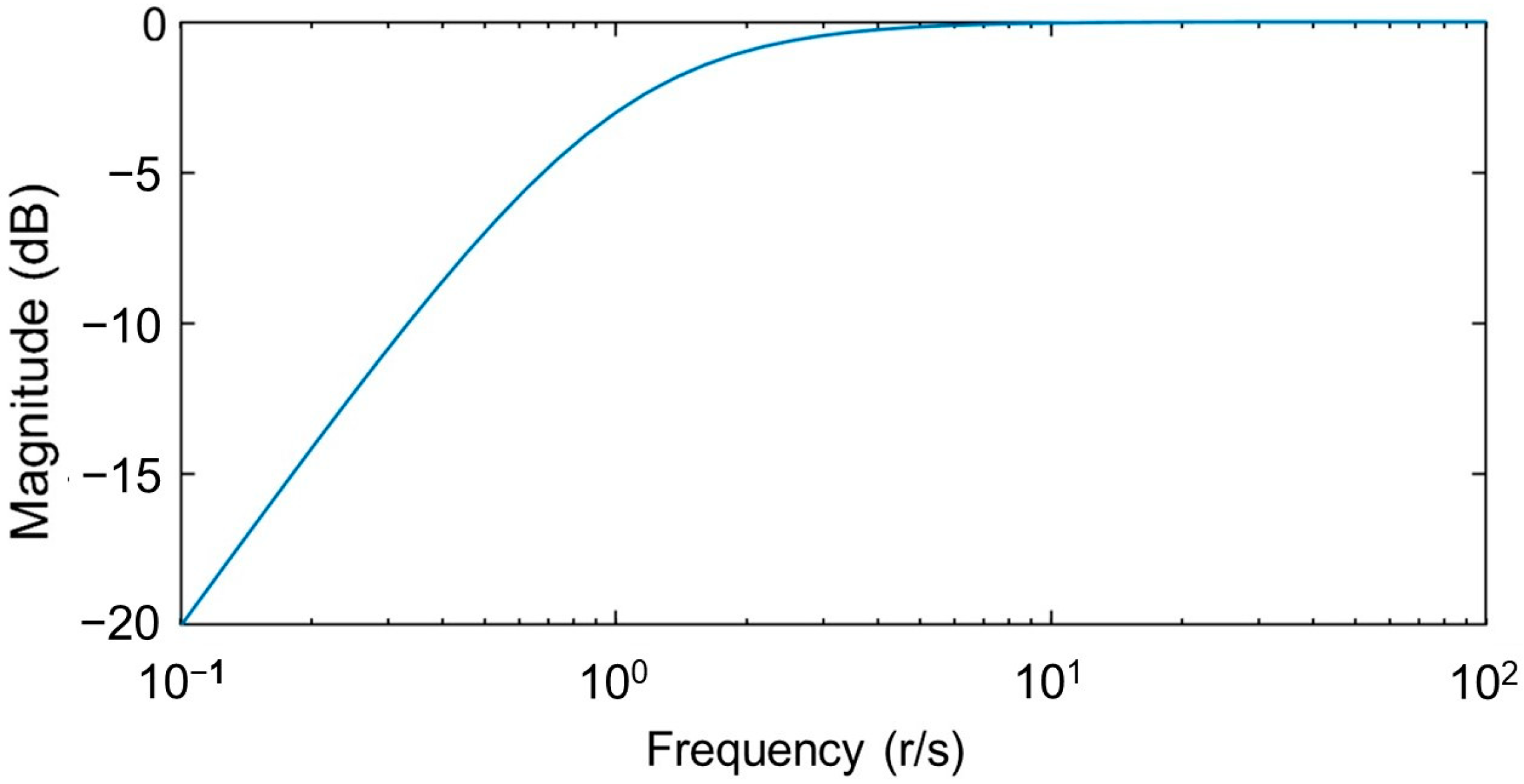
According to Equation (1), the voltage signal u(t) results from high-pass filtering of the magnetic flux Φ(t). A Bode plot of Equation (1) would simply consist of a ramp starting from very low negative dB values for frequencies close to 0 r/s and increasing constantly at a rate of 6 dB/oct. The ramp crosses the frequency axis (i.e., the gain is 0 dB) at 1 r/s and keeps growing at higher frequencies. Consequently, u(t) does not offer an accurate representation of frequency components in Φ(t). Low-frequency dynamics of Φ(t) appear minimized (filtered-out) in u(t), whereas at higher frequencies (where electromagnetic noise is often noticeable), the magnitude of components is maximized. This is not ideal, because majority of the frequency components of Φ(t) should be accurately represented in u(t). In that case, focus would be given to the lower frequency range of u(t) for detecting spectral patterns induced by load accumulation on the slab. In turn, this could ensure that any high-frequency transient electromagnetic noise would not influence the detection results.
A potential solution to this problem is provided by the circuit shown in Figure 1c, which involves a capacitor connected to a resistor in series and the pick-up coil acting as voltage source. Let the capacitor voltage be denoted by uc(t), whereas uR(t) is the voltage across the resistance R. Then,
u c t + u R t = d Φ ( t ) d t
If C denotes the capacitance, the current i(t) flowing through the circuit is equal to
i t = C · d u c ( t ) d t
Combining Equations (2) and (3) and noting that uR(t) = i(t)∙R, yields the following:
u c t + R · C · d u c ( t ) d t = d Φ ( t ) d t
Consider the (realistic) condition of zero initial values. This means that at the instant when the circuit starts to operate, the capacitor holds no charge, and no magnetic flux has yet been produced. Then Equation (4) is rewritten in the Laplace domain as follows:
U c s + R · C · s · U c s = s · Φ s
with s being the Laplace operator. Consequently, the transfer function between the voltage across the capacitor and the magnetic flux is as follows:
U c s Φ s = s R · C · s + 1 = s s ω c + 1
with cutoff frequency ωc = 1/(RC). Selecting R, C so that RC = 1 and ωc = 1 r/s (or 0.16 Hz), the Bode plot of the transfer function in Equation (6) will act as a high-pass filter, with a magnitude of −3 dB at ωc = 1 r/s, and 0 dB (or unit magnitude) over 3 r/s (0.48 Hz), as in Figure 2.
Then, any frequency components in Φ(t) may also be present in uc(t) and have the same magnitude for frequencies over 0.48 Hz. In other words, if frequencies over 0.48 Hz are considered, patterns in Φ(t) (frequency shifts or other, see Section 2.3) induced by load accumulation on the slab, may be picked up by monitoring uc(t) in the frequency domain. In the current case, a capacitor of C = 1 μF (tolerance ±10%) and a resistor of R = 1 MOhm (tolerance ±1%) have been used, for setting ωc as close to 1 as possible. Note that by having RC > 1, then ωc < 1 in (6) and the magnitude of the resulting transfer function in Bode plots will be flat for frequencies even lower than 3 r/s (0.48 Hz), but with negative dB values (i.e., magnitude values lower than 1), which is not ideal.
Note finally that, even though other solutions for obtaining magnitudes of 0 dB above 0.48 Hz may be possible, the RC-circuit currently proposed is a passive component, meaning that no external energy is required for its operation. Hence, it perfectly fits the passive contactless sensing scheme presented in this study, which avoids using modules requiring additional power sources (for instance, interrogation coils) as much as possible. For instance, a circuit to integrate u(t) in (1) would achieve a unit gain throughout the frequency range, but it would require external power for the operational amplifier involved.

2.3. Power-Based Algorithmic Design for Detecting Load Accumulation

In [33], load accumulation on the slab is shown to result in shifting of frequency peaks in signal u(t) [see (1)] at two main frequency regions (referred to as principal activity regions), namely, one around 2700 Hz and another at 5400 Hz. In [24] and especially [33], experiments with various loads at different positions on the slab, demonstrated that loads as small as 0.46 g placed 4 cm away from the clamp (a position denoted as W4, see Figure 1b) could cause statistically significant frequency shifts in both principal activity regions (and thus be detectable). Note that in [33], the pick-up coil was directly connected to the oscilloscope as in Equation (1). Thus, high-frequency components in u(t) appeared with amplified magnitudes with respect to their counterparts in Φ(t). Consequently, in [33], frequency peaks around 5400 Hz featured seemingly larger magnitudes than peaks around 2700 Hz. On the other hand, frequency peaks were hardly distinguishable below 2700 Hz. The current study aims at obtaining detection results statistically comparable to those in [33], for equally small loads (0.46 g) at position W4, but at frequencies considerably lower than 2700 Hz. This should help to avoid the potential influence of transient electromagnetic high-frequency noise on the detection results.
Note also that detection of load-induced patterns in spectral activity at lower frequencies is possible because of the modes/eigenfrequencies of the slab at these frequencies. These are easily computed using the lumped-model methodology in [35,36] (or by Finite Element Analysis, if relevant software is available). Briefly, the cantilever slab is considered to be formed by n short rigid discrete elements connected in tandem via torsion springs. Each rigid element may exhibit planar displacement/rotation according to the spring constraints at its ends. Writing Newton’s law for each rigid element and grouping all equations together allows for the derivation of the lumped model of the slab. This is essentially a matrix equation of Newton’s law valid for the entire group of rigid interconnected elements (hence the slab). Mass and stiffness (square) matrices are used in place of mass and spring values, as normally found in scalar equations of Newton’s law. Eigenfrequencies are computed using the mass and stiffness matrices. For sufficiently large number n of elements, the computed eigenfrequency values converge to those theoretically obtained in handbooks of mechanics [36]. Currently, via the slab dimensions and details in Section 2.1, the eigenfrequency values of the slab at lower frequencies start converging for n ≥ 15. Table 1 presents the eigenfrequency values up to 2700 Hz, using n = 19 discrete elements. Potential spectral activity is indicated by the existence of several modes below 2700 Hz, which could be monitored for detecting load-induced patterns. This is currently possible, because voltage uc(t) in (4)–(6) (see Section 2.2), gives an accurate description of spectral characteristics of the magnetic flux Φ(t) for frequencies higher than 0.48 Hz. This was not the case with its counterpart u(t) found in Equation (1) and used in [33].

2.3.1. Preliminary Analysis of Experimental Data Based on Stochastic AR Modeling

In order to assess the spectral characteristics of uc(t) at frequencies lower than 2700 Hz and setup a meaningful algorithm detecting load-induced spectral patterns, a number of preliminary test runs have been carried out. These involve setting the slab into vibration via pulses at frequencies sweeping from 30 to 180 Hz, at two loading configurations: a standard configuration (i.e., without load on the slab), designated as Stdn_i and another one with 0.46 g at W4, denoted as Wght_i. The index i denotes the corresponding test run. As stated in Section 2.2, the optimal excitation profile and load position/magnitude resulted from the relevant analysis carried out in [33]. Table 2 presents the characteristics of twenty test runs conducted at each configuration, whereas Figure 3 shows the magnitudes of FFT coefficients of signals uc(t) recorded by the oscilloscope:
After careful examination of Figure 3, the first remark is that additional load-induced frequency shifts are now noticeable around 1350 Hz, along with those around 2700 and 5400 Hz, as identified in [33]. Another remark is that now spectral activity around 1780 and 2200 Hz may be noted in signals from Stdn_i cases (i.e., slab without load). This is consistent with the ninth and tenth eigenfrequencies shown in Table 1. Finally, a third remark is that no prevailing peaks are visible throughout the frequency range up to 1000 Hz even though six modes seem to be in that range (see Table 1). Obviously, the last remark does not concern peaks at 50 Hz related to the AC electrical supply and two others at 190 Hz from two sets of data at the Stdn_i configuration.
Hence, replacing the data acquisition circuit of [33] with the RC-circuit presented in Section 2.2 is beneficial at least for revealing frequency peaks that in [33] had not been observed at frequencies around 1350 Hz. On the other hand, issues still arise when monitoring frequencies up to 1000 Hz. There are no frequency components with clearly larger magnitude than the rest. Thus, an algorithm for detecting loads based on frequency shifting cannot be designed. Although disappointing, this behavior seems consistent with observations made when dealing with passive contactless magnetoelastic sensor setups in the past [15,24,25,26,27]. Since such setups are based on ambient mechanical excitation (instead of input from an interrogation coil) to vibrate, their main drawback is that the magnetic flux produced is weak and only significant at high frequencies. Nonetheless, any amount of flux (however small) produced by the vibrating magnetoelastic ribbon at low frequencies, directly affects the power of the recorded signal at these frequencies. If this flux changes due to the presence of loads on the slab, then detection of load accumulation can be based on changes in the signal power inside the considered frequency region. However, it is still unclear in what manner loads on the slab impact the magnetic flux emitted by the vibrating ribbon. An answer to this question would help to identify load-induced patterns on the distribution of signal power at a given frequency region.
In order to deal with these issues, uc(t) data from the preliminary tests (as presented in Table 2) have to be analyzed inside the frequency region of interest (up to 1000 Hz). Modeling signals uc(t) resulting from test runs in Table 2, as stochastic discrete times-series data sequences by means of stochastic AutoRegressive (AR) representations, are a powerful option for answering these questions, and have been used successfully in the past [25]. Briefly, a stochastic AR representation formulates the dependence of values of a given signal y at the (discrete) time instant kT (with T being the sampling period and k designating the sample number) as a combination of past signal values up to n previous lags augmented by a random unknown value e[kT]:
y[kT] = α1y[kTT] + α2y[kT − 2∙T] + … + αny[kTnT] + e[kT]
The term e[kT] accounts for the uncertainty of the modeling process (due to noise, for instance) and forms a white noise data sequence when all samples are considered. Estimating n along with parameters α1, …, αn (via Least-Squares criteria) is a task referred to as model identification. Once an AR representation is successfully identified for a given signal, the AR poles may be used for examining the signal’s spectral characteristics at specific frequency regions. For more details on the identification task, the interested reader may refer to [25], where signals obtained in the context of a similar contactless sensing application were studied at specific frequency regions.
Analysis of uc(t) data from the preliminary tests presented in Table 2, is carried out in two steps as follows:
  • Each voltage signal uc(t) is filtered by means of a Butterworth low-pass filter (of 7-th order, with a pass frequency at 1000 Hz and cutoff of 1200 Hz at −6 dB), and subsampled at 4000 Hz;
  • Discrete-time stochastic AutoRegressive (AR) time-series representations are identified on the (filtered and subsampled) signal from step 1, and the discrete-time AR poles corresponding to specific regions of dominant frequencies are computed and plotted on the complex z-plane.
Note that at 4000 Hz, the filtered signal components are almost at −78 dB and at 5400 Hz (the first region of the unfiltered signal with significant peaks past 4000 Hz—see Figure 3) and are even smaller at −96 dB. Hence, peaks after 4000 Hz in the recorded signal (before being filtered and subsampled) have very limited influence in the filtered and subsampled signal due to aliasing. Note also that, due to the use of the RC-circuit (Section 2.2), eventual peaks after 5400 Hz in Φ(t) are not amplified in uc(t) and maintain the trend to feature decreased magnitudes at higher frequencies.
The region of interest involves frequencies up to 1000 Hz, or 0.5∙π/T r/s (with sampling time T = 1/4000 s). Figure 4 presents AR pole locations of up to 1000 Hz, associated with recorded uc(t) data from tests with unloaded (Stdn_i) and loaded (Wght_i) slab configurations, indicated with blue and red crosses, respectively. Between 200 and 600 Hz (0.1∙π/T–0.3∙π/T r/s), AR poles associated with data sets from unloaded (in blue) and loaded (in red) slabs essentially mix with respect to their z-plane locations, whereas they mostly feature similar damping factors up to 0.3. There are notable exceptions to this rule around 500 Hz (0.25 π/T r/s). On the other hand, between 600 and 1000 Hz (0.3∙π/T–0.5∙π/T r/s), AR poles associated with data from loaded slabs (in red) are noticeably more scattered on the z-plane than their (blue) counterparts (associated with data from unloaded slabs). They also exhibit highly variable damping values, ranging from 0.1 to 0.4. Then, between 600 and 1000 Hz [and perhaps between 200 and 600 Hz], power values for signals from loaded slabs should have greater dispersions due to the observed damping variations than power for signals resulting from unloaded slabs. Intuitively, this also seems reasonable, because placing a load on the slab undermines its homogeneity and symmetry. In turn, the loaded slab should handle the energy offered by the DC-vibrator in a less consistent manner, with respect to the unloaded slab.

2.3.2. Signal Power Estimation and Algorithmic Design

The power of the recorded signal inside a specific frequency range may be estimated by means of its periodogram [37]. This uses the (suitably normalized) squared magnitudes of FFT coefficients of a signal to compute its power spectral density (PSD), which essentially describes the distribution of the signal’s power at different frequencies. Integrating the PSD over frequencies allows for computing the signal power inside the considered range. In MATLAB®, this procedure is executed via the command bandpower.m, making the estimation of the signal power quite easy. Hence, carrying out a number of k test runs without load on the slab and computing signal power values inside a considered range yields a set of k power values. These correspond to a slab operating in ideal conditions, i.e., without pests or other harmful agents on its surface (and, hence, the nearby environment). Then, this set may be statistically compared with similar sets involving power values from test runs with slabs at unknown load configuration (loaded or not), in order to statistically conclude on the existence of pests or other agents on their surface. The conclusions take into account the uncertainty of the decision-making process, due to factors such as noise.
Technically, for each frequency range considered (200–600 Hz or 600–1000 Hz), the statistical comparison of two sets, namely, one resulting from Stdn (referred to as Stdn) and another from an unknown load configuration (referred to as Unkwn), can be formulated as a statistical hypothesis testing problem. If Var(X) designates the variance of set X, the hypothesis testing problem is as follows:
H0: For sets Stdn and Unkwn, it holds that Var(Stdn) = Var(Unkwn)
     H1: For sets Stdn and Unkwn, it holds that Var(Unkwn) > Var(Stdn).
In order to solve the hypothesis testing problem and choose between the null (H0) and alternative (H1) hypotheses in Equation (8), a suitable statistical test must be selected. When data in the two sets follow normal distribution, parametric statistical tests can be used. One standard test is the F-test (see Section 8.5 in [38]), specifically its one-sided variant, since the alternative hypothesis involves checking that Var(Unkwn) > Var(Stdn). If data in the two sets do not follow normal distributions, then (less powerful) non-parametric tests such as the Brown–Forsythe test (Section 11.5 in [38]) may be used. As reported in Section 3 (Results), one means for assessing the normality of small-sized data sets is via the Shapiro–Wilk test (chapter. 6 in [39]), because it is particularly well-suited to sets with less than 50 values, as is the case in this study). In all cases, the decision to choose between null and alternative hypotheses in Equation (8) is made at a given risk (or significance) level α, usually selected to be equal to 0.05. It corresponds to the probability of rejecting H0, even though it is true. In simple terms, if H0 is rejected at α = 0.05, then there is only 5% probability (risk) to accept that “variance of data in Unkwn set is larger than that of data in Stdn set”, whereas this is not true. An outline of the algorithm for statistically detecting load accumulation on the slab surface is as follows:
  • Data from k test runs conducted are filtered (via a Butterworth 7-th order low-pass filter with a pass value at 1000 Hz and stop value at 1200 Hz with −6 dB);
  • Filtered data are subsampled at 4000 Hz;
  • The power of each signal (out of k) is computed using the periodogram (or command bandpower.m in MATLAB®);
  • A set of data involving k values of signal power at the considered frequency range (200–600 Hz or 600–1000 Hz) is formed;
  • The data set in step 4 is checked for normality via the Shapiro–Wilk test;
  • Following the results of step 5, a suitable statistical test is used for comparing the current Unkwn data set with a Stdn data set, at the considered frequency range. Conclusions are drawn, accordingly, on the load detected on the slab (or not) at the α = 0.05 risk level.
Note that, other than a precise fitting/alignment of the setup during installation, no calibration between runs is necessary. The setup should operate without external intervention until pests detected on the slab. At that point, the setup should be cleaned and realigned.

3. Results

Tests conducted with the slab at unloaded or loaded configurations, referred to as Stdn_i or Wght_i in Table 2 (with i being the run number), and the relevant settings are reported in Table 3. In order to ensure that variable conditions with respect to noise are simulated, test runs took place on three different days, referred to as Day 1, Day 2 and Day 3 in Table 3. Day 1 includes all preliminary tests, since these have only been studied (via stochastic AR modeling methods) in terms of frequency characteristics, but not evaluated via the algorithm of Section 2.3.2.
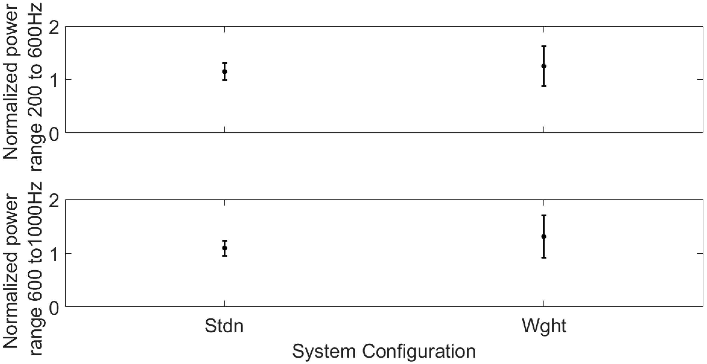
According to the six-step algorithm in Section 2.3.2, data sets from all days are initially low-pass filtered at 1000 Hz and subsampled at 4000 Hz. Then, via bandpower.m in MATLAB®, data sets involving 20 power values per configuration are formed for each of the two frequency ranges (200–600 Hz and 600–1000 Hz). Note that signal power values from runs at each configuration (Stdn_i or Wght_i, i = 1…20) are normalized with respect to the minimum power value of that set. Since relatively low-frequency ranges (200–600 or 600–1000 Hz) are considered, the noise layer should not vary much during the time these 20 tests of 5 s each are carried out. The minimum value should then include the effect of the standard noise layer and a minimum (with respect to those in the remaining 19 values) contribution from Φ(t) according to slab’s current vibration dynamics. Then normalizing to the minimum value means that the noise layer is taken as a common factor for the given load configuration, with the normalized variance of the set being mostly due to the slab’s dynamics (as affected by the load configuration). Consequently, the dispersion of normalized power values illustrates how the setup handles the standard energy provided by the DC-vibrator, mostly due to its current configuration (Stdn_i or Wght_i).
Figure 5 (top and bottom) shows representative plots of power dispersion from data recorded at Stdn_i and Wght_i configurations (i = 1…20), in the 200–600 Hz and 600–1000 Hz ranges. The limits correspond to the mean value of the data set plus/minus two standard deviations. Obviously, when the slab is loaded, the dispersion of power values increases at both ranges (200–600 Hz or 600–1000 Hz), even though at this point, it is not clear whether this result is statistically significant. Then, all sets with normalized power values from test runs in Table 3 (obtained at step 4 of the algorithm in Section 2.3.2) are assessed for normality (step 5) by means of the Shapiro–Wilk test inside both frequency ranges of interest (200–600 Hz or 600–1000 Hz). The test may be implemented in MATLAB® by adding the function swft.m as found in [40] or may even be carried out via online applications [41], with some of them directly accepting spreadsheet data [42]. Briefly, the test concludes whether the data under consideration follow normal distributions or not, by solving a hypothesis testing problem at risk level α. The null hypothesis H0 is that the data are normally distributed, whereas the alternative hypothesis H1 is that they are not. For α = 0.05, the test provides probability values (p-values), which lead to accepting H0 if they are greater than 0.05. In the current study, p-values range from 0.144 to 0.65 for the results of all test runs in Table 3 and for both frequency ranges, meaning that the null hypothesis is systematically accepted.
Given that normalized power values resulting from step 4 in Section 2.3.2 follow normal distribution, a standard parametric test to solve the hypothesis problem (8) is the one-sided F-test [38]. Briefly, the F-test compares the sample variance (namely ss2) of power values obtained at Stdn with the variance (namely su2) obtained at Unkwn configurations. The test examines the ratio ss2/su2, which should follow the F-distribution under the null hypothesis H0, at risk level α. Both numerator and denominator degrees of freedom are equal to k − 1, with k being the sample size of sets at the Stdn and Unkwn configurations, which is common in this study. The ratio is, then, compared with tabulated critical F-distribution values, related to the degrees of freedom and the selected α, in order to decide whether H0 should be accepted over H1, at the selected risk level α. In MATLAB®, the F-test is instantaneously executed via command vartest2.m, which provides p-values and the hypothesis accepted. For a risk level α = 0.05, p-values larger than 0.05 will lead to accepting H0, meaning that power values at the considered frequency range resulting from tests at Stdn and Unkwn configurations have statistically equal variances (dispersions). Then, Stdn and Unkwn configurations are similar in that they do not involve load on the slab. The p-values for all tests are presented in Table 4, along with the accepted hypothesis.
As seen in Table 4, the testing scenario simulates a realistic condition of an ideal (unloaded) slab at the beginning of Day 1, before a load of 0.46 g accumulates by the end of Day 1. Then the slab is cleaned (emptied) early on Day 2, before load again accumulates by the end of Day 2 and for the entire Day 3. In all comparisons, the correct statistical hypothesis is accepted, meaning that the power of the recorded (and duly processed as per Section 2.3.2) uc(t) signal is useful for detecting light load deposits on the slab even in (low) frequency ranges where no peaks are evident.
A remark related to the normalization approach should be formulated at this point. As stated above, variances in a set (resulting from tests at a given configuration, namely, Stdn or Wght) are normalized to the minimum of 20 values therein. Given that this approach is sensitive to outliers, an additional analysis of data sets Stdn_1, Stdn_2 and Wght_1, Wght_2 and Wght_3 has been carried out, focusing on identifying outliers. The latter are commonly considered to correspond to values in a set that are larger than the median plus three standard deviations or smaller than the median minus three standard deviations. Data sets were checked using the command isoutlier.m in Matlab®, with the analysis concluding that only outliers larger than the median plus three standard deviations were present as follows: one outlier in Stdn_1 set at 200–600 Hz, another in Stdn_1 at 600–1000 Hz and three outliers in Stdn_2 set at 200–600 Hz. In other words, no outliers were found in Wght sets at any frequency range. For these three Stdn sets, normalizing to the minimum variance value should then lead to a “worst case” scenario of a seemingly larger variance at the standard unloaded configuration. When using the hypothesis tests, this would make detection of load-induced variance in Wght sets more difficult to achieve rather than easier. In other words, the detection results may be more conservative, in the sense that a case of loaded slab may be missed. On the other hand, if outliers are present at both sets under comparison, detection is still possible as shown by the comparison between Stdn_1 (one outlier) and Stdn_2 (three outliers) at 200–600 Hz. The computed p-value of 1.421 × 10⁻¹ is comfortably larger than the risk level 0.05, and broadly similar to 1.405 × 10⁻¹, namely the p-value computed when comparing Stdn_1 (one outlier) with Stdn_2 (no outliers) at 600–1000 Hz. Hence, the correct hypothesis H0 is selected even when outliers are in both sets under comparison. Noise or other factors (related to slab alignment-see Section 4) have more impact on detection results than outliers. In the authors’ view, corrective measures to avoid outliers would involve performing more tests, for instance k = 25, at Stdn configuration and exclude a number of the resulting variance values, including those resulting from outliers, so that comparably sized sets may be formed.
Note that the results presented in Table 4 are comparable to those found in [33] and obtained by detecting of load-induced frequency shifts in data at 2.7 and 5.4 KHz. In the current case, no such shifting activity is noted between 0 and 1.3 KHz. The current results are important in that they are obtained at lower frequencies (than those in [33]), and specifically in regions (200–600 and 600–1000 Hz) where no frequency shifts are noted due to the prevalent layer of noise. Hence, high-frequency (>1000 Hz) transient electromagnetic noise cannot affect load detection. Using detection results in Table 4, confusion matrices in each frequency range (200–600 and 600–1000 Hz) may be calculated. Let TP, TN, FP and FN designate the true positive, true negative, false positive and false negative values, respectively. Note that a positive detection result is related to H0 being rejected in favor of H1 (with the opposite indicating a negative detection). The confusion matrices for detection results at α = 0.05 from tests on Day 1, 2 and 3 in the 200–600 Hz or 600–1000 Hz ranges are in Table 5.
Note that detection results at α = 0.05 are identical in the 200–600 and 600–1000 Hz ranges, meaning that the respective confusion matrices are identical too. Then TP = 3, TN = 1, FN = 0 and FP = 0 and sensitivity (=TP/(TP + FN)), specificity (TN/(TN + FP)) and accuracy ((TN + TP)/(number of all tests)) metrics are all equal to 1 in the 200–600 and 600–1000 Hz ranges. Obviously, the detection performance presented in these matrices is only indicative. Definitively, more reliable results are only obtainable if many more tests are carried out and data are processed via the power-based method at α = 0.05. Nonetheless, indications about the influence of the selected value for α can, indeed, be obtained by the calculation of the respective confusion matrices. If α = 0.01, then the results in Table 4 are slightly modified as presented in Table 6.
A simple examination of Table 4 and Table 6 (lines 6, 8) indicate that only comparisons of Stdn_1 with Wght_2 and Stdn_1 with Wght_3 in the 200–600 Hz range yield different results. The null hypothesis is accepted in both cases, meaning that two cases of loaded slabs are missed. Then, the calculated confusion matrix is as in Table 7.
Now, TP = 1, TN = 1, FN = 2, FP = 0, meaning that now sensitivity = 0.33, specificity = 1 and accuracy = 0.5. In turn, these results mean that lower risk levels α lead to decreased sensitivity and accuracy in the 200–600 Hz range. However, these performance results can reliably identify such tendencies only if many more tests are carried out and data are processed via the power-based method at various values of α. In future work, further extensive testing along with structural refinements (fittings, means of excitation, etc.) are planned so that the setup may be tested during extended periods of time, and critical measures such as its sensitivity, specificity and overall detection accuracy may be computed.

4. Discussion

An initial remark is that the set Stdn_i_1 has been used as benchmark of the ideal unloaded slab for comparisons on Day 2 and Day 3, because it corresponds to data from a thoroughly clean and precisely installed/aligned slab. It is very difficult to thoroughly clean and remove loads (especially pests and similar substances) from the slab without dismantling it. Eventual leftovers (glue, pests and so on) and, crucially, shocks to the slab (resulting in misalignments) when trying to remove leftovers will inevitably result in decreased detection performance. This is illustrated by the comparison of data from Stdn_i_1 with those from Stdn_i_2 configurations on Day 2. The null hypothesis is comfortably accepted but the computed p-value is just larger than 1.4 × 10⁻¹ both at the 200–600 and 600–1000 Hz ranges. Hence, the slab was cleaned and realigned to its initial specification, before continuing with further testing on Day 2 and 3. Obviously, this remark is only relevant to the present prototype, since this is simply built for proof-of-concept testing. Further improvements for increased operational robustness, involving better clamping solutions and/or better support for fixing the pick-up coil over the magnetoelastic ribbon, are possible and will be developed in an improved version of the setup in the future.
It is also important to view the current work as the latest part of an ongoing research effort starting with [24] and continuing with [33]. In [24], effort was invested in finding the minimal value of load and its potential position on the slab resulting in noticeable frequency shifts in the recorded data signals. A load of 0.5 g in a position as close to the ribbon as possible was the lowest that could be detected, under a frequency sweep excitation input from 120 to 180 Hz at frequency ranges around 1.3, 45 and 80 KHz. In [33], the minimal load of just under 0.5 g (actually 0.46 g) was again considered, but other positions on the slab along with seven different excitation inputs (pulses of constant frequency at 30, 60, 90, 120, 150, 180 Hz and sweeps from 30 to 180 Hz) were statistically assessed in terms of load-detection performance. This effort helped to identify position W4 as the best position for detecting 0.46 g under a frequency sweep excitation input from 30 to 180 Hz. Nonetheless, frequency shifts in data from tests with loaded slabs were statistically detectable only at frequencies around 2700 or 5400 Hz. Clearly, the Signal-to-Noise ratio (SNR) was low in both [24] and [33], especially at frequencies lower than 1300 Hz, as testified by the total absence of frequency peaks in the region of 0–1300 Hz. No load-induced frequency shifts could be detected even at W4, since signals induced by magnetic flux emitted by the ribbon were buried into prevailing ambient (mostly electromagnetic) noise—but this is a known problem with passive magnetoelastic sensor setups. Given the problematic SNR, the current effort focused on finding out whether 0.46 g could be detected at (the designated as most sensitive) position W4, but by tolerating the inevitably significant noise layer and investigating novel load-induced patterns (other than load-induced frequency shifts). The currently proposed design of the passive RC-circuit along with the power-based method proposed in Section 2.3.2 achieve the statistical detection of load-induced patterns in the recorded signal.
Currently, robustness with respect to noise is ensured by the statistical framework of the proposed power-based method: in the frequency range from 0 to 1300 Hz, minor activity (instead of no activity at all in [33]) may now be noticed due to the RC-circuit used for data acquisition, although without any significant load-induced peaks (since SNR is low). Using the power-based method, one may obtain clearly detectable load-induced patterns at a given risk level α (which quantifies the uncertainty of decision-making process). Note that testing on different days and observing the evolution of p-values in Table 4 provides insight into the existence and amount of noise during testing. On Day 2 and Day 3, although no changes on the setup or its parts were made, p-values for data from loaded slabs (i.e., Wght_i_2 and Wght_i_3) were larger than p-values for data from loaded slabs on Day 1. Even though the correct hypothesis is selected (i.e., loaded slabs are identified as such), it is obvious that more noise (signifying an even lower SNR) is present on Day 2 and Day 3, which makes the decision-making process harder. At the same time, the power-based method still performs correctly, as evidenced by the selection of the correct hypothesis. In future work, testing the power-based detection algorithm with respect to specific levels of SNRs would be a reasonable next step.
Results in Table 4 demonstrate that it is possible to monitor spectral activity in frequency ranges of low SNR where no peaks are obvious, via a low-cost passive circuit for signal acquisition and the power-based method. Nonetheless, all frequency ranges do not offer the same detection potential. Higher frequency ranges have better load detection potential, which is a weak point common to passive magnetoelastic setups. In the current case, it seems plausible that inside the 200–600 Hz range, the limits of what can be detected are reached, because p-values for data from loaded slabs are close to 0.04 and just smaller than the risk level of 0.05. On the other hand, inside the 600–1000 Hz range, p-values for the data from loaded slabs are of the order of 10−3, meaning that maybe smaller loads could be detected in that range. Distributed loads are not representative for this application, because in principle one smears a small region around W4 with pest-attracting substance precisely to concentrate their mass around a specific point. Hence, p-values can additionally offer insight into the load value that can be detected by using the current setup.
As stated in Section 3, results are comparable to those obtained in [33], but in quite a lower frequency range. Other signal-based devices, which are readily available for detecting pests/bugs in constrained places do not seem available, to the best of the authors’ knowledge. Detection results with a purposely designed device based on the active principle (i.e., with an additional interrogation coil) is out of the scope of this work, since adding hardware and complexity would undermine the cost-effective nature of the currently proposed setup. If such an active device were to be developed, it could by definition offer better detection performance. However, its development would suggest doubling the available equipment (a second coil, powerful enough to set the suspended ribbon into vibration, a power amplifier and sources with dedicated circuitry for driving the coil, etc.).
In contrast to the active approach, the passive approach offers simple/rugged construction (the ribbon is fixed on a slab, which can be cleaned easily, if properly fixed) and limited power demand (one source for the acquisition device, one battery for the Arduino® Uno microprocessor), whereas the power-based detection may be easily coded using conventional software. As this proof-of-concept study suggests, promising results (Table 4) via this basic setup are possible if a suitable load detection algorithm is used. At the current stage of development, the setup involves the following components with the approximate costs being indicative to the country/market of reference: A pick-up coil VISHAY IWAS-3827EC-50 (5 Eu), an Arduino® Uno (15 Eu), a polymer slab (up to 2 Eu), a vice for fixing the slab in a cantilever arrangement (10 Eu), a capacitor with C = 1 μF (tolerance of ±10%) and resistor with R = 1 MOhm (tolerance of ±1%) for composing the RC-circuit on a breadboard (5 Eu for the complete RC-circuit), a short Metglas® 2826MB ribbon (10 Eu/kg, hence less than 1 Eu), the DC-vibrator (3 Eu), cables and a simple two-channel oscilloscope (50 Eu). A laptop should always be available for any signal-based remote detection setup, whereas coding the power-base method is simple enough in most software packages. In total, this seems like quite a cost-effective basis for an experimental setup.

5. Conclusions

An experimental setup making use of the magnetoelastic characteristics of Metglas® 2826MB ribbons for obtaining the contactless detection of pest/substance accumulation in confined spaces is enhanced in terms of performance and robustness via both hardware and algorithmic development. Its design features the standard configuration of passive contactless sensing setups: A short thin polymer slab fixed as cantilever with a short ribbon attached to its surface near the clamped end, with excitation at the other end generating vibration and thus, magnetic flux from the ribbon. A pick-up coil, suspended above the ribbon, transforms the flux into voltage, which is then monitored for spectral changes induced by load accumulating on the slab surface. However, in the current application a new passive circuit is proposed so that the recorded voltage may exhibit spectral dynamics identical to those of the flux at frequencies over 0.48 Hz. Hence, it is now possible to monitor spectral changes at significantly lower frequencies than before. This property is fully exploited by a novel algorithm, which uses the power of recorded voltage for statistically detecting spectral changes in such low frequencies, even when noise is prevalent. Consequently, one of the main issues of passive contactless sensing setups, namely that detection is only possible at higher frequencies, is now addressed. The obvious benefits are in the performance of load detection performance at low frequencies and, correspondingly, the robustness to transient high-frequency noise. Extensive testing of the proposed setup on different occasions demonstrates that loads equal to 0.46 g (and possibly even less) can be robustly detected under various conditions. These results are promising, especially given the simple cost-efficient built via conventional hardware of the setup. Future work should focus on extensive testing over many occasions and various environments to compute reliable values for sensitivity, specificity and overall detection accuracy. Again, alternative detection methodologies such as machine learning could be explored for delivering load detection results and serve as benchmark to the power-based method currently introduced.

Author Contributions

Conceptualization, D.D.; methodology, D.D. and I.K.; software, I.K.; validation, I.K.; formal analysis, D.D. and I.K.; investigation, D.D.; resources, D.D.; data curation, I.K.; writing—original draft preparation, D.D.; visualization, I.K. and D.D.; supervision, D.D.; project administration, D.D. All authors have read and agreed to the published version of the manuscript.

Funding

This research received no external funding.

Data Availability Statement

Data are available on a personal need basis by contacting the corresponding author of the published article and upon agreement with the authors.

Conflicts of Interest

The authors declare no conflicts of interest.

References

  1. Michalski, S. Care and preservation of collections. In Running a Museum: A Practical Handbook; Boylan, P.J., Ed.; ICOM—International Council of Museums, Maison de l’UNESCO: Paris, France, 2004; pp. 51–90. [Google Scholar]
  2. Querner, P. Insect Pests and Integrated Pest Management in Museums, Libraries and Historic Buildings. Insects 2015, 6, 595–607. [Google Scholar] [CrossRef] [PubMed]
  3. Pinniger, D. Past, present and future: Changes in status and distribution of museum insect pests. In Proceedings of the Integrated Pest Management (IPM) in Museums, Archives and Historic Houses—International Conference in Vienna, Vienna, Austria, 5–7 June 2013; Querner, P., Pinniger, D., Hammer, A., Eds.; pp. 20–30. Available online: https://museumpests.net/wp-content/uploads/2016/03/Vienna_IPM_1SM.pdf (accessed on 5 October 2025).
  4. Le Bras, Y.; Greneche, J.M. Magneto-elastic resonance: Principles, modeling and applications. In Resonance; Awrejcewicz, J., Ed.; IntechOpen: London, UK, 2017. [Google Scholar] [CrossRef]
  5. Hristoforou, E.; Ktena, A. Magnetostriction and magnetostrictive materials for sensing applications. J. Magn. Magn. Mater. 2007, 316, 372–378. [Google Scholar] [CrossRef]
  6. Grimes, C.A.; Roy, S.C.; Cai, Q. Theory, instrumentation and applications of magnetoelastic resonance sensors: A review. Sensors 2011, 11, 2809–2844. [Google Scholar] [CrossRef] [PubMed]
  7. Ren, L.; Yu, K.; Tan, Y. Applications and advances of magnetoelastic sensors in biomedical engineering: A review. Materials 2019, 12, 1135. [Google Scholar] [CrossRef]
  8. Lopes, A.C.; Sagasti, A.; Lasheras, A.; Muto, V.; Gutiérrez, J.; Kouzoudis, D.; Barandiarán, J.M. Accurate Determination of the Q Quality Factor in Magnetoelastic Resonant Platforms for Advanced Biological Detection. Sensors 2018, 18, 887. [Google Scholar] [CrossRef]
  9. Grimes, C.A.; Jain, M.K.; Singh, R.S.; Cai, Q.; Mason, A.; Takahata, K.; Gianchandani, Y. Magnetoelastic microsensors for en-vinronmental monitoring. In Proceedings of the 14th IEEE International Conference on Micro Electro Mechanical Systems (MEMS), Interlaken, Switzerland, 21–25 January 2001; pp. 278–281. [Google Scholar] [CrossRef]
  10. Baimpos, T.; Boutikos, P.; Nikolakakis, V.; Kouzoudis, D. A polymer-Metglas sensor used to detect volatile organic compounds. Sens. Actuator A Phys. 2010, 158, 249–253. [Google Scholar] [CrossRef]
  11. Atalay, S.; Izgi, T.; Kolat, V.S.; Erdemoglu, S.; Orhan, O.I. Magnetoelastic humidity sensors with TiO2 nanotube sensing layers. Sensors 2020, 20, 425. [Google Scholar] [CrossRef]
  12. Grimes, C.A.; Kouzoudis, D. Remote query measurement of pressure, fluid-flow velocity and humidity using magnetoelastic thick-film sensors. Sens. Actuators A Phys. 2000, 84, 205–212. [Google Scholar] [CrossRef]
  13. Grimes, C.A.; Kouzoudis, D.; Dickey, E.C.; Qian, D.; Anderson, M.A.; Shahidian, R.; Lindsey, M.; Green, L. Magnetoelastic sensors in combination with nanometer-scale honey combed thin film ceramic TiO2 for remote query measurement of humidity. J. Appl. Phys. 2000, 87, 5341–5343. [Google Scholar] [CrossRef]
  14. Samourgkanidis, G.; Nikolaou, P.; Gkovosdis-Louvaris, A.; Sakellis, E.; Blana, I.M.; Topoglidis, E. Hemin-modified SnO2/Metglas electrodes for the simultaneous electrochemical and magnetoelastic sensing of H2O2. Coatings 2018, 8, 284. [Google Scholar] [CrossRef]
  15. Dimogianopoulos, D.G. Sensors and energy harvesters utilizing the magnetoelastic principle: Review of characteristic applica-tions and patents. Recent Pat. Elec. Eng. 2012, 5, 103–119. [Google Scholar] [CrossRef]
  16. Sagasti, A.; Gutiérrez, J.; Lasheras, A.; Barandiarán, J.M. Size Dependence of the Magnetoelastic Properties of Metallic Glasses for Actuation Applications. Sensors 2019, 19, 4296. [Google Scholar] [CrossRef] [PubMed]
  17. Skinner, W.S.; Zhang, S.; Guldberg, R.E.; Ong, K.G. Magnetoelastic Sensor Optimization for Improving Mass Monitoring. Sensors 2022, 22, 827. [Google Scholar] [CrossRef] [PubMed]
  18. Atalay, S.; Inan, O.O.; Kolat, V.S.; Izgi, T. Influence of Ferromagnetic Ribbon Width on Q Factor and Magnetoelastic Resonance Frequency. Acta Phys. Pol. A 2021, 139, 159–163. [Google Scholar] [CrossRef]
  19. Ren, L.; Cong, M.; Tan, Y. An Hourglass-Shaped Wireless and Passive Magnetoelastic Sensor with an Improved Frequency Sensitivity for Remote Strain Measurements. Sensors 2020, 20, 359. [Google Scholar] [CrossRef]
  20. Saiz, P.G.; Gandia, D.; Lasheras, A.; Sagasti, A.; Quintana, I.; Fdez-Gubieda, M.L.; Gutiérrez, J.; Arriortua, M.I.; Lopes, A.C. Enhanced mass sensitivity in novel magnetoelastic resonators geometries for advanced detection systems. Sens. Actuators B Chem. 2019, 296, 126612. [Google Scholar] [CrossRef]
  21. Saiz, P.G.; Porro, J.M.; Lasheras, A.; Fernández de Luis, R.; Quintana, I.; Arriortua, M.I.; Lopes, A.C. Influence of the magnetic domain structure in the mass sensitivity of magnetoelastic sensors with different geometries. J. Alloys Compd. 2021, 863, 158555. [Google Scholar] [CrossRef]
  22. Saiz, P.G.; Porro, J.M.; Lasheras, A.; Fernández de Luis, R.; Quintana, I.; Arriortua, M.I.; Lopes, A.C. Magnetoelastic ResonanceSensors: Principles, Applications, and Perspectives. ACS Sens. 2022, 7, 1248–1268. [Google Scholar] [CrossRef] [PubMed]
  23. Samourgkanidis, G.; Kouzoudis, D.; Charalambous, P.; Adnan, E. Signal Enhancement in Magnetoelastic Ribbons Through Thermal Annealing: Evaluation of Magnetic Signal Output in Different Metglas Materials. Sensors 2025, 25, 3722. [Google Scholar] [CrossRef]
  24. Dimogianopoulos, D.G.; Mouzakis, D.E. A Versatile Interrogation-Free Magnetoelastic Resonator Design for Detecting Deterioration-Inducing Agents. In Proceedings of the 1st International Conference on Structural Damage Modelling and Assessment, Ghent University, Belgium, 4–5 August 2020; Abdel Wahab, M., Ed.; Lecture Notes in Civil Engineering. Springer: Singapore, 2021; Volume 110. [Google Scholar] [CrossRef]
  25. Sultana, R.G.; Davrados, A.; Dimogianopoulos, D. Evaluating contact-less sensing and fault diagnosis characteristics in vibrating thin cantilever beams with MetGlas® 2826MB ribbon. Vibration 2024, 7, 36–52. [Google Scholar] [CrossRef]
  26. Dimogianopoulos, D.G.; Charitidis, P.J.; Mouzakis, D.E. Inducing damage diagnosis capabilities in carbon fiber reinforced polymer composites by magnetoelastic sensor integration via 3D printing. Appl. Sci. 2020, 10, 1029. [Google Scholar] [CrossRef]
  27. Dimogianopoulos, D.G.; Mouzakis, D.E. Nondestructive Contactless Monitoring of Damage in Joints between Composite Structural Components Incorporating Sensing Elements via 3D-Printing. Appl. Sci. 2021, 11, 3230. [Google Scholar] [CrossRef]
  28. Samourgkanidis, G.; Kouzoudis, D. A pattern matching identification method of cracks on cantilever beams through their bending modes measured by magnetoelastic sensors. Theor. Appl. Fract. Mech. 2019, 103, 102266. [Google Scholar] [CrossRef]
  29. Samourgkanidis, G.; Kouzoudis, D. Characterization of magnetoelastic ribbons as vibration sensors based on the measured natural frequencies of a cantilever beam. Sens. Actuator A Phys. 2020, 301, 111711. [Google Scholar] [CrossRef]
  30. Samourgkanidis, G.; Kouzoudis, D. Magnetoelastic Ribbons as Vibration Sensors for Real-Time Health Monitoring of Rotating Metal Beams. Sensors 2021, 21, 8122. [Google Scholar] [CrossRef]
  31. Tapeinos, C.I.; Kamitsou, M.D.; Dassios, K.G.; Kouzoudis, D.; Christogerou, A.; Samourgkanidis, G. Contactless and Vibration-Based Damage Detection in Rectangular Cement Beams Using Magnetoelastic Ribbon Sensors. Sensors 2023, 23, 5453. [Google Scholar] [CrossRef]
  32. Kouzoudis, D.; Samourgkanidis, G.; Tapeinos, C.I. Contactless Detection of Natural Bending Frequencies using Embedded Metallic-Glass Ribbons inside Plastic Beams made of 3-D Printing. Recent Prog. Mater. 2021, 3, 010. [Google Scholar] [CrossRef]
  33. Kalyvas, I.; Dimogianopoulos, D. Optimizing Contact-Less Magnetoelastic Sensor Design for Detecting Substances Accumulating in Constrained Environments. Designs 2024, 8, 112. [Google Scholar] [CrossRef]
  34. García-Arribas, A.; Gutiérrez, J.; Kurlyandskaya, G.V.; Barandiarán, J.M.; Svalov, A.; Fernández, E.; Lasheras, A.; de Cos, D.; Bravo-Imaz, I. Sensor Applications of Soft Magnetic Materials Based on Magneto-Impedance, Magneto-Elastic Resonance and Magneto-Electricity. Sensors 2014, 14, 7602–7624. [Google Scholar] [CrossRef]
  35. Tůma, J.; Škutová, J. Simulation of active vibration control of the cantilever beam. In Proceedings of the 13th International Carpathian Control Conference (ICCC), High Tatras, Slovakia, 28–31 May 2012; pp. 744–747. [Google Scholar] [CrossRef]
  36. Tuma, J.; Mahdal, M.; Suranek, P. Simulation study of the non-collocated control of a cantilever beam. Mech. Control. 2013, 32, 110–116. [Google Scholar] [CrossRef]
  37. Ljung, L. System Identification: Theory for the User; Prentice-Hall: Upper Saddle River, NJ, USA, 1999. [Google Scholar]
  38. Zar, J.H. Biostatistical Analysis, 5th ed.; Prentice Hall: Upper Saddle River, NJ, USA, 2010. [Google Scholar]
  39. Hoffman, J.I.E. Basic Biostatistics for Medical and Biomedical Practitioners, 2nd ed.; Elsevier Science: Amsterdam, The Netherlands, 2019; ISBN 978-0-12-817084-7. [Google Scholar] [CrossRef]
  40. Gardner-O’Kearney, W. swft—Shapiro-Wilk/Shapiro-Francia Tests. 2021. Available online: https://www.mathworks.com/matlabcentral/fileexchange/88778-swft-shapiro-wilk-shapiro-francia-tests (accessed on 19 September 2025).
  41. Shapiro-Wilk Test. Available online: https://www.statskingdom.com/shapiro-wilk-test-calculator.html (accessed on 19 July 2025).
  42. Shapiro-Wilk Test. Available online: https://www.sthda.com/english/rsthda/shapiro-wilk.php (accessed on 19 July 2025).
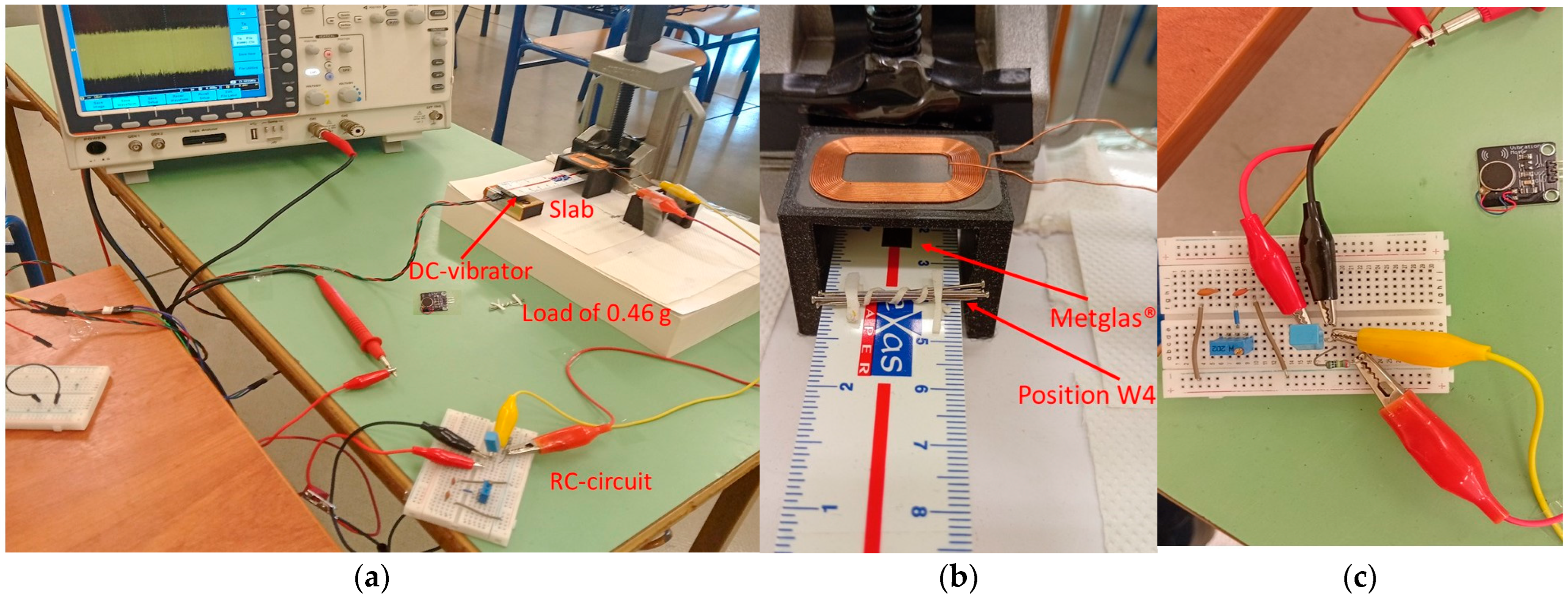
Figure 1. The detection setup: (a) the polymer slab clamped under the pick-up coil with the DC-vibrator at the opposite end, with a load of 0.46 g ready to be fixed and the RC-circuit processing data to be recorded by the oscilloscope; (b) the pick-up coil over the Metglas® ribbon and the load fixed at position W4; (c) the RC-circuit with the DC-vibrator on the right.
Vibration 08 00064 g001
Figure 2. Bode magnitude plot of transfer function (6), showing a high-pass filter behavior but with unit gain (due to magnitude values equal to 0 dB) for frequencies higher than 3 r/s (0.48 Hz).
Vibration 08 00064 g002
Figure 3. Fast Fourier Transform for uc(t) data recorded during preliminary tests with and without load (Stdn and Wght, respectively) on the slab (20 test runs per case); frequency shifts in three main regions (1350, 2700 and 5400 Hz) clearly indicate load accumulation on the slab surface.
Vibration 08 00064 g003
Figure 4. AR poles on the complex z-plane up to 1000 Hz associated with (filtered and subsampled at 4000 Hz) uc(t) data from unloaded (Stdn_i) and loaded (Wght_i) slab configurations: poles associated with Wght_i have greater dispersions mostly between 600 and 1000 Hz (0.3∙π/T–0.5∙π/T r/s) and, to a lesser extent, between 200 and 600 Hz (0.1∙π/T–0.3∙π/T r/s).
Vibration 08 00064 g004
Figure 5. Dispersion of power values for data from unloaded (Stdn_i) and loaded (Wght_i) test runs, showing that dispersion increases for loaded slabs both in 200–600 Hz and 600–1000 Hz ranges.
Vibration 08 00064 g005
Table 1. Modes and their frequency values for the considered slab up to 2700 Hz.
ModeFrequency (Hz)
18.7
254.6
3153.1
4300.4
5497.1
6743.3
71038.8
81383.1
91775.4
102213.6
112694.2
Table 2. Configuration and details of preliminary tests.
ConfigurationLoad of 0.46 g (Yes/No)Sampling RateDuration (s)
Stdn_i (i = 1…20)No200 KHz5
Wght_i (i = 1…20)Yes200 KHz5
Table 3. Configuration and details of test runs on Days 1, 2 and 3 for the associated data recorded and processed as per Section 2.3.2.
Test DayConfigurationLoad of 0.46 g (Yes/No)Sampling RateDuration (s)
Day 1Stdn_i_1 (i = 1…20)No200 KHz5
Wght_i_1 (i = 1…20)Yes200 KHz5
Day 2Stdn_i_2 (i = 1…20)No200 KHz5
Wght_i_2 (i = 1…20)Yes200 KHz5
Day 3Wght_i_3 (i = 1…20)Yes200 KHz5
Table 4. Accepted hypothesis at α = 0.05 and p-values computed by one-sided F-test for comparisons of data recorded from test runs at Day 1, 2 and 3 and processed as per Section 2.3.2.
Test DayComparison Stdn vs. UnkwnLoad of 0.46 g Stdn–UnkwnFrequency RangeAccepted Hypothesis—p-Value
Day 1Stdn_i_1 vs. Wght_i_1 (i = 1…20)No–Yes200–600 HzH1—2.97 × 10⁻⁴
Stdn_i_1 vs. Wght_i_1 (i = 1…20)No–Yes600–1000 HzH1—2.15 × 10⁻⁵
Day 2Stdn_i_1 vs. Stdn_i_2 (i = 1…20)No–No200–600 HzH0—1.421 × 10⁻¹
Stdn_i_1 vs. Stdn_i_2 (i = 1…20)No–No600–1000 HzH0—1.405 × 10⁻¹
Stdn_i_1 vs. Wght_i_2 (i = 1…20)No–Yes200–600 HzH1—3.9 × 10⁻²
Stdn_i_1 vs. Wght_i_2 (i = 1…20)No–Yes600–1000 HzH1—8.62 × 10⁻⁵
Day 3Stdn_i_1 vs. Wght_i_3 (i = 1…20)No–Yes200–600 HzH1—3.38 × 10⁻²
Stdn_i_1 vs. Wght_i_3 (i = 1…20)No–Yes600–1000 HzH1—6.4 × 10⁻³
Table 5. Confusion matrix for detection results at α = 0.05 from tests on Day 1, 2 and 3 in the 200–600 Hz or 600–1000 Hz ranges.
Predicted Positive (H1)
(3 Instances)
Predicted Negative (H0)
(1 Instance)
Actual Positive (H1)
(3 instances)
30
Actual Negative (H0)
(1 instance)
01
Table 6. Accepted hypothesis at α = 0.01 and p-values computed by one-sided F-test for comparisons of data recorded from test runs at Day 1, 2 and 3 and processed as per Section 2.3.2.
Test DayComparison Stdn vs. UnkwnLoad of 0.46 g Stdn–UnkwnFrequency RangeAccepted Hypothesis—p-Value
Day 1Stdn_i_1 vs. Wght_i_1 (i = 1…20)No–Yes200–600 HzH1—2.97 × 10⁻⁴
Stdn_i_1 vs. Wght_i_1 (i = 1…20)No–Yes600–1000 HzH1—2.15 × 10⁻⁵
Day 2Stdn_i_1 vs. Stdn_i_2 (i = 1…20)No–No200–600 HzH0—1.421 × 10⁻¹
Stdn_i_1 vs. Stdn_i_2 (i = 1…20)No–No600–1000 HzH0—1.405 × 10⁻¹
Stdn_i_1 vs. Wght_i_2 (i = 1…20)No–Yes200–600 HzH0—3.9 × 10⁻²
Stdn_i_1 vs. Wght_i_2 (i = 1…20)No–Yes600–1000 HzH1—8.62 × 10⁻⁵
Day 3Stdn_i_1 vs. Wght_i_3 (i = 1…20)No–Yes200–600 HzH0—3.38 × 10⁻²
Stdn_i_1 vs. Wght_i_3 (i = 1…20)No–Yes600–1000 HzH1—6.4 × 10⁻³
Table 7. Confusion matrix for detection results at α = 0.01 from tests on Day 1, 2 and 3 in the 200–600 Hz range.
Predicted Positive (H1)
(1 Instance)
Predicted Negative (H0)
(3 Instances)
Actual Positive (H1)
(3 instances)
12
Actual Negative (H0)
(1 instance)
01
Disclaimer/Publisher’s Note: The statements, opinions and data contained in all publications are solely those of the individual author(s) and contributor(s) and not of MDPI and/or the editor(s). MDPI and/or the editor(s) disclaim responsibility for any injury to people or property resulting from any ideas, methods, instructions or products referred to in the content.