Stochastic Vibration of Damaged Cable System Under Random Loads

Abstract

This study proposes an integrated framework that combines nonlinear stochastic vibration analysis with reliability assessment to address the safety issues of cable systems under damage conditions. First of all, a mathematical model of the damaged cable is established by introducing damage parameters, and its static configuration is determined. Using the Pearl River Huangpu Bridge as a case study, the accuracy of the analytical solution for the cable’s sag displacement is validated through the finite difference method (FDM). Furthermore, a quantitative relationship between the damage parameters and structural response under stochastic excitation is developed, and the nonlinear stochastic dynamic equations governing the in-plane and out-of-plane motions of the damaged cable are derived. Subsequently, a Gaussian Radial Basis Function Neural Network (GRBFNN) method is employed to solve for the steady-state probability density function of the system response, enabling a detailed analysis of how various damage parameters affect structural behavior. Finally, the First-Order and Second-Order Reliability Method (FORM/SORM) are used to compute the reliability index and failure probability, which are further validated using Monte Carlo simulation (MCS). Results show that the severity parameter η shows the highest sensitivity in influencing the failure probability among the damage parameters. For the system of the Pearl River Huangpu bridge, an increase in the damage extent δ from 0.1 to 0.4 can reduce the reliability-based service life of by approximately 40% under fixed values of the damage severity and location, and failure risk is highest when the damage is located at the midspan of the cable. This study provides a theoretical framework from the point of stochastic vibration for evaluating the response and associated reliability of mechanical systems; the results can be applied in practice with guidance for the engineering design and avoid potential damages of suspended cables.

1. Introduction

Suspension structures, widely used in major infrastructure projects for their excellent mechanical properties and aesthetic value, are prone to damage such as corrosion, fatigue cracks, and broken wires as they age. These damages can significantly compromise load-bearing capacity and safety. Therefore, systematically analyzing and assessing damaged suspension structures is crucial for ensuring long-term safety and developing effective maintenance strategies.

In recent years, suspension structures have expanded from traditional bridge engineering to large-scale public facilities like sports venues and exhibition halls. Damage or destruction of such structures can lead to significant economic losses and casualties. Despite advancements in damage assessment methods, including finite element analysis and machine learning-based models, challenges remain in areas such as theoretical support, modeling complexity, and predictive accuracy related to dynamic response, reliability assessment, and the coupling of damage parameters. These issues highlight the need for further advancements.

1.1. Detection Technology for Damaged Cables

Research has shown that suspended cable structures, as flexible systems, are highly sensitive to vibrations. Damage detection technology for these structures has evolved from traditional stress–strain monitoring to a focus on vibration analysis techniques emphasizing modal characteristics. For instance, addressing the challenge of non-visually detecting corrosion in main cables, Sloane and Betti et al. (2013) [1] introduced time-domain reflectometry (TDR) for non-destructive testing, thereby significantly enhancing the ability to identify latent damage in cables. With respect to emerging technologies, machine learning algorithms are being progressively integrated into bridge damage prediction models. In their study, Feng and Gao et al. (2022) [2] proposed a novel framework for predicting cable damage. This framework integrates the effects of corrosion and fire, employing least squares support vector machines (LS-SVMs) to construct a proxy model. This approach offers a novel, data-driven method for assessing damage in complex environments. Additionally, Morgado et al. (2015) [3] studied the fatigue damage evolution process of prestressed steel cables through failure analysis, while Li et al. (2012) [4] applied acoustic emission technology to fatigue monitoring of corroded cables, providing real-time monitoring methods for damage evolution during service. Systematic methods for quantifying damage effects, coupling mechanisms, and physically-based damage evolution remain lacking despite progress in structural damage modeling.

1.2. Dynamic Analysis for Undamaged Cables

In the domain of random vibration analysis of undamaged cable systems, extant research has established a relatively comprehensive theoretical framework. The approach proposed by Gao et al. (2009) [5] utilizes random finite element analysis (RFM) to derive expressions for modal characteristics and response statistics. This method involves decomposing the structural stiffness and mass matrices into the product of random factors and deterministic matrices. Larsen et al. (2015) [6] conducted wind tunnel experiments to investigate the response mechanisms of flexible cable structures under wind excitation. Concurrently, Sun et al. (2022) [7] conducted a systematic review of the large-amplitude vibration issues of cable-stayed structures under low-damping conditions, and provided a comprehensive summary of the current status of vibration control technology development.

In comparison with undamaged systems, research on the random vibration response of damaged cable structures remains in its infancy. In their seminal work, Lan et al. (2025) [8] established a nonlinear dynamic model of damaged cables under Gaussian white noise excitation. This pioneering study addressed structural damage caused by material aging and overloading, thereby laying the theoretical foundation for systematic vibration characteristic prediction. He et al. (2024) [9] proposed a single-cable damage identification method based on vehicle-induced tension ratios, thereby overcoming the limitations of traditional multi-cable cross-validation. While undamaged system responses are well understood, studies on the dynamic behavior and reliability of damaged cable systems remain limited.

1.3. Neural Networks in the Damage Detection of Cables

In recent years, neural networks, especially deep learning models, have advanced structural damage detection in suspension systems, enabling diverse techniques and applications. Xu et al. (2021) [10] developed a hybrid model combining convolutional neural networks (CNNs) and long short-term memory (LSTM) networks, which leverages the spatial feature extraction strength of CNNs and the temporal modeling capability of LSTM. Dang et al. (2021) [11] applied message passing neural networks to damage localization in cable-stayed bridges. By utilizing the node information propagation mechanism of graph neural networks, their method successfully identified the location and severity of damage with high accuracy.

In the domain of unsupervised learning, autoencoder architectures have played a critical role in structural health monitoring. Pathirage et al. (2018) [12] proposed an autoencoder-based deep learning method for damage identification, which enabled anomaly detection without baseline data by analyzing reconstruction errors. Building upon this, Wang and Cha (2021) [13] integrated autoencoders with one-class support vector machines (OC-SVMs) to enhance the robustness of damage detection under varying conditions. In addition, Sony et al. (2019) [14] provided a comprehensive review of next-generation intelligent sensing technologies for structural health monitoring, emphasizing the advantages of machine learning algorithms in processing large-scale sensor data. Lin et al. (2017) [15] developed a deep learning-based damage detection method capable of automatic feature extraction, overcoming the limitations of traditional approaches that rely heavily on manual feature engineering. Despite the advancements above, challenges remain in improving neural network generalization under complex environmental disturbances, enhancing computational efficiency, and ensuring the physical interpretability of model outputs.

1.4. Research on the Reliability of Damaged Cables

In the reliability assessment of damaged cable structures, researchers have developed probabilistic models incorporating various deterioration mechanisms. Li et al. (2021) [16] proposed a multiscale probabilistic framework for assessing the safety of corroded main cables in long-span suspension bridges, accounting for length and Daniels effects. Wang et al. (2021) [17] developed a time-dependent reliability method for corrosion-fatigue analysis, emphasizing failure probability in short hangers under traffic loads and environmental degradation.

Health monitoring technologies for suspension structures have evolved from traditional approaches to intelligent, integrated systems with broad applications [18]. Fiber optic sensing has been central to large-span bridge monitoring, as demonstrated by Chan et al. (2006) [19] on the Tsing Ma Bridge using 40 FBG sensors. Ye et al. (2014) [20] highlighted its advantages, including compactness, light weight, and resistance to electromagnetic interference. The emergence of wireless sensor networks (WSNs) has further expanded monitoring capabilities, with Abdulkarem et al. (2020) [21] emphasizing their role in urban safety. Multisensor fusion has advanced through GNSS-accelerometer systems (Xiong et al., 2017) [22] and multi-parameter deployments (Koo et al., 2013) [23]. Other techniques, such as long-gauge strain sensing (Zhang et al., 2015) [24], have proven effective for damage detection. Recent studies underscore the impact of non-stationary effects in SHM, where damage and environmental changes alter structural dynamics. Ditommaso and Ponzo (2024) [25] proposed adaptive thresholds to address this, highlighting the need for stochastic models that capture evolving behavior.

1.5. Contribution of This Study

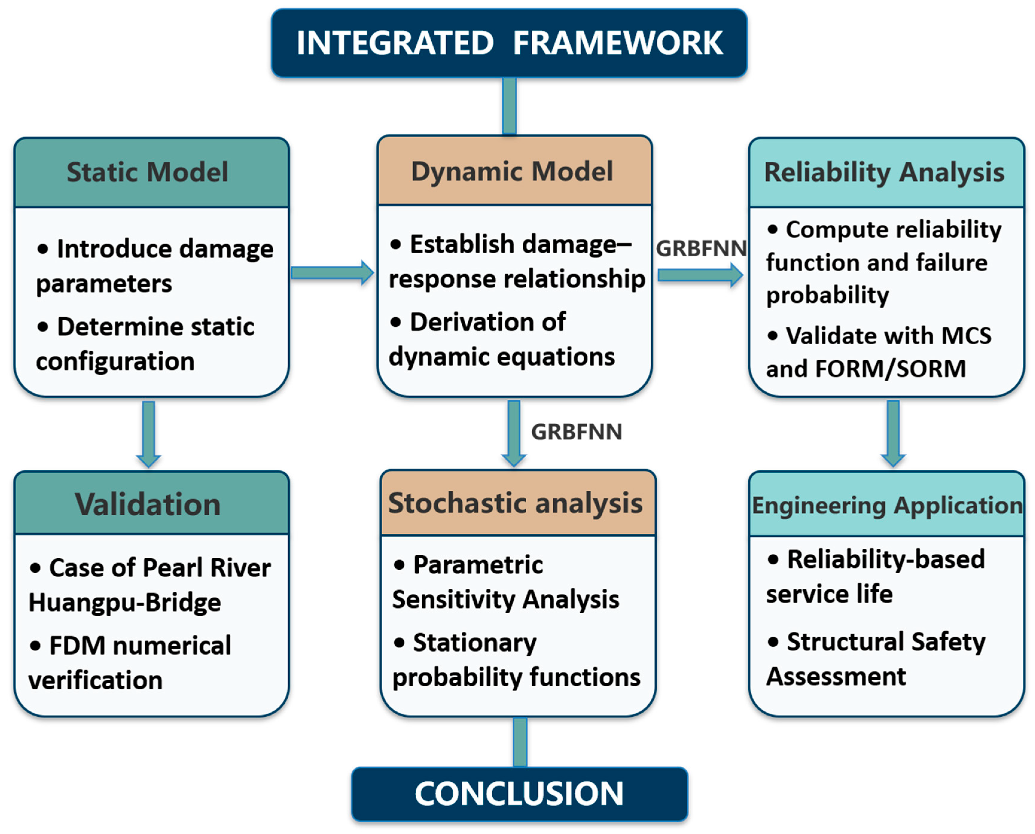
This study aims to examine the dynamic response and reliability of damaged cable structures from both theoretical and numerical perspectives. The in-plane and out-of-plane vibration equations for damaged systems are systematically derived, and a dimensionless segmented bending stiffness model is proposed. The Gaussian Radial Basis Function Neural Network (GRBFNN) is used to solve the Fokker–Planck–Kolmogorov (FPK) equation, enabling the characterization of probability density evolution under random excitation. Failure probability estimates are made using FORM/SORM, and sensitivity expressions for failure probability are derived for damage severity, extent, and location, providing a quantitative basis for damage assessment. The integrated research framework is illustrated in Figure 1.

It is important to acknowledge that this study has not yet considered the influence of material and structural nonlinearity on system behavior. Future research should continue to expand in the following areas: first, the introduction of nonlinear material properties and multi-physics coupling effects to enhance the engineering adaptability of the model; second, the development of high-precision, high-efficiency numerical algorithms to address the needs of large-scale structural analysis; and finally, the application of the modeling and assessment methods proposed in this study to apply to actual engineering projects to verify their robustness and practicality. Through the synergistic advancement of theoretical modeling, numerical analysis, and experimental validation, it is anticipated that the safety assurance level and full-lifecycle performance evaluation capabilities of suspension structures can be further enhanced.

2. Static Mathematical Modeling and Validation

2.1. Definition of Damage Parameters

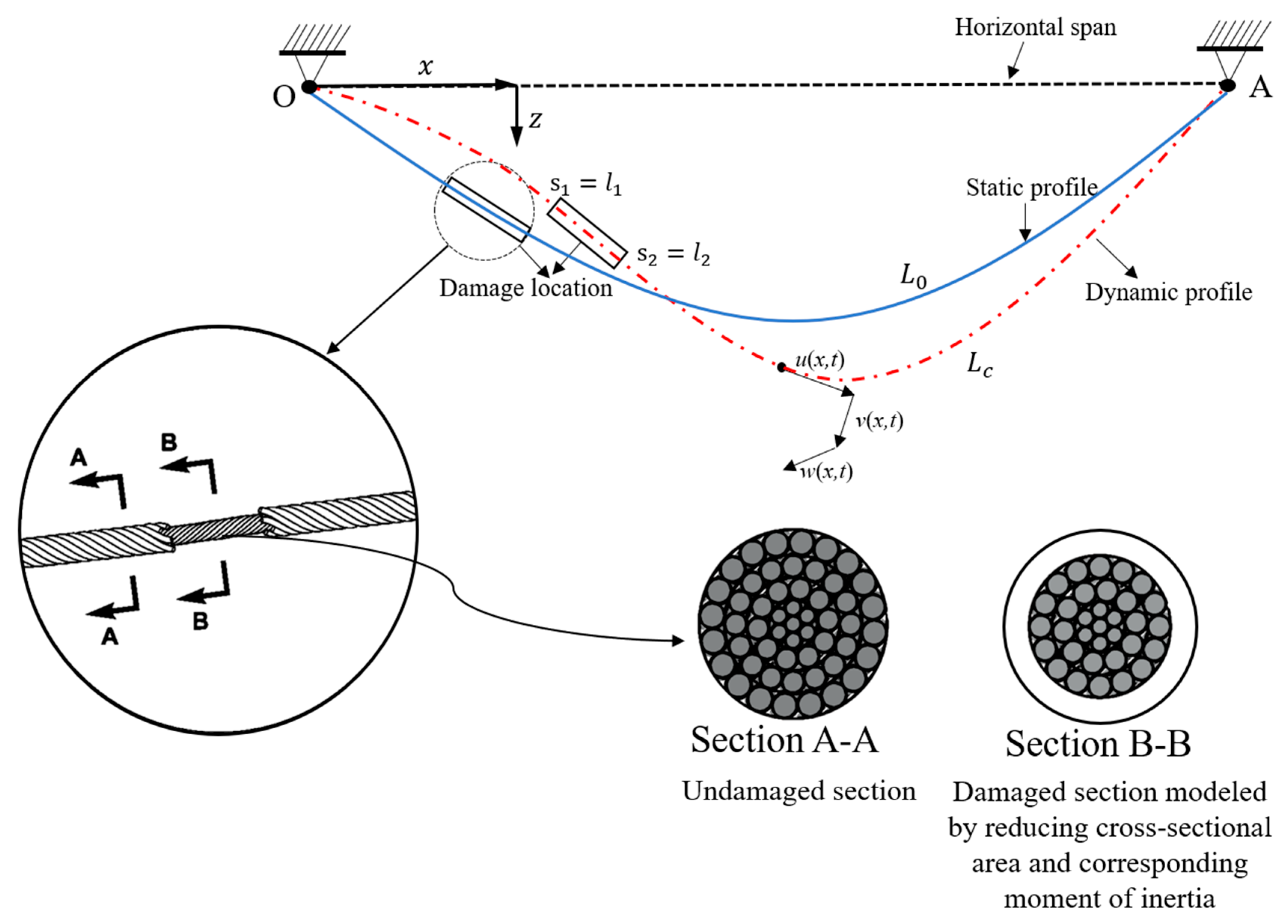
As illustrated in Figure 2, the horizontal cable system is fixed at anchor points O and A at both ends, with the natural length of the static cable in the undamaged state being $L_0$. When localized damage is introduced along the cable length direction, the local stiffness reduction caused by the damage leads to increased cable deformation, resulting in a cable length of $L_c$. Here, $z\left(s\right)$ represents the global coordinate function for any point on the suspended cable, where s denotes the arc coordinate. The damage location is positioned at a horizontal distance x from anchor point O and a vertical sagging distance z. When time-dependent external random excitation is applied to the damaged cable, the cable displacement can be decomposed into in-plane displacement $v(x,t)$ of the cable at position x and time t, out-of-plane displacement $w(x,t)$, and axial displacement $u(x,t)$. Furthermore, the flexural rigidity $EI$ is the product of elastic modulus E and moment of inertia $I$, while the axial rigidity $EA$ is the product of Young’s modulus E and cross-sectional area A.

Figure 2 also presents an enlarged view of the damage region to illustrate the physical nature of degradation. Specifically, the cable’s cross-sectional area is reduced, potentially due to degradation caused by corrosion, wire breakage, or fatigue. Cross-sections A-A and B-B, respectively, demonstrate the internal structure of the cable in undamaged and damaged states. In cross-section A-A, the cable’s interior exhibits dense arrangement and symmetric distribution, forming a robust and uniform structure. In contrast, cross-section B-B reveals missing or misaligned strands, indicating reduced load-carrying capacity.

In suspended cable structures, damage parameters primarily include damage severity, damage extent, and damage location. These parameters exert significant influence on both static displacement and dynamic response of the suspended cable. Damage severity is typically quantified through the area or volume of the damaged region; damage extent describes the distribution of damage within the suspended cable structure; damage location specifies the precise position of damage within the suspended cable structure. Variations in these parameters result in changes to the mechanical properties of the suspended cable structure, such as stiffness and mass, thereby affecting its static displacement and dynamic response. Assuming that cable damage can be represented by distributed attenuation of constant axial rigidity $EA$, the dimensionless damage severity is defined as

$$\eta \left(s\right)={\displaystyle \frac{EA-E{A}_d\left(s\right)}{EA}},0\le \eta \left(s\right)<1$$

(1)

where ${EA}_d\left(s\right)$ represents the residual axial rigidity, and $A_d\left(s\right)$ denotes the cross-sectional area at any damaged location. Assuming uniform damage severity within the damage region $s\in [l_1,l_2]$, $\eta \left(s\right)$ remains constant within the damaged region and equals zero in the undamaged region.

Therefore, the complete damage description comprises damage severity $\eta \left(s\right)$, along with the extent $\delta$ and location $\alpha$ of the damage region, which are, respectively, represented by dimensionless parameters

$$\delta ={\displaystyle \frac{l_2-l_1}{L_0}},0\le \delta \le 1, \alpha ={\displaystyle \frac{l_1+l_2}{2L_0}}, 0<\alpha <1$$

(2)

where location $\alpha$ and extent $\delta$ represent the central abscissa and length of the damage region, respectively, relative to the unstrained arc length $L_0$ of the cable in its natural configuration.

2.2. Solution of Static Equilibrium Equations

Consider a suspended cable element with horizontal span $dx$, neglecting the influence of axial stiffness and sag on the static profile, which is in equilibrium under self-weight. The self-weight of the suspended cable is uniformly distributed along its arc length. For cables with flexural rigidity, the relationship between bending moment M and curvature and the shear force $F$ generated by the rate of change of bending moment are, respectively,

$$M=EI\left(s\right){\displaystyle \frac{d^{2}z}{d{x}^2}}, F={\displaystyle \frac{d}{dx}}\left(EI\left(s\right){\displaystyle \frac{d^{2}z}{d{x}^2}}\right)$$

(3)

The vertical components $F^{\prime }$ and $T$ generated separately by the rate of change of shear force and the horizontal tension $H_s$ on the element are defined as Equation (4):

$$F^{\prime }={\displaystyle \frac{d^2}{d{x}^2}}\left(EI\left(s\right){\displaystyle \frac{d^{2}z}{d{x}^2}}\right), T=-H_s{\displaystyle \frac{d^{2}z}{d{x}^2}}$$

(4)

The suspended cable is in force equilibrium in the vertical direction, yielding the following differential equation for static deflection displacement z [26]:

$${\displaystyle \frac{d^2}{d{x}^2}}\left(EI\left(s\right){\displaystyle \frac{d^{2}z}{d{x}^2}}\right)-H_s{\displaystyle \frac{d^{2}z}{d{x}^2}}-mg=0$$

(5)

Due to the introduction of damage parameters, $EI\left(s\right)$ represents piecewise flexural rigidity, defined by damage parameters $\eta ,\delta ,\alpha$ [27]:

$$EI\left(s\right)=\left\{\begin{array}{cc}EI\left(1-\eta \right),& s\in \left[\alpha L_0-\delta L_0/2,\hspace{0.17em}\alpha L_0+\delta L_0/2\right]\\ \hspace{1em}EI,& undamaged zones\end{array}\right.$$

(6)

Let $H_s$ denote the static tension. When damage is introduced, the expression for static tension must be modified as shown in Equation (7). Here, $f_{\max }$ is a predefined constant representing the maximum allowable sag displacement in the cable design. Physically, it reflects the design constraint on vertical deflection and is typically limited to within 1/10 to 1/12 of the span length $L_0$ [28]. The term $F\left(\alpha \right)$ is an influence function associated with the damage location, given by $F\left(\alpha \right)=4\alpha (1-\alpha )$ [29].

$$H_s^{dam}={\displaystyle \frac{mg{L}_0^2}{8f_{\max }}}\cdot {\displaystyle \frac{1}{1-\eta \delta \cdot \mathcal{F}\left(\alpha \right)}},s\in \left[\alpha L_0-\delta L_0/2,\hspace{0.17em}\alpha L_0+\delta L_0/2\right]$$

(7)

After solving Equation (5), the piecewise analytical solution of differential equation for static deflection displacement z is given by Equation (8):

$$z(x)=\left\{\begin{array}{c}{A}_1\cos \mathrm{h}\left(kx\right)+B_1\sin \mathrm{h}\left(kx\right)+C_{1}x+D_1+{\displaystyle \frac{mg}{2H_s}}x\left(L_0-x\right), 0\le x<\alpha L_0-\delta L_0/2\\ A_2\cos \mathrm{h}\left(k_{d}x\right)+B_2\sin \mathrm{h}\left(k_{d}x\right)+C_{2}x+D_2+{\displaystyle \frac{mg}{2H_s^{dam}}}x\left(L_0-x\right),\alpha L_0-\delta L_0/2\le x\le \alpha L_0+\delta L_0/2\\ A_3\cos \mathrm{h}\left(kx\right)+B_3\sin \mathrm{h}\left(kx\right)+C_{3}x+D_3+{\displaystyle \frac{mg}{2H_s}}x\left(L_0-x\right), \alpha L_0+\delta L_0/2<x\le L_0\end{array}\right.$$

(8)

In the undamaged region, the parameter is defined as $k=\sqrt{H_s/EI}$, whereas in the damaged region, it becomes $k_d=\sqrt{H_s/\left[EI\left(1-\eta \right)\right]}$, where $EI$ denotes the bending stiffness in the undamaged state. When the damage parameter $\eta$ is specified, the integration constants $A_i,B_i,C_i,D_i$ can be uniquely determined using the Gaussian elimination method, based on the boundary conditions as Equation (9) and the Continuity Conditions at Damage Boundaries (at the start and end points $l_1$ and $l_2$ of the damaged region) as Equations (10)–(13).

$$z\left(0\right)=0,z\left(L_0\right)=0$$

(9)

$$z_i^{\pm }=\underset{\Delta \to 0}{\lim }z\left(l_i\pm \Delta \right),i=1,2$$

(10)

$${(z_i^{\prime })}^{\pm }=\underset{\Delta \to 0}{\lim }{z}^{\prime }\left(l_i\pm \Delta \right),i=1,2$$

(11)

$$EI\cdot {(z_i^{″})}^{\pm }=EI\left(1-\eta \right)\cdot \underset{\Delta \to 0}{\lim }{z}^{″}\left(l_i\pm \Delta \right),i=1,2$$

(12)

$${\displaystyle \frac{d}{dx}}\left[EI\cdot {(z_i^{″})}^{\pm }\right]={\displaystyle \frac{d}{dx}}\left[EI\left(1-\eta \right)\cdot \underset{\Delta \to 0}{\lim }{z}^{″}\left(l_i\pm \Delta \right)\right],i=1,2$$

(13)

Equation (10) ensures displacement continuity across the damage interface. Equation (11) enforces rotation continuity by matching the deflection slopes on both sides. Equation (12) maintains bending moment continuity, considering stiffness reduction across the interface. Equation (13) balances shear forces by ensuring the spatial derivative of the bending moment is equal on both sides, preventing unphysical accelerations in dynamic analysis.

2.3. FDM for Solving Static Displacement

The analytical method reveals the physical essence of static displacement through mathematical derivation and possesses theoretical completeness in idealized models. However, its strict requirements for geometric regularity, material linearity, and parameter constancy impose limitations in complex damage or nonlinear problems. These limitations stem from the theoretical model’s simplification of realistic conditions rather than inherent defects of the method itself. The finite difference method is employed below to verify the correctness of the analytical solution. The finite difference method transforms differential equations into computable algebraic systems through discretization strategies, overcoming the applicable boundaries of purely analytical approaches through local stiffness modification and nonlinear extension, thereby providing scientific verification for the analytical method.

The total length $L_0$ of the suspended cable is discretized into $N$ equally spaced nodes with spacing $\mathsf{\Delta }x=L_0/N$ and node coordinates $x_i=i\mathsf{\Delta }x$, $(i=0,1,\dots ,N)$. The discretized equations are written in matrix form:

$$\mathit{K}z=\mathit{F}$$

(14)

where the stiffness matrix $\mathit{K}:(N+1)\times (N+1)$ and sparse matrix with non-zero elements are determined by coefficients of the discrete equations. Displacement vector $\mathbf{z}$: $\mathbf{z}=[z_0,z_1,\dots ,z_N{]}^T$. Load vector $\mathit{F}$: $\mathit{F}=[0,mg\mathsf{\Delta }{x}_1,\hspace{0.25em}mg\mathsf{\Delta }{x}_2,\dots ,mg\mathsf{\Delta }{x}_{N-1},0]$. Incorporating all contributions, the stiffness matrix $\mathit{K}$ is a sparse banded matrix with the following specific structure:

$$\mathit{K}=\left[\begin{array}{cccccccccc}\left[a_1+{(-1)}^N{b}_1\right]& k_1& g_1& 0& \dots & \dots & \dots & \dots & \dots & 0\\ z_2& a_2& k_2& g_2& 0& \dots & \dots & \dots & \dots & 0\\ b_3& z_3& a_3& k_3& g_3& 0& \dots & \dots & \dots & 0\\ ⋮& \ddots & \ddots & \ddots & \ddots & \ddots & 0& \dots & \dots & ⋮\\ 0& \dots & b_i& z_i& a_i& k_i& g_i& 0& \dots & 0\\ ⋮& \dots & \dots & \ddots & \ddots & \ddots & \ddots & \ddots & 0& ⋮\\ 0& \dots & \dots & \dots & \dots & \dots & b_{N-1}& z_{N-1}& a_{N-1}& k_{N-1}\\ 0& \dots & \dots & \dots & \dots & \dots & \dots & b_N& z_N& \left[a_N+{(-1)}^{N+1}{g}_N\right]\end{array}\right]$$

(15)

For any point $i=1,\dots ,N$, the stiffness matrix elements in the undamaged region are given by [26]:

$$\begin{array}{c} a_i=-{\displaystyle \frac{2}{\Delta x^4}}\left(E{I}_{i+1}-5E{I}_i+E{I}_{i-1}\right)+{\displaystyle \frac{2H_s}{\Delta x^2}}\\ b_i={\displaystyle \frac{1}{2\Delta x^4}}\left(E{I}_{i+1}-2E{I}_i-E{I}_{i-1}\right)\\ g_i={\displaystyle \frac{1}{2\Delta x^4}}\left(E{I}_{i+1}+2E{I}_i-E{I}_{i-1}\right)\\ k_i=-{\displaystyle \frac{2}{\Delta x^4}}\left(3E{I}_i-E{I}_{i-1}\right)-{\displaystyle \frac{H_s}{\Delta x^2}}\\ z_i={\displaystyle \frac{2}{\Delta x^4}}\left(E{I}_{i+1}-3E{I}_i\right)-{\displaystyle \frac{H_s}{\Delta x^2}} \end{array}$$

(16)

When the damaged region is taken into consideration, the stiffness matrix elements in $\mathit{K}$ are supposed to be modified accordingly. First of all, the node indices corresponding to the damaged region are defined as

$$i_1=\alpha L_0-{\displaystyle \frac{\delta L_0}{2}}, i_2=\alpha L_0+{\displaystyle \frac{\delta L_0}{2}}$$

(17)

Therefore, bending stiffness exhibits variations across damaged versus undamaged regions, and the bending stiffness exhibits a reduction from the undamaged region to the fully damaged region. The bending stiffness is defined as $E{I}_i=EI\left(i<i_1,i>i_2\right)$ for the undamaged region and $E{I}_i=EI\left(1-\eta \right)\left(i_1<i<i_2\right)$ for the fully damaged region. Similarly, when it comes to the boundary of the damaged region, bending stiffness is not exactly the same. On the left side of the damaged region $\left(i=i_1\right)$, the bending stiffness is quantified as Equation (18); in contrast, it takes the value as Equation (19) on the right side $\left(i=i_2\right)$ [26].

$$E{I}_{i_1}=EI\left(1-\eta \right),E{I}_{i_1-1}=EI,E{I}_{i_1+1}=EI\left(1-\eta \right)$$

(18)

$$E{I}_{i_2}=EI\left(1-\eta \right),E{I}_{i_2-1}=EI\left(1-\eta \right),E{I}_{i_2+1}=EI$$

(19)

In view of the modifications to the bending stiffness outlined above, the corresponding elements within the stiffness matrix of the damaged region must also be revised as follows:

Left Boundary Node $i_1$:

$$\begin{array}{l}{a}_{i_1}=-{\displaystyle \frac{2}{\Delta x^4}}\left[EI\left(1-\eta \right)-5EI\left(1-\eta \right)+EI\right]+{\displaystyle \frac{2H_s}{\Delta x^2}}\\ b_{i_1}={\displaystyle \frac{1}{2\Delta x^4}}\left[EI\left(1-\eta \right)-2EI\left(1-\eta \right)-EI\right]\\ g_{i_1}={\displaystyle \frac{1}{2\Delta x^4}}\left[3EI\left(1-\eta \right)-EI\right]\\ k_{i_1}=-{\displaystyle \frac{2}{\Delta x^4}}\left[3EI\left(1-\eta \right)-EI\right]-{\displaystyle \frac{H_s}{\Delta x^2}}\\ z_{i_1}=-{\displaystyle \frac{4}{\Delta x^4}}EI\left(1-\eta \right)-{\displaystyle \frac{H_s}{\Delta x^2}}\end{array}$$

(20)

Right Boundary Node $i_2$:

$$\begin{array}{c} a_{i_2}=-{\displaystyle \frac{2}{\Delta x^4}}\left[EI-4EI\left(1-\eta \right)\right]+{\displaystyle \frac{2H_s}{\Delta x^2}}\\ b_{i_2}={\displaystyle \frac{1}{2\Delta x^4}}\left[EI-3EI\left(1-\eta \right)\right]\\ g_{i_2}={\displaystyle \frac{1}{2\Delta x^4}}\left[EI+EI\left(1-\eta \right)\right]\\ k_{i_2}=-{\displaystyle \frac{4}{\Delta x^4}}EI\left(1-\eta \right)-{\displaystyle \frac{H_s}{\Delta x^2}}\\ z_{i_2}={\displaystyle \frac{2}{\Delta x^4}}\left[EI-3EI\left(1-\eta \right)\right]-{\displaystyle \frac{H_s}{\Delta x^2}}\end{array}$$

(21)

The global stiffness matrix $\mathit{K}$ is a sparse banded matrix. Once the initial conditions and damage parameters are specified, the system can be efficiently solved using either iterative methods (e.g., Conjugate Gradient Method) or direct methods (e.g., LU Decomposition). As the number of nodes $N$ increases, only the discretization density needs to be refined, without altering the underlying algorithmic framework [26].

2.4. Specific Engineering Example

To validate the theoretical derivations presented herein, this study examines the suspended cable structure of the Pearl River Huangpu Bridge as a representative case study. By computing static displacements under specific damage parameters using both the theoretical derivation and finite difference discretization approaches, this analysis provides direct insight into the influence of damage on the static behavior of suspended cables while quantifying the computational discrepancies between the two methodologies. The case study results demonstrate that the proposed theoretical derivation method accurately predicts the static displacement of damaged cable structures, with the finite difference method corroborating the precision of the theoretical results.

The Pearl River Huangpu Bridge features a main suspension span length of L₀ = 1200 m, the Young’s modulus E = 200 Gpa, with undamaged flexural rigidity EI = 2.1 × 10⁸ N·m², mass per unit length m = 5000 kg/m, sectional area A = 25.176 × ${10}^{-3} {\mathrm{m}}^2$, maximum allowable sag $f_{max}$ = 118 m (approximately 1/10 of the span length), and the damping coefficients $c_v=c_w=0.0015$ [30]. The damage parameters are specified as follows: damage severity η = 0.3, damage extent δ = 0.2, and damage location α = 0.4. For the finite difference implementation, the discretization employs N = 100 nodes, partitioning the cable into 100 finite difference elements.

The theoretical solution methodology is founded upon the derived static equilibrium differential equations and their analytical solutions, obtaining the complete displacement field distribution through interval splicing and boundary condition matching. Conversely, the finite difference approach constructs the stiffness matrix and load vector to solve the discretized algebraic equation system, yielding displacement values at nodal locations.

Table 1. Comparison between theoretical solution and FDM results.

Index	Location (m)	${\mathit{z}}_{\mathit{t}\mathit{h}\mathit{e}\mathit{o}\mathit{r}\mathit{y}}$ (m)	${\mathit{z}}_{\mathit{F}\mathit{D}\mathit{M}}$ (m)	Absolute Error (m)	Relative Error (%)
0	0.00	0.00	0.00	0.00	0.00%
10	110.80	−42.24	−43.42	1.17	2.77%
20	221.60	−76.80	−77.64	0.84	1.09%
30	332.40	−109.98	−105.40	−4.58	4.34%
40	443.20	−111.12	−108.24	−2.88	2.20%
50	554.00	−113.60	−117.20	3.60	2.90%
60	664.80	−98.88	−101.88	3.00	3.02%
70	775.60	−71.28	−74.20	2.92	4.10%
80	886.40	−43.24	−45.18	1.94	4.29%
90	997.20	−19.68	−20.03	0.35	1.73%
100	1108.00	0.00	0.00	0.00	0.00%

presents the computational results and error analysis for both methods at representative locations along the cable. The red-marked areas in Table 1 indicate the damaged regions.

The results presented in Table 1 clearly demonstrate that the relative errors at all computational nodes are maintained within 5%, with an average relative error of approximately 3%. This indicates excellent consistency between the theoretical solution and finite difference method, confirming that both approaches effectively characterize the static displacement distribution of damaged cable structures. The close agreement between these independent computational approaches validates both the theoretical framework and its numerical implementation, establishing confidence in the proposed damage assessment methodology for practical engineering applications.

3. Dynamic Mathematical Modeling

3.1. Stochastic Dynamic Analysis of Damaged Cables

When examining the dynamic behavior of suspended cables subjected to small-amplitude in-plane and out-of-plane vibrations about their static equilibrium configuration, the governing equations of motion can be derived through force equilibrium analysis of differential cable elements with horizontal length $dx$. This approach yields equations analogous to those obtained in static force equilibrium analysis. Equations (22) and (23) are, respectively, in-plane and out-of-plane vibration equilibrium formulations [26]:

$${\displaystyle \frac{{\partial }^2}{\partial x^2}}\left(EI{\displaystyle \frac{{\partial }^{2}v}{\partial x^2}}\right)-H_s{\displaystyle \frac{{\partial }^{2}v}{\partial x^2}}-H_d{\displaystyle \frac{d^{2}z}{d{x}^2}}+m{\displaystyle \frac{{\partial }^{2}v}{\partial t^2}}=0$$

(22)

$${\displaystyle \frac{{\partial }^2}{\partial x^2}}\left(EI{\displaystyle \frac{{\partial }^{2}w}{\partial x^2}}\right)-H_s{\displaystyle \frac{{\partial }^{2}w}{\partial x^2}}+m{\displaystyle \frac{{\partial }^{2}w}{\partial t^2}}=0$$

(23)

where $v(x,t)$ represents the in-plane displacement, $w(x,t)$ denotes the out-of-plane displacement, and $H_d$ is the dynamic tension component of the suspended cable. The dynamic tension $H_d$ arises from the geometric nonlinearity induced by in-plane displacement $v(x,t)$. The axial strain $\epsilon$ resulting from this displacement is expressed as

$$\epsilon \left(x,t\right)={\displaystyle \frac{\partial u}{\partial x}}+{\displaystyle \frac{1}{2}}{\left({\displaystyle \frac{\partial v}{\partial x}}\right)}^2$$

(24)

where $u(x,t)$ represents the axial displacement, characterizing the local displacement variation along the tangential direction of the cable’s static equilibrium configuration. According to Hooke’s law, the dynamic tension is given by

$$H_d\left(x,t\right)=EA\left(s\right)\epsilon =EA\left(s\right)\left({\displaystyle \frac{\partial u}{\partial x}}+{\displaystyle \frac{1}{2}}{\left({\displaystyle \frac{\partial v}{\partial x}}\right)}^2\right)$$

(25)

Under the assumption that dynamic axial displacements are negligible compared to transverse displacements ($u\ll v$), the axial strain gradient $\partial u/\partial x\approx 0$. Integrating over the entire cable length and applying spatial averaging, the global dynamic tension expression becomes

$$H_d=H_s+{\displaystyle \frac{EA\left(s\right)}{L_0}}{{\displaystyle \int }}_0^{L_0}{\displaystyle \frac{1}{2}}{\left({\displaystyle \frac{\partial v}{\partial x}}\right)}^{2}dx.$$

(26)

To investigate the dynamic response of suspended cable structures under stochastic excitation (including wind loading, seismic loading, and other environmental disturbances), a comprehensive stochastic dynamic system model is established. This model incorporates both in-plane and out-of-plane vibration equations with Gaussian white noise excitation and damping terms to represent the energy dissipation characteristics of the cable system [26]. The stochastic in-plane and out-of-plane vibration equation is formulated as Equations (27) and (28):

$${\displaystyle \frac{{\partial }^2}{\partial x^2}}\left(EI\left(s\right){\displaystyle \frac{{\partial }^{2}v}{\partial x^2}}\right)-H_s{\displaystyle \frac{{\partial }^{2}v}{\partial x^2}}-H_d{\displaystyle \frac{d^{2}z}{d{x}^2}}+m{\displaystyle \frac{{\partial }^{2}v}{\partial t^2}}+c_v{\displaystyle \frac{\partial v}{\partial t}}=W_1\left(x,t\right)$$

(27)

$${\displaystyle \frac{{\partial }^2}{\partial x^2}}\left(EI\left(s\right){\displaystyle \frac{{\partial }^{2}w}{\partial x^2}}\right)-H_s{\displaystyle \frac{{\partial }^{2}w}{\partial x^2}}+m{\displaystyle \frac{{\partial }^{2}w}{\partial t^2}}+c_w{\displaystyle \frac{\partial w}{\partial t}}=W_2\left(x,t\right)$$

(28)

In these equations, $W_1(x,t)$ and $W_2(x,t)$ represent independent Gaussian white noise excitations satisfying the correlation property

$$W_i\left(x,t\right)W_j\left(x^{\prime },t^{\prime }\right)=D_i{\delta }_{ij}\delta \left(x-x^{\prime }\right)\delta \left(t-t^{\prime }\right),i,j\in \left\{1,2\right\}$$

(29)

where $D_i$ denotes the noise intensity parameter, ${\delta }_{ij}$ is the Kronecker delta, and $\delta (\cdot )$ represents the Dirac delta function. The damping coefficients $c_v$ and $c_w$ characterize the viscous damping properties for in-plane and out-of-plane motions, respectively.

This stochastic framework enables probabilistic analysis of damaged cables’ dynamic responses and reliability under uncertain environmental loads. It is worth noting that the present model is developed under the assumption of stationary Gaussian white noise excitation, which ensures analytical tractability and suits many engineering scenarios with stable environmental conditions. While non-stationary effects such as boundary variation, thermal drift, or damage evolution are not considered here, they are important factors that will be addressed in future extensions to enhance the model’s applicability [31].

3.2. Galerkin Discretization and Modal Expansion

To solve the stochastic dynamic system model, this study employs the Galerkin discretization and modal expansion method. This approach represents the displacement of the suspended cable as a product of temporal and spatial functions through the selection of appropriate eigenfunctions. By deriving modal equations, the partial differential equations can be transformed into ordinary differential equations, thereby simplifying the solution process. The Galerkin discretization and modal expansion method offers advantages of high computational efficiency and controllable accuracy, making it suitable for analyzing the dynamic response of complex suspended cable structures.

The in-plane and out-of-plane displacements are assumed to be expressible as products of temporal and spatial functions 7:

$$v\left(x,t\right)={\displaystyle \sum }_{n=1}^N{P}_n\left(t\right){\varphi }_n\left(x\right),w\left(x,t\right)={\displaystyle \sum }_{n=1}^N{Q}_n\left(t\right){\psi }_n\left(x\right)$$

(30)

where ${\varphi }_n\left(x\right)$ and ${\psi }_n\left(x\right)$ represent the modal shapes, and $P_n\left(t\right)$ and $Q_n\left(t\right)$ denote the generalized coordinates. For computational convenience, only the first-order mode of motion is considered, corresponding to the case when $n=1$:

$$v\left(x,t\right)=P\left(t\right)\varphi \left(x\right),w\left(x,t\right)=Q\left(t\right)\psi \left(x\right)$$

(31)

Only the first-order mode is considered in the present analysis to focus on the dominant dynamic behavior. This assumption is reasonable under low-energy excitation; however, we acknowledge that incorporating higher-order modes is necessary for more comprehensive modeling, especially in scenarios involving complex loading or damage-induced mode coupling.

We consider the physical properties of the suspended cable and assume simply supported boundary conditions with free rotation and no moment constraints at both ends. Additionally, the continuity condition needs to be met in the damaged regions. The modal functions ${\varphi }_n\left(x\right)$ and ${\psi }_n\left(x\right)$ must satisfy the following boundary conditions:

$${\varphi }_n\left(0\right)={\varphi }_n\left(L_0\right)=0, {\psi }_n\left(0\right)={\psi }_n\left(L_0\right)=0$$

(32)

$${\varphi }_n\left(x_d^{-}\right)={\varphi }_n\left(x_d^{+}\right), {\psi }_n\left(x_d^{-}\right)={\psi }_n\left(x_d^{+}\right)$$

(33)

$${\displaystyle \frac{{\partial }^2{\varphi }_n}{\partial x^2}}{|}_{x=0}={\displaystyle \frac{{\partial }^2{\varphi }_n}{\partial x^2}}{|}_{x=L_0}=0, {\displaystyle \frac{{\partial }^2{\psi }_n}{\partial x^2}}{|}_{x=0}={\displaystyle \frac{{\partial }^2{\psi }_n}{\partial x^2}}{|}_{x=L_0}=0$$

(34)

Consequently, Fourier basis functions are selected in the following form, and these functions are supposed to satisfy the orthonormal conditions as Equations (35)–(37):

$${\varphi }_n\left(x\right)={\psi }_n\left(x\right)=\sqrt{{\displaystyle \frac{2}{L_0}}}\sin \left({\displaystyle \frac{n\pi x}{L_0}}\right)$$

(35)

$${\displaystyle \frac{2}{L_0}}{{\displaystyle \int }}_0^{L_0}\sin \left({\displaystyle \frac{m\pi x}{L_0}}\right)\sin \left({\displaystyle \frac{n\pi x}{L_0}}\right)dx=0\left(m\ne n\right)$$

(36)

$${{\displaystyle \int }}_0^{L_0}{\varphi }_n{(x)}^{2}dx={{\displaystyle \int }}_0^{L_0}{\psi }_n{(x)}^{2}dx={{\displaystyle \int }}_0^{L_0}{\displaystyle \frac{2}{L_0}}{\sin }^2\left({\displaystyle \frac{n\pi x}{L_0}}\right)dx=1$$

(37)

Substituting $v(x,t)=P\left(t\right)\varphi \left(x\right)$ and $w(x,t)=Q\left(t\right)\psi \left(x\right)$ into the in-plane and out-of-plane vibration equation, respectively, and multiplying by $\varphi \left(x\right)$ 7, integrating yields the in-plane and out-of-plane modal equation:

$$\ddot{P}+2{\zeta }_v{\omega }_v\dot{P}+{\omega }_v^{2}P+{\Gamma }_v{P}^3=f_1\left(t\right)$$

(38)

$$\ddot{Q}+2{\zeta }_w{\omega }_w\dot{Q}+{\omega }_w^{2}Q+{\Gamma }_w{Q}^3=f_2\left(t\right)$$

(39)

where the parameters are defined as follows: $\zeta =c/2\omega m$ is damping ratio, and Equation (40) is natural frequency. Furthermore, Equation (41) is separately the in-plane and out-of-plane nonlinear coefficients, where $\Lambda$ represents the damage parameter correction factor. Additionally, Equation (42) is the excitation term.

$${\omega }^2={\displaystyle \frac{1}{m}}{{\displaystyle \int }}_0^{L_0}\left[EI\left(s\right){\left({\psi }^{″}\left(x\right)\right)}^2+H_s{\left({\psi }^{\prime }\left(x\right)\right)}^2\right]dx$$

(40)

$${\Gamma }_w={\displaystyle \frac{EA\left(s\right)}{m{L}_0}}{{\displaystyle \int }}_0^{L_0}{\left({\varphi }^{\prime }\left(x\right)\right)}^{4}dx, {\Gamma }_v={\displaystyle \frac{EA\left(s\right)}{m{L}_0}}{{\displaystyle \int }}_0^{L_0}{\left({\psi }^{\prime }\left(x\right)\right)}^{4}dx\times \Lambda , \Lambda ={\displaystyle \frac{1-\eta }{1-\eta \left(1-\delta \right)}}$$

(41)

$$f\left(t\right)={\displaystyle \frac{1}{m}}{{\displaystyle \int }}_0^{L_0}W\left(x,t\right)\psi \left(x\right)dx$$

(42)

The system state variables are defined as $X_1=P$ (in-plane displacement), $X_2=\stackrel{.}{P}$ (in-plane velocity), $X_3=Q$ (out-of-plane displacement), and $X_4=\stackrel{.}{Q}$ (out-of-plane velocity). The system can be expressed as a four-dimensional stochastic differential equation:

$$\left\{\begin{array}{c}d{X}_1=X_{2}dt\\ d{X}_2=\left(-2{\zeta }_v{\omega }_v{X}_2-{\omega }_v^2{X}_1-{\Gamma }_v{X}_1^3\right)dt+{\sigma }_1\hspace{0.17em}d{W}_1\left(t\right)\\ d{X}_3=X_{4}dt\\ d{X}_4=\left(-2\zeta {\omega }_w{X}_4-{\omega }_w^2{X}_3-{\Gamma }_w{X}_3^3\right)dt+{\sigma }_2\hspace{0.17em}d{W}_2\left(t\right)\end{array}\right.$$

(43)

where $W_1\left(t\right)$ and $W_2\left(t\right)$ are two mutually independent standard Brownian motions, and ${\sigma }_1$ and ${\sigma }_2$ represent the noise intensities. Based on the stochastic differential equation, the Fokker–Planck–Kolmogorov (FPK) equation for the joint probability density function $p\left(X_1,X_2,X_3,X_4,t\right)$ can be obtained as Equation (44), and the expanded form of the FPK equation is Equation (45):

$${\displaystyle \frac{\partial p}{\partial t}}=-{\displaystyle \sum }_{i=1}^4{\displaystyle \frac{\partial }{\partial X_i}}\left[m_{i}p\right]+{\displaystyle \frac{1}{2}}{\displaystyle \sum }_{i,j=1}^4{\displaystyle \frac{{\partial }^2}{\partial X_i\partial X_j}}\left[{\left(\sigma {\sigma }^T\right)}_{ij}p\right]$$

(44)

$$\begin{array}{c}{\displaystyle \frac{\partial p}{\partial t}}=-{\displaystyle \frac{\partial }{\partial X_1}}\left(X_{2}p\right)+{\displaystyle \frac{\partial }{\partial X_2}}\left[\left(2{\zeta }_v{\omega }_v{X}_2+{\omega }_v^2{X}_1+{\Gamma }_v{X}_1^3\right)p\right]\\ -{\displaystyle \frac{\partial }{\partial X_3}}\left(X_{4}p\right)+{\displaystyle \frac{\partial }{\partial X_4}}\left[\left(2{\zeta }_w{\omega }_w{X}_4+{\omega }_w^2{X}_3+{\Gamma }_w{X}_3^3\right)p\right]\\ +{\displaystyle \frac{D_1}{2}}{\displaystyle \frac{{\partial }^{2}p}{\partial X_2^2}}+{\displaystyle \frac{D_2}{2}}{\displaystyle \frac{{\partial }^{2}p}{\partial X_4^2}} \end{array}$$

(45)

Accordingly, the standard Itô equation form is expressed as Equation (46), where Equation (47) is, respectively, the drift vector and the standard Brownian motion, as well as the diffusion matrix:

$$d\mathit{X}=\mathit{m}\left(\mathit{X}\right)dt+\mathbf{\sigma }\left(\mathit{X}\right)d\mathit{B}\left(\mathit{t}\right)$$

(46)

$$\mathit{m}\left(\mathit{X}\right)=\left(\begin{array}{c}{X}_2\\ -2{\zeta }_v{\omega }_v{X}_2-{\omega }_v^2{X}_1-{\Gamma }_v{X}_1^3\\ X_4\\ -2{\zeta }_w{\omega }_w{X}_4-{\omega }_w^2{X}_3-{\Gamma }_w{X}_3^3\end{array}\right),\mathbf{\sigma }\left(\mathit{X}\right)=\left(\begin{array}{cc}0& 0\\ \sqrt{D_1}& 0\\ 0& 0\\ 0& \sqrt{D_2}\end{array}\right)$$

(47)

For a given Itô equation, the Backward Kolmogorov (BK) equation describes the evolution of the conditional expectation $R(x,t)=E\left[g\right(X_T\left)\right|X_t=x]$, which takes the form as Equation (48), and the explicit expansion can be expressed as Equation (49):

$${\displaystyle \frac{\partial R}{\partial t}}=-\mathit{m}\left(\mathit{X}\right)\cdot \nabla R-{\displaystyle \frac{1}{2}}tr\left[\left(\mathbf{\sigma }{\mathbf{\sigma }}^T\right)\left(\mathit{X}\right){\nabla }^{2}R\right],$$

(48)

$$\begin{array}{c}{\displaystyle \frac{\partial R}{\partial t}}=-X_2{\displaystyle \frac{\partial R}{\partial X_1}}+\left(2{\zeta }_v{\omega }_v{X}_2+{\omega }_v^2{X}_1{+\Gamma }_v{X}_1^3\right){\displaystyle \frac{\partial R}{\partial X_2}}\\ -X_4{\displaystyle \frac{\partial R}{\partial X_3}}+\left(2{\zeta }_w{\omega }_w{X}_4+{\omega }_w^2{X}_3+{\Gamma }_w{X}_3^3\right){\displaystyle \frac{\partial R}{\partial X_4}}\\ -{\displaystyle \frac{D_1}{2}}{\displaystyle \frac{{\partial }^{2}R}{\partial X_2^2}}-{\displaystyle \frac{D_2}{2}}{\displaystyle \frac{{\partial }^{2}R}{\partial X_4^2}}. \end{array}$$

(49)

This robust mathematical framework establishes the theoretical basis for examining the probabilistic dynamic response of deteriorated suspended cables subjected to stochastic loading conditions, facilitating the evaluation of structural reliability and operational performance through statistical analysis techniques.

It is worth noting that the current modal analysis is based on a simplified structural model with uniform properties and fixed boundaries. In real structures, variability in stiffness or mass, flexible supports, and coupling effects may lead to mode interaction and frequency shifts under random excitation, reducing the accuracy of single-mode assumptions. Future studies will consider multi-mode effects and amplitude-dependent dynamics to enhance model realism.

4. Stationary Response and Reliability Analysis

4.1. Solution of FPK Equation Based on GRBFNN

The Fokker–Planck–Kolmogorov (FPK) equation serves as a fundamental partial differential equation for describing the evolution of state probability density functions in complex nonlinear stochastic dynamical systems, playing a crucial role in analyzing probabilistic response characteristics. However, obtaining analytical solutions for FPK equations becomes increasingly challenging due to their high-dimensional and nonlinear nature, particularly for multi-degree-of-freedom systems. To overcome these difficulties, this study proposes a numerical solution methodology for Equation (45) based on Generalized Radial Basis Function Neural Networks (GRBFNNs). The GRBFNN approach approximates probability density functions through linear combinations of Gaussian basis functions, effectively handling high-dimensional problems while maintaining high computational accuracy and numerical stability.

The schematic diagram of the Radial Basis Function Neural Network (RBFNN) general structure and Gaussian-based implementation are displayed in Figure 3 [32].

The number of training samples collected within the domain ${\mathsf{\Omega }}_{{\mathbb{R}}^2}$ is $N_s$, and the number of sample points collected on the boundary $\partial {\mathsf{\Omega }}_{{\mathbb{R}}^2}$ is $M_s$. Assuming the time-dependent response of the probability density function for the reliability function derived from the RBFNN algorithm is denoted as $p(x,t)$, let $p(x,w(k\left)\right)$ represent the solution at the $k$-th step, such that $t=t_0+k\cdot \delta t$ $(k=0,1,2,\cdots )$, where $\delta t$ is the time step size. Consequently, the solution of the RBFNN with Gaussian kernels can be expressed as

$$\tilde{p}\left(x,w(k)\right)={\displaystyle \sum }_{j=1}^{N_G}{w}_j\left(t\right)G_j\left(x;{\mu }_j,{\mathsf{\Sigma }}_j\right)$$

(50)

where $N_G$ represents the number of Gaussian basis functions; the number of the training data should be at least 4 times the number of neurons, i.e., $N_s={4N}_G$, and $w_j\left(t\right)$ denotes the time-varying weight coefficient for the $j$-th basis function. The Gaussian basis function $G_j\left(x\right)$ is defined as the probability density function of a four-dimensional normal distribution:

$$G_j\left(x;{\mu }_j,{\mathsf{\Sigma }}_j\right)={\displaystyle \frac{1}{\sqrt{{(2\pi )}^4\left|{\mathsf{\Sigma }}_j\right|}}}\exp \left(-{\displaystyle \frac{1}{2}}{(x-{\mu }_j)}^T{\mathsf{\Sigma }}_j^{-1}\left(x-{\mu }_j\right)\right)$$

(51)

Here, ${\mu }_j\in {\mathbb{R}}^4$ represents the mean vector, and ${\mathsf{\Sigma }}_j\in {\mathbb{R}}^{4\times 4}$ denotes the covariance matrix. To simplify calculations and enhance numerical stability, ${\mathsf{\Sigma }}_j$ is typically chosen as a diagonal matrix [32].

To ensure that the approximation function $\tilde{p}(x,t)$ satisfies the fundamental properties of probability density functions, the weight coefficients must fulfill the normalization condition:

$${\displaystyle \sum }_{j=1}^{N_G}{w}_j\left(t\right)=1,w_j\left(t\right)\ge 0,\forall t\ge 0$$

(52)

An explicit finite difference scheme is employed for discretizing the time derivative:

$${\displaystyle \frac{\partial \tilde{p}}{\partial t}}\approx {\displaystyle \frac{\tilde{p}\left(x,w(k+1)\right)-\tilde{p}\left(x,w(k)\right)}{\Delta \tau }}$$

(53)

where $\mathsf{\Delta }\tau$ represents the time step size, $k$ indicates the time level, and $w\left(k\right)=\left[w_1\right(k),w_2(k),\dots ,w_{N_G}(k){]}^T$ denotes the weight vector at the $k$-th time instant. Furthermore, substituting the time-discretized expression into the FPK equation, the residual function is defined as

$$e\left(x,w\left(k+1\right)\right)=-\tilde{p}\left(x,w\left(k\right)\right)+\tilde{p}\left(x,w\left(k+1\right)\right)+\Delta \tau \cdot {\Phi }_{\mathrm{FPK}}\left[\tilde{p}\left(x,w\left(k\right)\right)\right]$$

(54)

where ${\Phi }_{\mathrm{FPK}}[\cdot ]$ represents the FPK operator, specifically the spatial differential operator on the right-hand side of the equation. Through further algebraic manipulation, the residual function can be reformulated as

$$e\left(x,w\left(k\right)\right)=\tilde{p}\left(x,w\left(k-1\right)\right)+{\displaystyle \sum }_{j=1}^{N_G}{w}_j\left(k\right)\cdot s_j\left(x\right)$$

(55)

This introduces an auxiliary function:

$$s_j\left(x\right)=-G_j\left(x\right)+\Delta \tau \cdot {\Phi }_{\mathrm{FPK}}\left[G_j\left(x\right)\right]$$

(56)

For convenience, a least-squares loss function is defined over the spatial discrete point set $\{x_i{\}}_{i=1}^{N_S}$:

$$\mathcal{L}\left(w\left(k\right)\right)={\displaystyle \frac{1}{N_S}}{\displaystyle \sum }_{i=1}^{N_S}{[e\left(x_i,w\left(k\right)\right)]}^2$$

(57)

Considering the normalization constraint condition, the Lagrange multiplier method is employed to construct the constrained optimization objective function:

$${\mathcal{L}}_s\left(w\left(k\right),\gamma \left(k\right)\right)=\mathcal{L}\left(w\left(k\right)\right)+\gamma \left(k\right)\left({\displaystyle \sum }_{j=1}^{N_G}{w}_j\left(k\right)-1\right)$$

(58)

where $\gamma \left(k\right)$ represents the Lagrange multiplier. Defining the extended variable vector $c\left(k\right)=\left[w\right(k{)}^T,\gamma \left(k\right){]}^T\in {\mathbb{R}}^{N_G+1}$, the objective function can be expressed in quadratic form [33]:

$$\begin{array}{ll}{J}_s\left(c\left(k\right)\right)=& {\displaystyle {\displaystyle \sum }_{i=1}^{N_s}}{\displaystyle \frac{1}{2}}\left({\displaystyle {\displaystyle \sum }_{j=1}^{N_G}}{\displaystyle {\displaystyle \sum }_{l=1}^{N_G}}{s}_j\left(x_i\right)s_l\left(x_i\right)w_j\left(k\right)w_l\left(k\right)\right)\\ & +{\displaystyle {\displaystyle \sum }_{j=1}^{N_G}}{\displaystyle {\displaystyle \sum }_{l=1}^{N_G}}{s}_j\left(x_i\right)\hspace{0.17em}\tilde{p}\left(x_i,w\left(k-1\right)\right)\hspace{0.17em}{w}_j\left(k\right)\\ & +{\displaystyle \frac{1}{2}}{\displaystyle {\displaystyle \sum }_{l=1}^{N_G}}{\tilde{p}}^2\left(x_i,w\left(k-1\right)\right)+\gamma \left(k\right)\left({\displaystyle {\displaystyle \sum }_{l=1}^{N_G}}{w}_j\left(k\right)-1\right)\\ & =c^{T}Ac\left(k\right)+c^T\left[b_p\left(k\right)-b_{\gamma }\right]+d\left(k-1\right)\end{array}$$

(59)

where the coefficient matrices and vectors are defined as follows: the system matrix $A\in {\mathbb{R}}^{(N_G+1)\times (N_G+1)}$, the load vector $b_p\left(k\right)=\sum _{i=1}^{N_S}\tilde{p}(x_i,w(k-1\left)\right)\cdot \psi \left(x_i\right)$ and $b_{\gamma }{=\left[\mathrm{0,0},\dots ,\mathrm{0,1}\right]}^T$, the basis function vector $\psi \left(x\right)=\left[s_1\right(x),s_2(x),\dots ,s_{N_G}(x),1{]}^T\in {\mathbb{R}}^{N_G+1}$, and the constant term $d(k-1)=\sum _{i=1}^{N_S}[\tilde{p}(x_i,w(k-1\left)\right){]}^2$.

By taking the derivative of the objective function and setting it to zero, the optimality condition is obtained [33]:

$${\displaystyle \frac{\partial {\mathcal{L}}_s}{\partial c\left(k\right)}}=\left(A+A^T\right)c\left(k\right)+b_p\left(k\right)-b_{\gamma }=0$$

(60)

Since matrix $A$ is symmetric, the final linear system can be expressed as

$$c^{*}\left(k\right)={(2A)}^{-1}\left(b_{\gamma }-b_p\left(k\right)\right)$$

(61)

The optimal weight vector $w^{\mathrm{*}}\left(k\right)$ and the corresponding Lagrange multiplier ${\gamma }^{\mathrm{*}}\left(k\right)$ can be extracted from the solved $c^{\mathrm{*}}\left(k\right)$. Consequently, the marginal probability density function of system state variable $X_i$ can be obtained through integration of the joint probability density function. Within the GRBFNN framework, the marginal density function possesses an analytical expression 7:

$${\tilde{p}}_{X_i}\left(x_i,t\right)={\displaystyle \sum }_{j=1}^{N_G}{w}_j\left(t\right)\cdot {\displaystyle \frac{1}{\sqrt{2\pi }{\sigma }_{j,i}}}\exp \left(-{\displaystyle \frac{{(x_i-{\mu }_{j,i})}^2}{2{\sigma }_{j,i}^2}}\right)$$

(62)

where ${\mu }_{j,i}$ and ${\sigma }_{j,i}$ represent the mean and standard deviation of the $j$-th Gaussian basis function for the $i$-th state component, respectively.

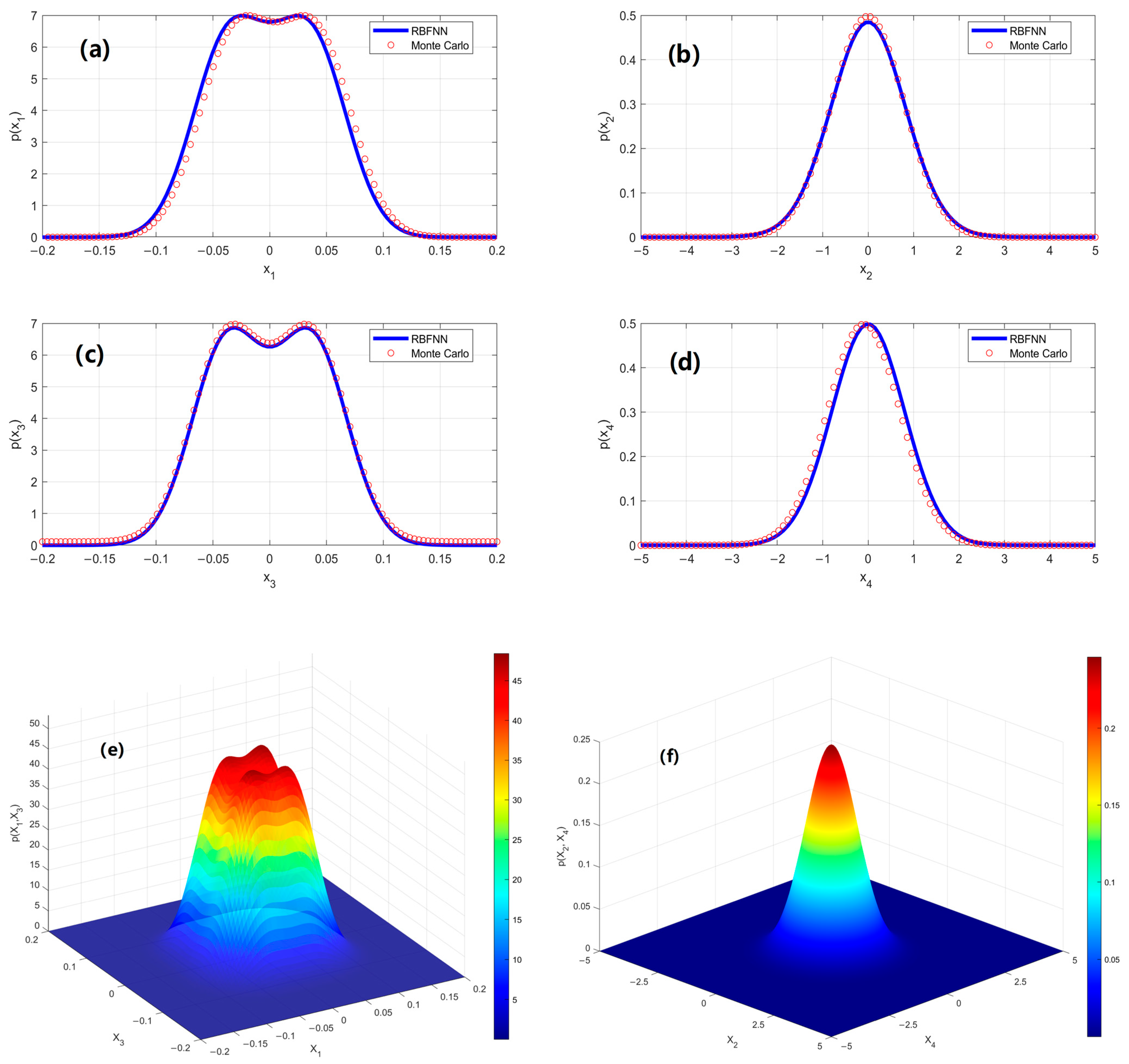
Taking the suspended cable characteristics of the Pearl River Huangpu Bridge from Section 2.4 as a case study, determine the probability density function (PDF) of the steady-state response of the suspended cables under specified damage conditions. All figures compare the results obtained from GRBFNN with those from the Monte Carlo simulation (MCS). The two sets of results show excellent agreement, demonstrating the accuracy and applicability of the GRBFNN method for such problems.

In Figure 4, subplots (a) and (c) show unimodal symmetric distributions for the displacement PDFs, resembling Gaussian distributions but with higher kurtosis, indicating that system responses tend to concentrate near the mean under damage conditions. Specifically, the peak of the in-plane displacement in Figure 4a is located near zero, while the out-of-plane displacement in Figure 4c exhibits a noticeably wider range, suggesting greater variability, which may be closely associated with a reduction in out-of-plane stiffness due to damage. Figure 4b,d present the velocity PDFs, both of which approximate standard normal distributions. However, the in-plane velocity shows a sharper and taller peak, indicating a more stable response. In contrast, the out-of-plane velocity distribution is flatter, suggesting it is more affected by damage and exhibits increased randomness. Figure 4e shows the joint PDF of in-plane and out-of-plane displacements, which exhibits a saddle-shaped distribution, indicating a certain degree of negative correlation. This may result from coupling effects induced by damage, such as the suppression of out-of-plane responses by in-plane vibrations. In contrast, the joint PDF of velocities in Figure 4f appears nearly circular, suggesting weak correlation between in-plane and out-of-plane velocities and indicating that their responses are approximately independent.

Figure 4. The stationary response of PDFs of the cable system under the specified damage conditions: (a) the marginal PDFs p(X₁) of in-plane displacement; (b) the marginal PDFs $p\left(X_2\right)$ of in-plane velocity; (c) the marginal PDFs $p\left(X_3\right)$ of out-of-plane displacement; (d) the marginal PDFs $p\left(X_4\right)$ of out-of-plane velocity; (e) the joint PDFs $p(X_1,X_3)$ of in-plane and out-of-plane displacement; (f) the joint PDFs $p(X_2,X_4)$ of in-plane and out-of-plane velocity. The parameters of this system are $\alpha$ = 0.4, $\delta$ = 0.2, $\eta$ = 0.3, D1 = D2 = 0.02 (Lines: GRBFNN solutions, Symbols: MCS results).

Figure 4. The stationary response of PDFs of the cable system under the specified damage conditions: (a) the marginal PDFs p(X₁) of in-plane displacement; (b) the marginal PDFs $p\left(X_2\right)$ of in-plane velocity; (c) the marginal PDFs $p\left(X_3\right)$ of out-of-plane displacement; (d) the marginal PDFs $p\left(X_4\right)$ of out-of-plane velocity; (e) the joint PDFs $p(X_1,X_3)$ of in-plane and out-of-plane displacement; (f) the joint PDFs $p(X_2,X_4)$ of in-plane and out-of-plane velocity. The parameters of this system are $\alpha$ = 0.4, $\delta$ = 0.2, $\eta$ = 0.3, D1 = D2 = 0.02 (Lines: GRBFNN solutions, Symbols: MCS results).

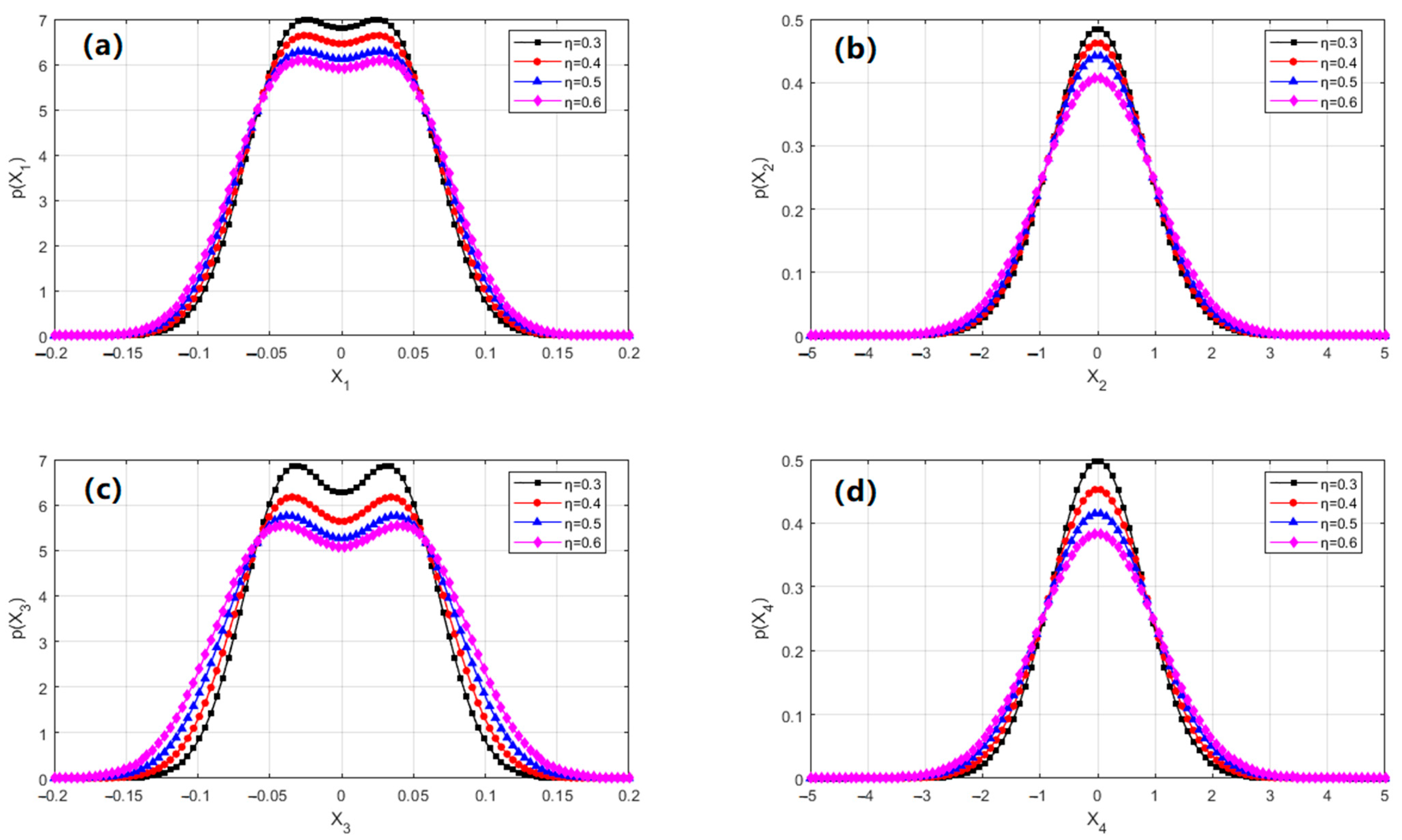
Figure 5 analyzes the effect of the damage severity parameter η on the system’s steady-state probability density functions. Figure 5a,c reveal that as η increases (i.e., as the severity of damage intensifies), the distributions of displacement $p\left(X_1\right)$ and $p\left(X_3\right)$ broaden significantly, and their peak values decrease. For instance, when η increases from 0.1 to 0.5, the peak of $p\left(X_1\right)$ decreases by approximately 30%, and the distribution tails become heavier, indicating a marked increase in uncertainty of the displacement response. The broadening of the out-of-plane displacement $p\left(X_3\right)$ is even more pronounced, suggesting greater sensitivity to the severity of damage. The velocity PDFs shown in Figure 5b,d, namely $p\left(X_2\right)$ and $p\left(X_4\right)$, also broaden with increasing η, but to a lesser extent than the displacement variables. Notably, the kurtosis of $p\left(X_4\right)$ decreases more rapidly, and its overall distribution tends to approach uniformity.

Figure 5. The changes of the stationary probability functions with different damage severity parameters: (a) the marginal PDFs p(X₁) of in-plane displacement; (b) the marginal PDFs $p\left(X_2\right)$ of in-plane velocity; (c) the marginal PDFs $p\left(X_3\right)$ of out-of-plane displacement; (d) the marginal PDFs $p\left(X_4\right)$ of out-of-plane velocity. The parameters of this system are $\alpha$ = 0.4, $\delta$ = 0.2, D1 = D2 = 0.02 (Lines: GRBFNN solutions, Symbols: MCS results).

Figure 5. The changes of the stationary probability functions with different damage severity parameters: (a) the marginal PDFs p(X₁) of in-plane displacement; (b) the marginal PDFs $p\left(X_2\right)$ of in-plane velocity; (c) the marginal PDFs $p\left(X_3\right)$ of out-of-plane displacement; (d) the marginal PDFs $p\left(X_4\right)$ of out-of-plane velocity. The parameters of this system are $\alpha$ = 0.4, $\delta$ = 0.2, D1 = D2 = 0.02 (Lines: GRBFNN solutions, Symbols: MCS results).

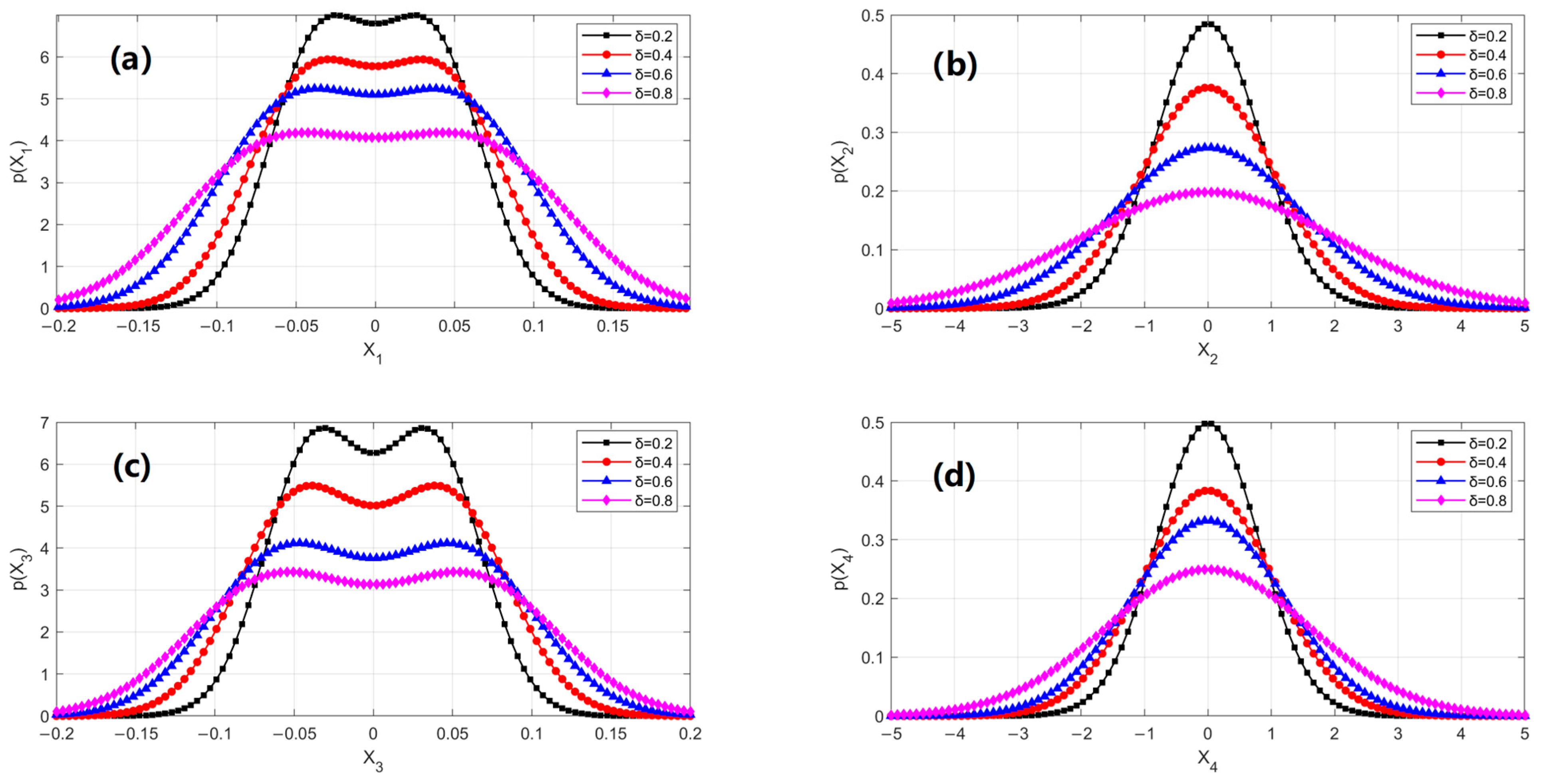
Figure 6 investigates the effect of the damage range parameter δ on the PDFs. Overall, when δ exceeds 0.3, the marginal distributions generally exhibit noticeable positive skewness, indicating an increased probability of large-magnitude displacements. As δ increases, the symmetry of all distributions is preserved, but their peak values steadily decline. This behavior results from a wider damage range causing stiffness degradation over a larger portion of the cable, which in turn amplifies geometric nonlinearity in the out-of-plane response. Meanwhile, the mean of the in-plane displacement shifts due to changes in the mass distribution of the damaged region, which alters the system’s static equilibrium position.

Figure 6. The changes of the stationary probability functions with different damage extent parameters: (a) the marginal PDFs p(X₁) of in-plane displacement; (b) the marginal PDFs $p\left(X_2\right)$ of in-plane velocity; (c) the marginal PDFs $p\left(X_3\right)$ of out-of-plane displacement; (d) the marginal PDFs $p\left(X_4\right)$ of out-of-plane velocity. The parameters of this system are $\alpha$ = 0.4, $\eta$ = 0.3, D1 = D2 = 0.02 (Lines: GRBFNN solutions, Symbols: MCS results).

Figure 6. The changes of the stationary probability functions with different damage extent parameters: (a) the marginal PDFs p(X₁) of in-plane displacement; (b) the marginal PDFs $p\left(X_2\right)$ of in-plane velocity; (c) the marginal PDFs $p\left(X_3\right)$ of out-of-plane displacement; (d) the marginal PDFs $p\left(X_4\right)$ of out-of-plane velocity. The parameters of this system are $\alpha$ = 0.4, $\eta$ = 0.3, D1 = D2 = 0.02 (Lines: GRBFNN solutions, Symbols: MCS results).

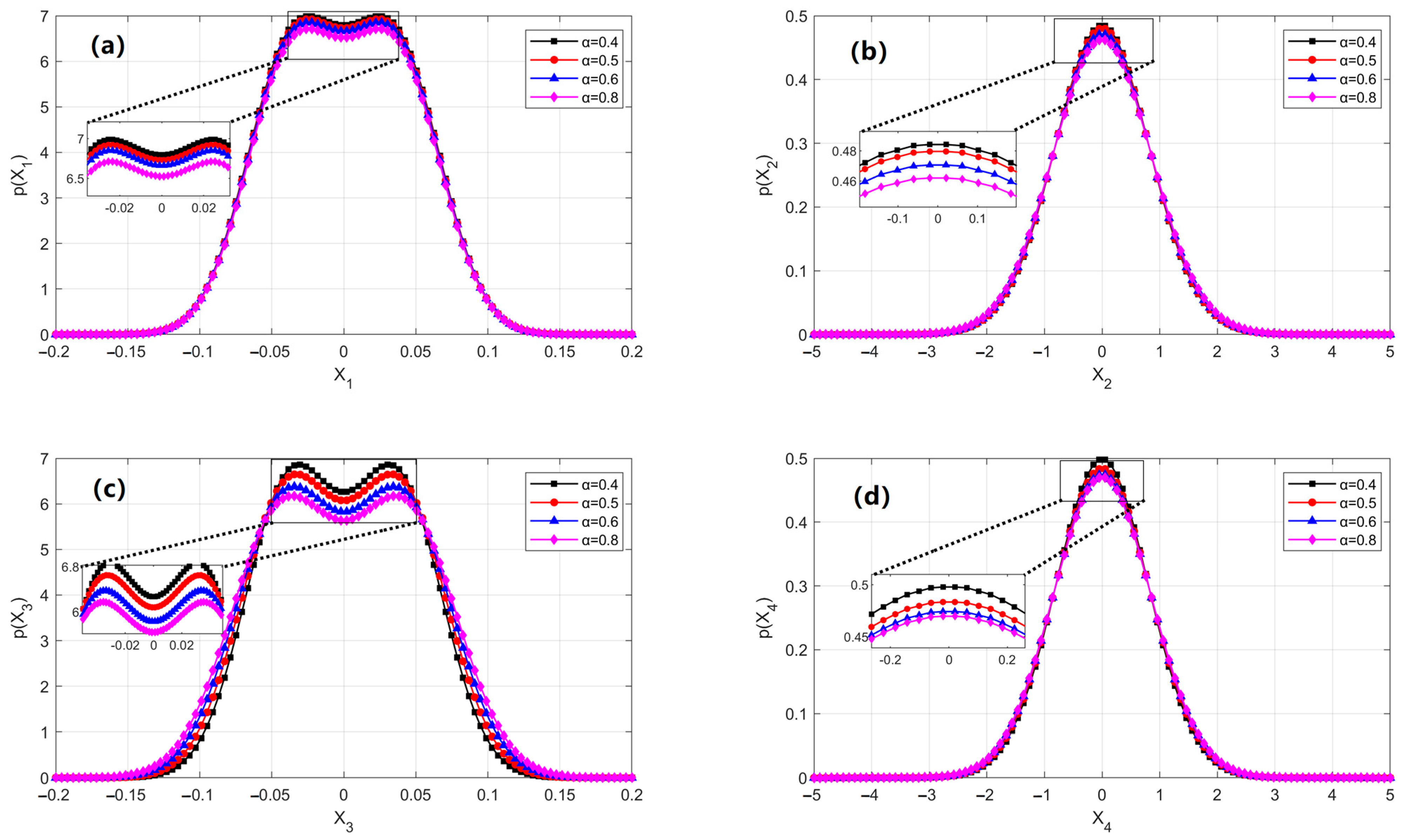
Figure 7 further demonstrates the influence of the damage location parameter α on the marginal PDFs of displacement. Figure 7b,d show that changes in damage location cause only minor variations in the marginal PDFs, indicating that velocity variables are relatively insensitive to damage location. However, in Figure 7c, the out-of-plane displacement PDF exhibits a more complex multimodal distribution when the damage is located at the mid-span of the cable. This suggests that central damage more readily excites coupled responses among higher-order vibration modes. In contrast, when the damage is near the boundaries, its influence on the overall response is relatively limited.

Figure 7. The changes of the stationary probability functions with different damage location parameters: (a) the marginal PDFs $p\left(X_1\right)$ of in-plane displacement; (b) the marginal PDFs $p\left(X_2\right)$ of in-plane velocity; (c) the marginal PDFs $p\left(X_3\right)$ of out-of-plane displacement; (d) the marginal PDFs $p\left(X_4\right)$ of out-of-plane velocity. The parameters of this system are $\delta$ = 0.2, $\eta$ = 0.3, D1 = D2 = 0.02 (Lines: GRBFNN solutions, Symbols: MCS results).

Figure 7. The changes of the stationary probability functions with different damage location parameters: (a) the marginal PDFs $p\left(X_1\right)$ of in-plane displacement; (b) the marginal PDFs $p\left(X_2\right)$ of in-plane velocity; (c) the marginal PDFs $p\left(X_3\right)$ of out-of-plane displacement; (d) the marginal PDFs $p\left(X_4\right)$ of out-of-plane velocity. The parameters of this system are $\delta$ = 0.2, $\eta$ = 0.3, D1 = D2 = 0.02 (Lines: GRBFNN solutions, Symbols: MCS results).

4.2. Reliability Analysis by GRBFNN and SORM

Although, from a strictly mathematical perspective, solving Equation (49) requires preserving the degrees of freedom in the state space, fixing the state variables and studying the time evolution of the density function $R\left(t\right)$ can be fully justified under certain conditions in practical applications. This approach can be regarded as a form of local reliability response analysis, commonly used to assess the time-varying failure risk of the system near critical state points, especially when these points lie close to the limit-state boundary or represent significant operating conditions. Therefore, due to the complexity of solving multi-variable differential Equation (49), the method of fixing state variables, while not capable of directly providing the overall failure probability, can still offer valuable pointwise information, boundary conditions, and model validation references for global analysis, making it practically meaningful and operationally feasible [34].

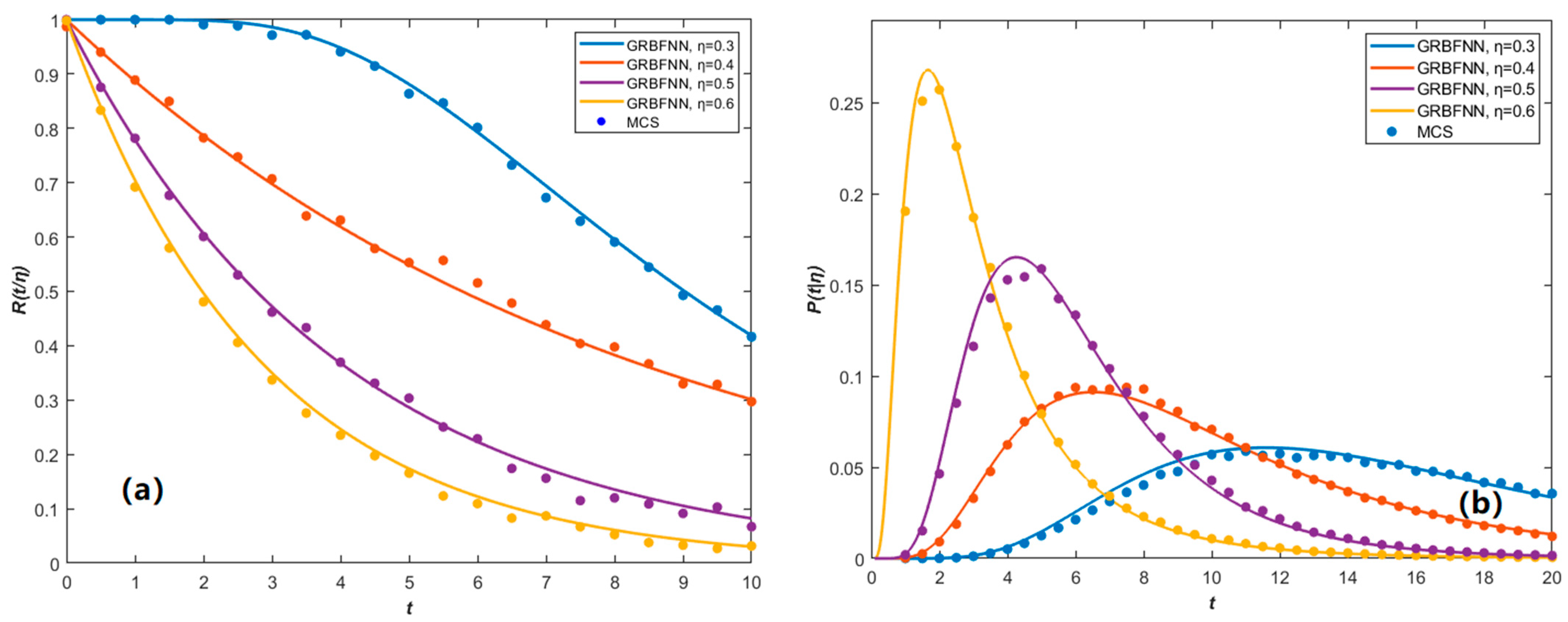
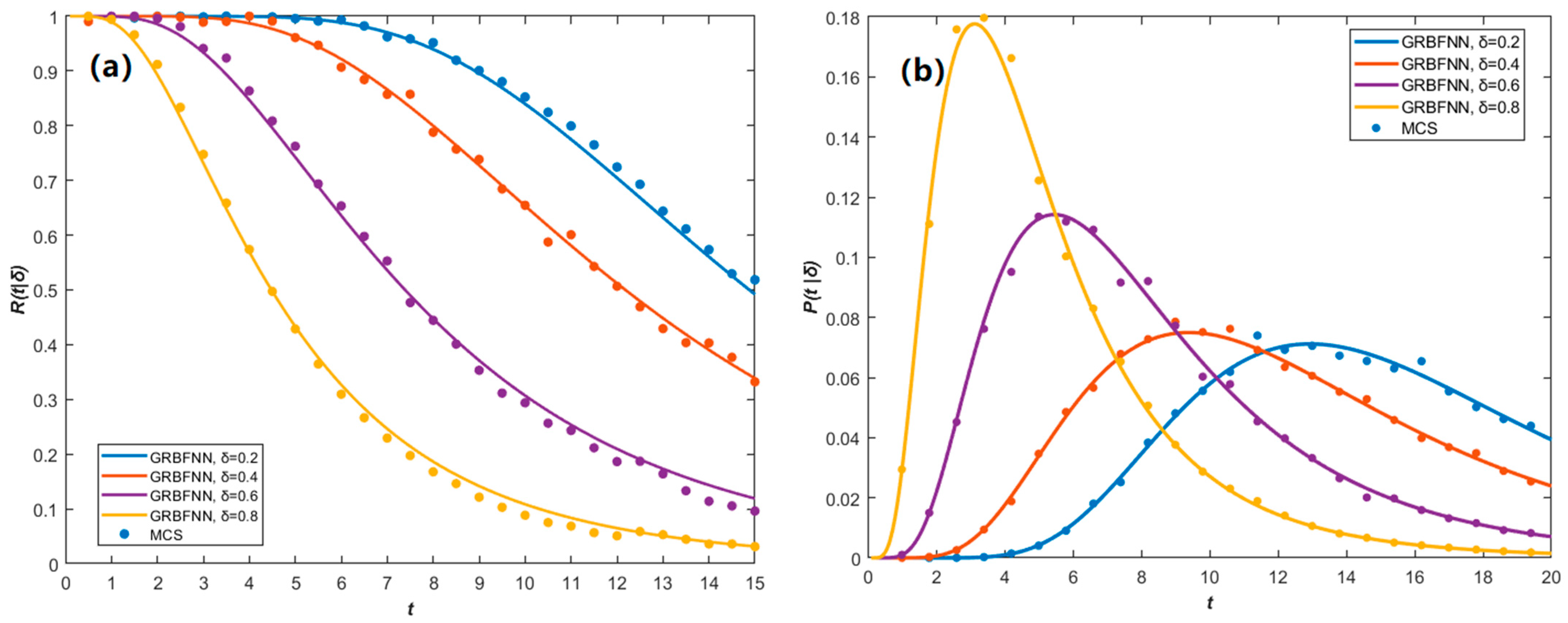
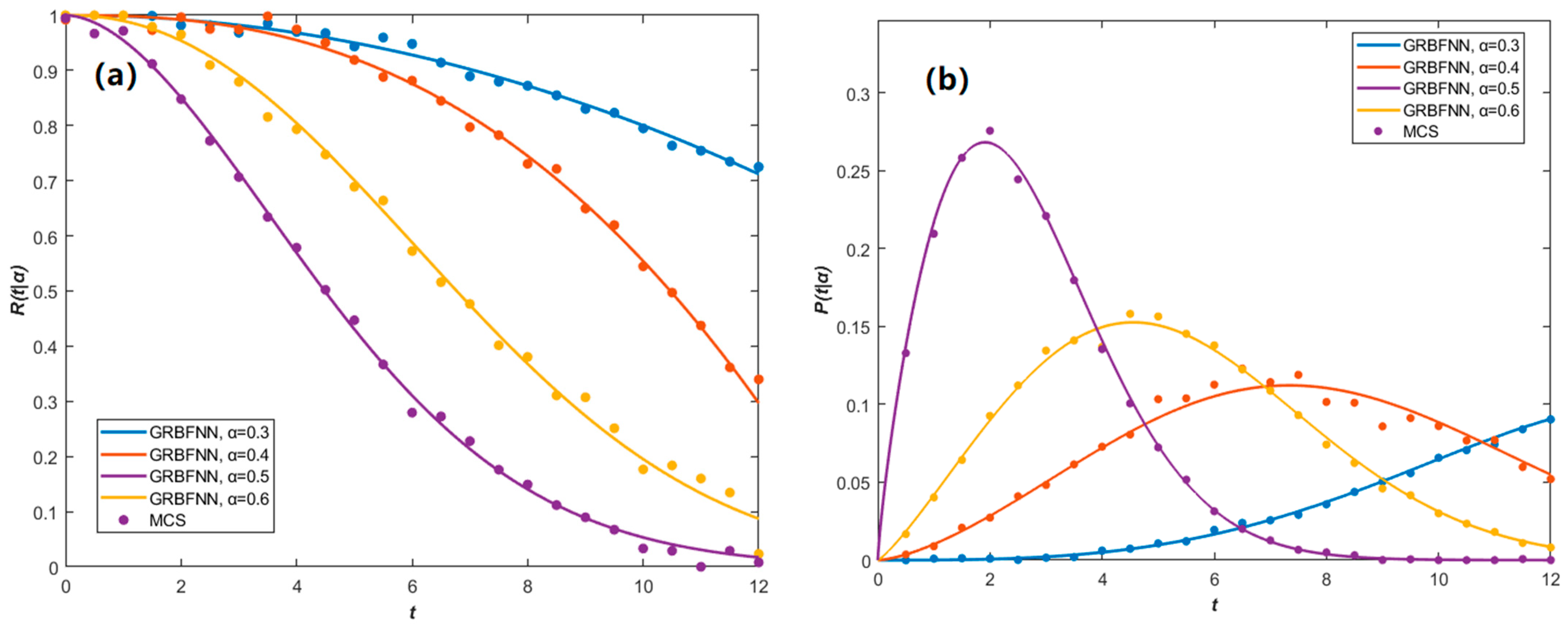
Therefore, in order to systematically investigate the influence of individual damage characteristics on the structural reliability of suspended cables, a series of time-dependent reliability functions and the corresponding first-passage probability were constructed by varying one damage parameter at a time while keeping the others fixed. In Figure 8, Figure 9 and Figure 10, GRBFNN predictions are compared with those from MCS outcomes. The consistency observed between them highlights the capability of GRBFNN to accurately model the problem under consideration.

As shown in Figure 8, an increase in η leads to a faster decay of reliability and a significant rise in the probability of the structure exceeding the safety threshold within a shorter period. Furthermore, a comprehensive comparison among Figure 8 and Figure 10 indicates that η is the most sensitive parameter driving structural failure.

As illustrated in Figure 9, with an increase in δ, the reliability lifetime of the suspended cable is shortened, and the early failure probability increases, suggesting that large-scale damage accelerates structural degradation. This implies that even with η held constant, expanding δ can still markedly reduce structural reliability [35].

According to Figure 10a, reliability is lowest when the damage is located near the mid-span, likely due to this region being a high-stress zone where damage causes the most critical effects. Figure 10b shows that failure risk decreases as the damage location shifts away from the center, consistent with the observation in Figure 7.

These reliability analysis results indicate that the higher η or larger δ directly undermine the load-bearing capacity of the structure, while α amplifies the effect of damage through its positional influence. In structural health monitoring systems, it is therefore essential to prioritize the detection of regions with high η and deploy sensors at sensitive locations such as the central segment of the suspended cable.

In addition to the above reliability analysis, failure probability calculation is essential in engineering but often intractable due to complex, high-dimensional integrals. Direct integration is computationally prohibitive, and while Monte Carlo methods are versatile, they require extensive sampling for rare events, leading to low efficiency.

The First-Order Reliability Method (FORM) and Second-Order Reliability Method (SORM) provide efficient approximate analysis approaches to address these challenges. FORM transforms the failure probability calculation into a geometric problem in standard normal space by linearizing the limit state function at the most probable failure point, while SORM enhances accuracy through second-order corrections that account for the curvature of the limit state surface. Both methods maintain high computational efficiency while delivering sufficient accuracy for reliability assessment in engineering problems [36].

The foundation of structural reliability analysis is the establishment of appropriate limit state functions (LSFs) that can accurately describe the transition boundary from safe states to failure states. Considering the dynamic response characteristics of cable suspension structures under random loading, this study establishes the limit state function as

$$g\left(\mathit{X}\right)={\delta }_{\mathrm{limit}}-{\delta }_{\mathrm{response}}\left(\mathit{X}\right)$$

(63)

where the physical meanings of the parameters are defined as follows: ${\delta }_{\mathrm{limit}}$ represents the maximum allowable displacement limit for structural design, typically determined by relevant codes or engineering experience, while ${\delta }_{\mathrm{response}}\left(\mathit{X}\right)$ denotes the actual displacement response of the structure under the action of random variable vector $\mathit{X}$. The system state variable vector $\mathit{X}=[X_1,X_2,X_3,X_4{]}^T$. When $g\left(\mathbf{X}\right)\le 0$, the structure is considered to have failed.

The structural failure probability is defined as the probability that the random variable vector $\mathit{X}$ falls within the failure domain, with its mathematical expression given by

$$P_f=P\left[g\left(\mathit{X}\right)\le 0\right]={{\displaystyle \int }}_{g\left(X\right)\le 0}{f}_X\left(x\right)dx$$

(64)

As we know from above, $f_{\mathit{X}}\left(\mathbf{x}\right)$ was obtained by GRBFNN, whose mathematical expression can be represented as

$$f_X\left(x\right)={\displaystyle \sum }_{j=1}^{N_G}{w}_j\left(t\right)\hspace{0.17em}{G}_j\left(x;{\mathsf{\mu }}_j,{\Sigma }_j\right)$$

(65)

Therefore, the complete expression for failure probability becomes

$$P_f={\displaystyle \sum }_{j=1}^{N_G}{w}_j\left(t\right){{\displaystyle \int }}_{g\left(x\right)\le 0}{G}_j\left(x;{\mathsf{\mu }}_j,{\Sigma }_j\right)dx$$

(66)

The core principle of FORM involves performing first-order Taylor expansion of the limit state function at the most probable failure point (design point), transforming the complex reliability integral problem into a geometric problem in standard normal space through linearization treatment [36]. To perform reliability calculations in standard normal space, it is necessary to map random variables $\mathit{X}$ in physical space to variables $\mathit{U}$ in standard normal space. This transformation must preserve probability measures, ensuring that

$$P\left[\mathit{X}\in D\right]=P\left[\mathit{U}\in T\left(D\right)\right]$$

(67)

where $T(\cdot )$ represents the transformation operator, and $D$ denotes any region in physical space. For non-normal distributions with known joint distributions, the Rosenblatt transformation is adopted:

$${\mathit{U}}_i={\Phi }^{-1}\left(F_{X_i\mid X_1,\dots ,X_{i-1}}\left(x_i\mid x_1,\dots ,x_{i-1}\right)\right),i=1,2,3,4$$

(68)

where $F_{X_i\mid X_1,\dots ,X_{i-1}}(\cdot )$ represents the conditional cumulative distribution function of the $i$-th state variable, and ${\Phi }^{-1}(\cdot )$ denotes the inverse cumulative distribution function of the standard normal distribution. The Rosenblatt transformation can handle arbitrary forms of joint distributions but requires complete conditional distribution information.

In standard normal space, the failure probability calculation problem transforms to

$$P_f=P\left[g\left(\mathit{X}\right)\le 0\left]=P\right[G\left(\mathit{U}\right)\le 0\right]={{\displaystyle \int }}_{G\left(\mathit{U}\right)\le 0}{\varphi }_n\left(\mathit{u}\right)d\mathit{u}$$

(69)

where $G\left(\mathit{U}\right)=g\left[T^{-1}\left(\mathit{U}\right)\right]$ represents the limit state function in standard normal space, and ${\varphi }_n\left(\mathit{u}\right)={\displaystyle \frac{1}{(2\pi {)}^{n/2}}}\mathrm{e}\mathrm{x}\mathrm{p}\left(-{\displaystyle \frac{1}{2}}{\mathit{u}}^T\mathit{u}\right)$ denotes the n-dimensional standard normal distribution density function. The design point ${\mathit{u}}^{\mathrm{*}}$ is defined as the closest point to the origin on the limit state surface $G\left(\mathit{U}\right)=0$, determined by solving the following constrained optimization problem:

$${\mathit{u}}^{*}=\arg \underset{u}{\min }{\displaystyle \frac{1}{2}}{\mathit{u}}^T\mathit{u} subject to G\left(\mathit{u}\right)=0$$

(70)

which can be solved by the Lagrange Multiplier Method; finally, we obtain ${\mathit{u}}^{*}=-\lambda \nabla G\left({\mathit{u}}^{*}\right)$. This indicates that the design point lies along the direction of the line connecting the origin to the tangent point of the limit state surface. Therefore, the reliability index $\beta$ is defined as the Euclidean distance from the design point to the origin, and the structural failure probability can be expressed as Equation (72),

$$\beta = \parallel {\mathit{u}}^{*}\parallel$$

(71)

$$P_f^{\mathrm{FORM}}=\Phi \left(-\beta \right)$$

(72)

where $\Phi (\cdot )$ represents the cumulative distribution function of the standard normal distribution.

The Second-Order Reliability Method (SORM) represents a high-precision reliability analysis method developed based on FORM. By considering curvature information of the limit state surface, SORM performs second-order correction to the linearization approximation of FORM, thereby significantly improving the accuracy of failure probability estimation [36]. At the design point ${\mathit{u}}^{\mathrm{*}}$, the limit state function $G\left(\mathit{U}\right)$ is expanded using second-order Taylor series:

$$G\left(\mathit{U}\right)\approx G\left({\mathit{u}}^{*}\right)+\nabla G{\left({\mathit{u}}^{*}\right)}^T\left(\mathit{U}-{\mathit{u}}^{*}\right)+{\displaystyle \frac{1}{2}}{\left(\mathit{U}-{\mathit{u}}^{*}\right)}^T\mathit{H}\left({\mathit{u}}^{*}\right)\left(\mathit{U}-{\mathit{u}}^{*}\right)$$

(73)

where gradient vector can be expressed as Equation (74), and Hessian Matrix $H\left({\mathit{u}}^{\mathrm{*}}\right)$ at the design point of $G\left(\mathit{U}\right)$ is defined as Equation (75) in order to solve our fourth-order differential equation:

$$\nabla G\left({\mathit{u}}^{*}\right)={\left[{\displaystyle \frac{\partial G}{\partial U_1}},{\displaystyle \frac{\partial G}{\partial U_2}},{\displaystyle \frac{\partial G}{\partial U_3}},{\displaystyle \frac{\partial G}{\partial U_4}}\right]}_{\mathit{u}={\mathit{u}}^{*}}^T$$

(74)

$$H\left(u^{*}\right)={\left[\begin{array}{cccc}{\displaystyle \frac{{\partial }^{2}G}{\partial U_1^2}}& {\displaystyle \frac{{\partial }^{2}G}{\partial U_1\partial U_2}}& {\displaystyle \frac{{\partial }^{2}G}{\partial U_1\partial U_3}}& {\displaystyle \frac{{\partial }^{2}G}{\partial U_1\partial U_4}}\\ {\displaystyle \frac{{\partial }^{2}G}{\partial U_2\partial U_1}}& {\displaystyle \frac{{\partial }^{2}G}{\partial U_2^2}}& {\displaystyle \frac{{\partial }^{2}G}{\partial U_2\partial U_3}}& {\displaystyle \frac{{\partial }^{2}G}{\partial U_2\partial U_4}}\\ {\displaystyle \frac{{\partial }^{2}G}{\partial U_3\partial U_1}}& {\displaystyle \frac{{\partial }^{2}G}{\partial U_3\partial U_2}}& {\displaystyle \frac{{\partial }^{2}G}{\partial U_3^2}}& {\displaystyle \frac{{\partial }^{2}G}{\partial U_3\partial U_4}}\\ {\displaystyle \frac{{\partial }^{2}G}{\partial U_4\partial U_1}}& {\displaystyle \frac{{\partial }^{2}G}{\partial U_4\partial U_2}}& {\displaystyle \frac{{\partial }^{2}G}{\partial U_4\partial U_3}}& {\displaystyle \frac{{\partial }^{2}G}{\partial U_4^2}}\end{array}\right]}_{u=u^{*}}$$

(75)

Afterwards, we are supposed to calculate the principal curvature, as these quantities directly characterize the local geometric properties of the limit state surface in the vicinity of the design point. The initial step in the principal curvature calculation is Hessian matrix normalization:

$${\mathit{H}}_{\mathrm{norm}}={\displaystyle \frac{\mathit{H}\left({\mathit{u}}^{*}\right)}{\parallel \nabla G\left({\mathit{u}}^{*}\right)\parallel }}$$

(76)

To extract principal curvatures, the coordinate system is rotated so that one axis aligns with the normal direction of the limit state surface at the design point. This is achieved by constructing an orthogonal rotation matrix that aligns the gradient direction with a principal axis. The unit normal vector at the design point is defined as

$$\mathit{\alpha }=-{\displaystyle \frac{\nabla G\left({\mathit{u}}^{*}\right)}{\parallel \nabla G\left({\mathit{u}}^{*}\right)\parallel }}$$

(77)

The negative sign ensures that the normal vector points toward the safe domain, consistent with the conventional definition of the reliability index. The rotation matrix $\mathit{R}$ is then constructed to satisfy the constraint:

$$\mathit{R}\mathbf{\alpha }={[0,0,0,1]}^T$$

(78)

The rotated Hessian matrix is subsequently obtained through the similarity transformation:

$${\mathit{H}}_{\mathrm{rot}}={\mathit{R}}^T{\mathit{H}}_{\mathrm{norm}}\mathit{R}$$

(79)

Following the coordinate transformation, the principal curvatures are extracted from the upper-left submatrix of the rotated Hessian, which contains the curvature information in the tangential directions to the limit state surface [36]. This submatrix is denoted as

$$\mathit{B}={\mathit{H}}_{\mathrm{rot}}\left(1:3,1:3\right)$$

(80)

where B represents the reduced Hessian matrix in the tangential space. The principal curvatures ${\kappa }_i$ for $i=1,2,3$ are determined as the eigenvalues of this matrix through the characteristic equation

$$det\left(\mathit{B}-\kappa \mathit{I}\right)=0$$

(81)

Consequently, the corrected failure probability is calculated by using the Breitung formula as Equation (82),

$$P_f\approx \Phi \left(-\beta \right){\displaystyle \prod }_{i=1}^3{\displaystyle \frac{1}{\sqrt{1+\beta {\kappa }_i}}}$$

(82)

where $\beta =\parallel u^{\mathrm{*}}\parallel$ is the FORM reliability index.

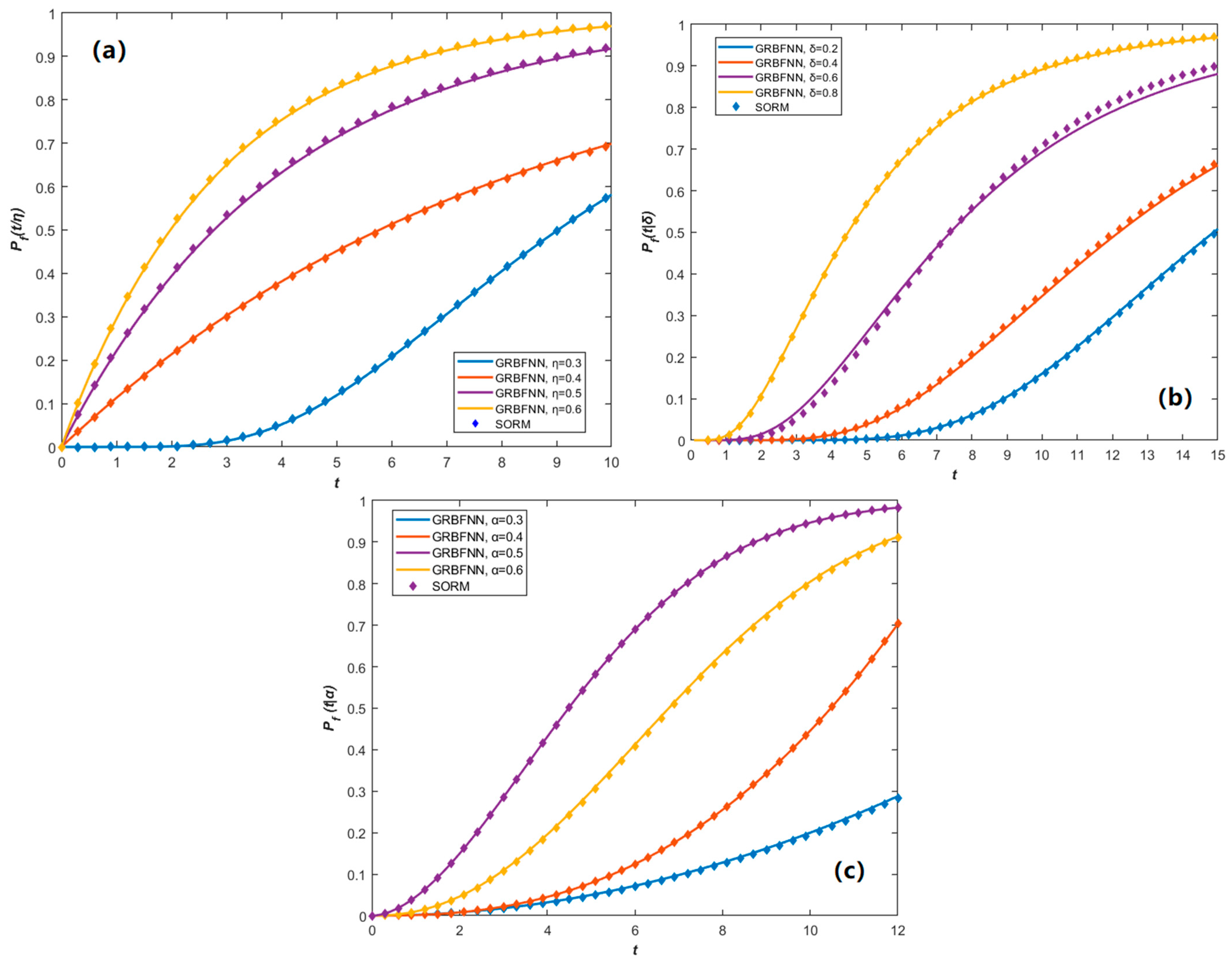
A comparative analysis between GRBFNN and SORM in Figure 11 reveals the time-dependent behavior of failure probability under different parameter settings. Parameters η and δ mainly influence its growth magnitude, while α affects the critical transition point due to its positional sensitivity. GRBFNN closely matches SORM results in most cases and demonstrates higher accuracy in strongly nonlinear regimes, offering valuable theoretical support for damage-tolerant design. However, it is important to note that the current modeling framework assumes time-invariant system parameters and stationary Gaussian excitation. While this assumption is suitable for steady-state reliability analysis, it does not capture time-dependent behaviors such as evolving damage, stiffness degradation, or non-stationary inputs.

5. Conclusions

This study proposed an integrated framework that combines nonlinear stochastic vibration analysis with reliability evaluation to systematically investigate the dynamic behavior and failure probability of damaged cable structures under random excitations. The main findings and contributions are summarized as follows:

• Static Modeling and Validation: A static mathematical model incorporating damage parameters was developed, and the analytical solution for cable sag was derived. Using the Pearl River Huangpu Bridge as a case study, the accuracy of the analytical solution was validated by the finite difference method (FDM). The relative errors remained below 5% across the entire span, demonstrating the model’s reliability and practical applicability.
• Stochastic Dynamic Modeling: A coupled nonlinear stochastic dynamic model was established for in-plane and out-of-plane vibrations with Gaussian white noise excitation. Damage-induced interactions were captured, and the governing equations were reduced through Galerkin discretization, enabling efficient numerical analysis.
• GRBFNN-Based Solution to FPK Equation: To address the challenge of solving high-dimensional, nonlinear stochastic systems, a numerical scheme based on the Gaussian Radial Basis Function Neural Network (GRBFNN) was introduced to approximate the solution of the Fokker–Planck–Kolmogorov (FPK) equation. The GRBFNN results showed excellent agreement with Monte Carlo simulations under various damage scenarios, confirming its accuracy and computational efficiency.
• Reliability Assessment and Sensitivity Analysis: Based on the probability density functions from GRBFNN, structural reliability indices and failure probabilities were evaluated using FORM and SORM. Results indicate that damage severity (η) is the dominant factor affecting reliability, while damage extent (δ) significantly reduces structural lifespan. Damage location (α) influences failure evolution by activating higher-order modes, with the highest risk near the midspan—highlighting the need for focused monitoring in this region.

In summary, this study presents a unified theoretical framework integrating static analysis, stochastic dynamic modeling, probabilistic density approximation, and reliability evaluation. It offers a scientific basis for damage diagnosis and lifetime prediction of suspension systems, providing engineering insights into the design and maintenance of large-scale flexible structures.

Future research will aim to enhance the realism and applicability of the proposed framework by incorporating material nonlinearity, multi-physical coupling effects, and experimental validation through scaled physical models or engineering collaborations. In parallel, future efforts will focus on extending the framework to non-stationary responses, incorporating time-dependent damage evolution and environmental effects to improve practical relevance in long-term monitoring.

References

1. Sloane, D.J.M.; Betti, R.; Marconi, G. Experimental analysis of a nondestructive corrosion monitoring system for main cables of suspension bridges. J. Bridge Eng. 2013, 18, 653–662. [Google Scholar] [CrossRef]
2. Feng, J.; Gao, K.; Gao, W.; Liao, Y.; Wu, G. Machine learning-based bridge cable damage detection under stochastic effects of corrosion and fire. Eng. Struct. 2022, 264, 114421. [Google Scholar] [CrossRef]
3. Morgado, T.L.M.; Sousa e Brito, A. A failure analysis study of a prestressed steel cable of a suspension bridge. Case Stud. Constr. Mater. 2015, 3, 40–47. [Google Scholar] [CrossRef]
4. Li, D.; Ou, J.; Lan, C.; Li, H. Monitoring and failure analysis of corroded bridge cables under fatigue loading using acoustic emission sensors. Sensors 2012, 12, 3901–3915. [Google Scholar] [CrossRef]
5. Gao, W.; Zhang, N.; Ji, J. A new method for random vibration analysis of stochastic truss structures. Finite Elem. Anal. Des. 2009, 45, 190–199. [Google Scholar] [CrossRef]
6. Larsen, A.; Larose, G.L. Dynamic wind effects on suspension and cable-stayed bridges. J. Sound Vib. 2015, 334, 2–28. [Google Scholar] [CrossRef]
7. Sun, L.; Chen, L.; Huang, H. Stay cable vibration mitigation: A review. Adv. Struct. Eng. 2022, 25, 3368–3404. [Google Scholar] [CrossRef]
8. Lan, L.; Chen, L.; Zhao, Y. Nonlinear random vibration of damaged cable systems under Gaussian white noise excitations. Nonlinear Dyn. 2025, 113, 4015–4029. [Google Scholar] [CrossRef]
9. He, T.; Li, B.; Yang, J.; Xia, Y.; Qian, J. Theoretical research on suspension bridge cable damage assessment based on vehicle-induced cable force. Buildings 2024, 14, 3962. [Google Scholar] [CrossRef]
10. Xu, Y.; Zhang, J.; Li, J.; Wang, S. Damage identification of long-span bridges using the hybrid of convolutional neural network and long short-term memory network. Algorithms 2021, 14, 180. [Google Scholar] [CrossRef]
11. Dang, H.V.; Raza, M.; Nguyen, T.V.; Bui-Tien, T.; Nguyen, H.X. Damage detection and localization in a cable stayed bridge using a hybrid deep learning approach. Eng. Struct. 2021, 237, 112417. [Google Scholar] [CrossRef]
12. Pathirage, C.S.N.; Li, J.; Li, L.; Hao, H.; Liu, W.; Wang, R. Structural damage identification based on autoencoder neural networks and deep learning. Eng. Struct. 2018, 172, 13–28. [Google Scholar] [CrossRef]
13. Wang, Z.; Cha, Y.J. Unsupervised deep learning approach using a deep auto-encoder with a one-class support vector machine to detect structural damage. Struct. Health Monit. 2021, 20, 406–425. [Google Scholar] [CrossRef]
14. Sony, S.; Laventure, S.; Sadhu, A. A literature review of next-generation smart sensing technology in structural health monitoring. Struct. Control Health Monit. 2019, 26, e2321. [Google Scholar] [CrossRef]
15. Lin, Y.Z.; Nie, Z.H.; Ma, H.W. Structural damage detection with automatic feature-extraction through deep learning. Comput. -Aided Civ. Infrastruct. Eng. 2017, 32, 1025–1046. [Google Scholar] [CrossRef]
16. Li, S.; Wei, S.; Bao, Y.; Li, H. Condition assessment of cables by pattern recognition of vehicle-induced cable tension ratio. Eng. Struct. 2021, 155, 1–15. [Google Scholar] [CrossRef]
17. Wang, B.; He, Z.; Zhou, Y. Time-variant reliability assessment for multiple corrosion defects of pipeline. Process Saf. Environ. Prot. 2021, 144, 156–167. [Google Scholar] [CrossRef]
18. Ou, J.; Li, H. Structural health monitoring in mainland China: Review and future trends. Struct. Health Monit. 2010, 9, 219–231. [Google Scholar] [CrossRef]
19. Chan, T.H.; Yu, L.; Tam, H.Y.; Ni, Y.Q.; Liu, S.Y.; Chung, W.H.; Cheng, L.K. Fiber Bragg grating sensors for structural health monitoring of Tsing Ma bridge: Background and experimental observation. Eng. Struct. 2006, 28, 648–659. [Google Scholar] [CrossRef]
20. Ye, X.W.; Su, Y.H.; Han, J.P. Structural health monitoring of civil infrastructure using optical fiber sensing technology: A comprehensive review. Sci. World J. 2014, 2014, 652329. [Google Scholar] [CrossRef]
21. Abdulkarem, M.; Samsudin, K.; Rokhani, F.Z.; Rasid, M.F.A. Wireless sensor network for structural health monitoring: A contemporary review of technologies, challenges, and future direction. Struct. Health Monit. 2020, 19, 693–735. [Google Scholar] [CrossRef]
22. Xiong, C.; Lu, H.; Zhu, J. Operational modal analysis of bridge structures with data from GNSS/accelerometer measurements. Sensors 2017, 17, 436. [Google Scholar] [CrossRef] [PubMed]
23. Koo, K.Y.; Brownjohn, J.M.; List, D.I.; Cole, R. Structural health monitoring of the Tamar suspension bridge. Struct. Control Health Monit. 2013, 20, 609–625. [Google Scholar] [CrossRef]
24. Zhang, J.; Guo, S.L.; Wu, Z.S.; Zhang, Q.Q. Structural identification and damage detection through long-gauge strain measurements. Eng. Struct. 2015, 99, 173–183. [Google Scholar] [CrossRef]
25. Ditommaso, R.; Ponzo, F.C. Identifying Damage in Structures: Definition of Thresholds to Minimize False Alarms in SHM Systems. Buildings 2024, 14, 821. [Google Scholar] [CrossRef]
26. Bouaanani, N. Numerical investigation of the modal sensitivity of suspended cables with localized damage. J. Sound Vib. 2006, 292, 1015–1030. [Google Scholar] [CrossRef]
27. Kim, H.; Kim, J. Prediction of Cable Behavior Using Finite Element Analysis Results for Flexible Cables. Sensors 2023, 23, 5707. [Google Scholar] [CrossRef]
28. Mehrabi, A.B.; Tabatabai, H. Unified finite difference formulation for free vibration of cables. J. Struct. Eng.-ASCE 1998, 124, 1313–1322. [Google Scholar] [CrossRef]
29. Recupero, A.; Longo, G.; Granata, M.F. Structural analysis of cable-stayed structures in the construction sequence of bridges built by cantilevering. Int. J. Bridge Eng. 2016, 71–96. [Google Scholar] [CrossRef]
30. Gan, Q.; Huang, Y.; Wang, R.; Rao, R. Tension estimation of hangers with shock absorber in suspension bridge using finite element method. J. Vibro-Eng. 2019, 21, 587–601. [Google Scholar] [CrossRef]
31. Zheng, P.; Zhao, Y.; Wu, X.; Chen, L. Revisited modeling and nonlinear oscillation behaviors of multi-segment damaged suspended cables in thermal environments. Meccanica 2022, 57, 1831–1851. [Google Scholar] [CrossRef]
32. Li, W.; Guan, Y.; Huang, D.; Trisovic, N. Gaussian RBFNN method for solving FPK and BK equations in stochastic dynamical system with FOPID controller. Int. J. Non-Linear Mech. 2023, 153, 104403. [Google Scholar] [CrossRef]
33. Wang, X.; Jiang, J.; Hong, L.; Sun, J.Q. Random vibration analysis with radial basis function neural networks. Int. J. Dynam. Control 2022, 10, 1385–1394. [Google Scholar] [CrossRef]
34. Strogatz, S.H. Nonlinear Dynamics and Chaos: With Applications to Physics, Biology, Chemistry, and Engineering, 3rd ed.; Chapman and Hall/CRC: Boca Raton, FL, USA, 2024. [Google Scholar] [CrossRef]
35. Guan, Y.; Li, W.; Huang, D.; Gubeljak, N. A new LBFNN algorithm to solve FPK equations for stochastic dynamical systems under Gaussian or Non-Gaussian excitation. Chaos Solitons Fractals 2023, 173, 113641. [Google Scholar] [CrossRef]
36. Hu, Z.; Du, X. Efficient reliability-based design with second order approximations. Eng. Optim. 2018, 51, 101–119. [Google Scholar] [CrossRef]
Figure 1. Integrated framework of this study.
Vibration 08 00044 g001
Figure 2. Static and dynamic structures of a damaged cable.
Vibration 08 00044 g002
Figure 3. Schematic diagram of the RBFNN general structure and Gaussian-based implementation.
Vibration 08 00044 g003
Figure 8. (a) The influences of damage severity ( η ) on the reliability functions. (b) The influences of damage severity ( η ) on the probability of the first-passage time. The parameters of this system are α = 0.4, δ = 0.2, D1 = D2 = 0.02.
Vibration 08 00044 g008
Figure 9. (a) The influences of damage extent ( δ ) on the reliability functions. (b) The influences of damage extent ( δ ) on the probability of the first-passage time. The parameters of this system are α = 0.4, η = 0.3, D1 = D2 = 0.02.
Vibration 08 00044 g009
Figure 10. (a) The influences of damage location ( α ) on the reliability functions. (b) The influences of damage location ( α ) on the probability of the first-passage time. The parameters of this system are δ = 0.2, η = 0.3, D1 = D2 = 0.02.
Vibration 08 00044 g010
Figure 11. The influences of damage parameters on the failure probability: the parameters of this system are (a) α = 0.4, δ = 0.2 (b) α = 0.4, η = 0.3 (c) δ = 0.2, η = 0.3 (Lines: GRBFNN solutions, Symbols: SORM results).
Vibration 08 00044 g011