Parameter Estimation of Nonlinear Structural Systems Using Bayesian Filtering Methods

Abstract

This paper examines the performance of Bayesian filtering system identification in the context of nonlinear structural and mechanical systems. The objective is to assess the accuracy and limitations of the four most well-established filtering-based parameter estimation methods: the extended Kalman filter, the unscented Kalman filter, the ensemble Kalman filter, and the particle filter. The four methods are applied to estimate the parameters and the response of benchmark dynamical systems used in structural mechanics, including a Duffing oscillator, a hysteretic Bouc–Wen oscillator, and a hysteretic Bouc–Wen chain system. Based on the performance, accuracy, and computational efficiency of the methods under different operating conditions, it is concluded that the unscented Kalman filter is the most effective filtering system identification method for the systems considered, with the other filters showing large estimation errors or divergence, high computational cost, and/or curse of dimensionality as the dimension of the system and the number of uncertain parameters increased.

1. Introduction

To design and evaluate the performance of structural and mechanical systems it is essential to reliably predict features of the system behavior and response characteristics. Physics-based mechanics models are typically employed to predict the response of complex large-scale structural systems, and the features of the response that can be captured by parameterized mechanics-based models depend on their functional form and the adopted parameters. Moreover, a set of parameters rather than point values might properly characterize structural behavior due to the presence of inherent modeling uncertainty, unmeasured input excitations, and/or unknown initial conditions [1].

System identification (SI) has emerged as a primary engineering analysis tool aimed at improving the predicting capability of models from measured response data [2]. SI can be defined as the inverse problem of using measurements to infer the state and parameters of models that best fit the observed data. The objective is to maximize the predicting accuracy and capabilities of a model by minimizing modeling errors and uncertainty. Applications of SI in structural and mechanical systems include structural condition assessment and management, structural damage diagnosis/prognosis, response control, improvement of computer-aided design methods, and enhancement of experimental testing techniques, among others. In the context of linear systems, an extensive number of SI algorithms have been developed over the past decades [3]. In some applications, the features of the dynamic response of the system of interest cannot be captured by a linear model. Sources of nonlinearity include nonlinear kinematic or geometric response features, nonlinear material or constitutive behavior, nonlinear boundary conditions, nonlinear modeling of energy dissipation mechanisms or devices, and modeling of actuators, among others [4]. Moreover, nonlinear behavior and phenomena can be exploited to design systems with enhanced performance and energy harvesting capabilities. Estimation of the model parameters of nonlinear systems presents an increased challenge with respect to the linear systems counterpart, in part because of the complexity of modeling nonlinear phenomena and the lack of a closed-form general input–output mapping that applies to all nonlinear systems.

SI methods can be broadly classified as deterministic or probabilistic. Deterministic methods rely on an optimization-based strategy to minimize an objective function defined as a measure of the discrepancy between measured responses and model predictions [5,6]. On the other hand, probabilistic methods use a stochastic model of the system treating the uncertain parameters as random variables and using statistical inference (frequentist or Bayesian) to estimate the parameters; in particular Bayesian methods have received significant attention due to their ability to rigorously handle a broad class of estimation problems in linear and nonlinear systems. In Bayesian SI, the information about the parameters contained in measurements is integrated using conditional probability distributions obtained using Bayes’ theorem; the estimate of the parameters and their uncertainty are encapsulated in a probability distribution conditional on the measured data [7,8,9,10].

In addition to the estimation approach adopted, SI can be performed either considering a set of response measurements (batch estimation) or in real-time with the estimation performed every time step that a new measurement is available (recursively/sequential estimation). In dynamical systems, when the estimation process is performed recursively the resulting procedure is known as filtering [11]. In the filtering setting the estimation is performed in a predictor–corrector fashion that involves a forward projection of the estimate of the response and the parameters using a model (prediction), and subsequently integrating the measurements (correction). Filtering was formalized using probabilistic methods in the context of optimal linear filtering [12]. The most celebrated method is the Kalman filter, a recursive estimation algorithm that allows for optimal estimation (unbiased, minimum variance, and minimum mean-squared error) of the state of a linear system subjected to disturbing inputs modeled as a stochastic process by combining model predictions and response measurements.

Filtering can be applied to system identification by including uncertain parameters in the state, and the resulting procedure is known as joint state-parameter estimation or augmented state estimation [13]. When the underlying system is linear including the parameters in the state results in a nonlinear estimation problem, and nonlinear filtering methods are needed; thus, the parameter estimation problem is nonlinear irrespective of the underlying dynamics being linear or nonlinear, but with significantly stronger nonlinearities in the latter case. In the Bayesian solution of the nonlinear filtering problem, a complete functional description of the conditional probability density describing the evolution of the state is needed. Despite the possibility, in theory, to compute this evolving density function, computational limitations both in algorithmic running time and storage limits prevent the Bayesian nonlinear filtering problem from being solved in closed form. Under these conditions the problem admits a wider family of sub-optimal solutions.

The first extension of linear filtering theory to nonlinear problems proposed in the literature is the extended Kalman filter (EKF), which became the de facto accepted solution to the problem for several decades. The EKF is a recursive estimation algorithm that follows from approximating nonlinear transformations of the state distribution by linearizing the nonlinear model and using the Kalman filter on the linearized model [13]. The EKF is neither an unbiased minimum variance, nor the minimum mean-squared error estimate of the state, and its two main drawbacks are the computational issues related to the propagation of the covariance matrix, and errors resulting from the linearization performed where high-order nonlinear terms are neglected. The result is a loss of accuracy and potential filter divergence. The EKF also requires determining the Jacobian of the model, a task that is generally computationally intensive.

To overcome the main limitations of the EKF, recent efforts have focused on the development of more advanced nonlinear filtering methods that show improved performance. The three most well-established new methods are the unscented Kalman filter (UKF) [14], the ensemble Kalman filter (EnKF) [15], and the particle filter (PF) [16]. The Kalman filtering-based nonlinear methods approximate the distributions involved as Gaussian, with their mean and covariance estimated using a deterministic sample (for the UKF) or a random sample (for the EnKF). On the other hand, particle filters use a random sample to directly approximate the filtering distribution by a probability mass function. This implies that Kalman filtering methods are suitable only when the distributions involved are unimodal, while particle filters can handle distributions with non-Gaussian features, such as high skewness, heavy tails, or multimodality. The aforementioned methods and some of their variations have found applications in structural mechanics, earthquake engineering and structural dynamics, structural damage assessment, condition monitoring and performance prediction [17,18,19,20,21,22,23,24,25,26,27,28,29,30,31,32,33,34,35,36,37,38,39,40,41,42,43,44].

The objective of this paper is to present a comprehensive case study of the performance of Bayesian filtering methods in structural and mechanical systems, studying the accuracy and efficiency of the EKF, UKF, EnKF, and PF under the same operating conditions. Despite a significant body of work in analyzing the performance of the individual methods, there is no current guideline regarding which method would have more promising performance under different identification constraints. Such guidelines depend on a performance assessment of the four aforementioned algorithms under the same conditions in the context of nonlinear structural and mechanical systems.

2. Modeling of Nonlinear Dynamical Systems and State-Space Identification Model

This paper focuses on nonlinear structural and mechanical systems whose dynamic behavior is modeled by the following equation:

$$\mathrm{M}\ddot{q}\left(t\right)+\mathrm{C}\left(\theta \right)\dot{q}\left(t\right)+F_R\left(q\left(t\right),\dot{q}\left(t\right),\theta \right)=u\left(t\right)$$

(1)

where $q\left(t\right)$ is the displacement vector at time $t$, $\mathrm{M}$ is the mass matrix, $\mathrm{C}$ is the damping matrix, and $F_R$ is the restoring force; a dot on top of a variable indicates differentiation with respect to time. The damping matrix and the restoring force are completely or partially parameterized by the uncertain parameters vector $\theta$. The forcing input $u$ can be deterministic or stochastic, and, in the latter case, Equation (1) becomes a stochastic differential equation to be interpreted using Itô’s definition of a stochastic differential.

The class of system identification methods studied herein operate using state-space models. Moreover, when the uncertain parameters vector $\theta$ needs to be estimated the dynamic state is augmented to include these parameters. To perform joint state-parameter estimation the model defined by Equation (1) can be written in state-space form by defining the augmented state as $x=\left[q \dot{q} \theta \right]\in {\mathbb{R}}^n$ resulting in a model of the following form:

$$\dot{x}\left(t\right)=f\left(x\left(t\right)\right)+\mathrm{D}u\left(t\right)$$

(2)

where $f : {\mathbb{R}}^n\to {\mathbb{R}}^n$ defines the combined system dynamics and parameter estimation model, and $\mathrm{D}$ maps the input to the augmented state-space. The objective of joint state-parameter estimation is to infer the augmented state (which includes the uncertain parameters) by integrating the identification model with noise-contaminated response measurements modeled as follows:

$$y\left(t\right)=h\left(x\left(t\right)\right)+\nu \left(t\right)$$

(3)

where $h : {\mathbb{R}}^n\to {\mathbb{R}}^m$ maps the augmented state to the measurements space, and it is defined depending on the type of response measurement; $\nu \left(t\right)$ is the measurement noise modeled as a zero-mean Gaussian white process.

3. Parameter Estimation Using Nonlinear Bayesian Filtering

The objective of parameter estimation is to infer the uncertain vector $\theta$ that (completely or partially) parameterizes the model from response measurements/data. Bayesian inference provides a consistent and robust framework to tackle estimation rigorously in a probabilistic setting for a broad class of problems. In the Bayesian framework the estimate of the parameters is characterized by a probability density function conditional on the available data. Bayesian estimators known as nonlinear filtering methods incorporate an array of discrete measurements ${\mathrm{Y}}_k=\{y_0\dots y_k\}$ where $y_i=y\left(t_i\right)$ and extract the information contained in the measurements by processing the data as it becomes available. The framework employs a predictor-corrector framework where the prediction and correction follow from the Theorem of Total Probability and Bayes’ Theorem, given respectively by the following:

$$p\left(x_{k+1}|{\mathrm{Y}}_k\right)=\int p\left(x_{k+1}|x_k,{\mathrm{Y}}_k\right)p\left(x_k|{\mathrm{Y}}_k\right)d{x}_k=\int p\left(x_{k+1}|x_k\right)p\left(x_k|{\mathrm{Y}}_k\right)d{x}_k$$

(4)

and

$$p\left(x_{k+1}|{\mathrm{Y}}_{k+1}\right)={\displaystyle \frac{p\left(y_{k+1}|x_{k+1},{\mathrm{Y}}_k\right)p\left(x_{k+1}|{\mathrm{Y}}_k\right)}{p\left(y_{k+1}|{\mathrm{Y}}_k\right)}}={\displaystyle \frac{p\left(y_{k+1}|x_{k+1}\right)p\left(x_{k+1}|{\mathrm{Y}}_k\right)}{p\left(y_{k+1}|{\mathrm{Y}}_k\right)}}$$

(5)

where $x_{k+1}=x\left(t_{k+1}\right)$, the prior/predictive probability density function $p\left(x_{k+1}|{\mathrm{Y}}_k\right)$ follows from projecting the state using the dynamics model, and the likelihood function $p\left(y_{k+1}{|x}_{k+1}\right)$ is found using the response measurements model. The challenge with recursive Bayesian estimation is that the posterior projection defined by Equation (4) and used to obtain the predictive distribution and used as the prior distribution in the update step in Equation (5) requires either solving a Fokker–Planck equation (when the stochastic model is in continuous form) or solving the high-dimensional integral in Equation (4), both of which are analytically intractable and computationally prohibitive for most applications.

The main approach to address this issue has been assuming that all the distributions are Gaussian and using a linearized model to estimate the mean and covariance of the predictive probability distribution, resulting in the extended Kalman filter (EKF) [13]. This approach provides acceptable results in differentiable systems that do not show significant excursions to nonlinear response regimes, but the estimates tend to show divergence in cases of nonlinear problems that involve a parameter space of from low to moderate dimensions. Two approaches have been sought in the literature to address the limitations of the EKF: (i) improved approximate parameterizations of the predictive distribution that do not linearize the model, and (ii) approximating directly the posterior distribution using a discrete sample. In the first class of methods the predictive distribution is generally approximated by a Gaussian distribution, reducing the problem of estimating a complete probability distribution to the estimation of only the first two moments either from a deterministic or a random sample. A recently proposed deterministic approach to estimate these moments is based on using the Unscented Transform (UT), a sampling-based method that guarantees second-order accuracy for any functional form of the model or type of nonlinearity; the application of the UT in filtering problems is known as the Unscented Kalman Filter (UKF). Another approach of this class uses a random sample and a Monte Carlo estimate of the mean and the covariance of the predictive distribution, resulting in the Ensemble Kalman Filter (EnKF). The second class of methods, known as particle filters, attempt to directly approximate/estimate the posterior distribution using a weighted sample. In contrast to the first class of methods that assume a Gaussian distribution for all the distributions involved, in particle filters the posterior distribution is directly estimated without assuming a functional form.

3.1. Extended Kalman Filter (EKF)

The EKF has been the established method for filtering in nonlinear systems. The method follows from approximating the projected mean ${\widehat{x}}_k^{-}$ and covariance ${\widehat{\mathrm{P}}}_{{\mathrm{x}}_k{\mathrm{x}}_k}^{-}$ of nonlinear transformations of the state using a linearized model based on a truncated Taylor series expansion. The linearized projection is used in conjunction with the Kalman filter as follows:

$${\widehat{x}}_k={\widehat{x}}_k^{-}+{\mathrm{K}}_{\mathrm{k}}\left(y_k-{\widehat{y}}_k^{-}\right)$$

(6)

$${\widehat{\mathrm{P}}}_{{\mathrm{x}}_k{\mathrm{x}}_k}={\widehat{\mathrm{P}}}_{{\mathrm{x}}_k{\mathrm{x}}_k}^{-}-{\mathrm{K}}_k{\widehat{\mathrm{P}}}_{{\mathrm{y}}_k{\mathrm{y}}_k}^{-}{\mathrm{K}}_k^{\mathrm{T}}$$

(7)

$${\mathrm{K}}_k={\widehat{\mathrm{P}}}_{{\mathrm{x}}_k{\mathrm{y}}_k}^{-}{\left({\widehat{\mathrm{P}}}_{{\mathrm{y}}_k{\mathrm{y}}_k}^{-}\right)}^{-1}$$

(8)

where ${\widehat{x}}_{\mathrm{k}}$ and ${\widehat{\mathrm{P}}}_{{\mathrm{x}}_{\mathrm{k}}{\mathrm{x}}_{\mathrm{k}}}$ are, respectively, estimates of the mean and covariance of the state posterior distribution defined by Equation (5), $y_{\mathrm{k}}$ is the measured response, and ${\mathrm{K}}_{\mathrm{k}}$ is the Kalman gain, which serves as a weight between model predictions and measured responses and leverages process noise and measurement noise. The Kalman filtering equations result in the optimal linear estimator for the mean and covariance of the state posterior distribution for both linear and nonlinear systems if only the mean and covariance of the distributions involved are considered. The difficulty in applying the Kalman filtering approach with nonlinear models is that computing the projected/prior mean ${\widehat{x}}_{\mathrm{k}}^{-}$ and covariance ${\widehat{\mathrm{P}}}_{{\mathrm{x}}_{\mathrm{k}}{\mathrm{x}}_{\mathrm{k}}}^{-}$ of the state prior defined by Equation (4) requires computing the moments of nonlinear transformations of random variables, which, in general, cannot be computed in closed-form, particularly when the state dimension is relatively large. To estimate the prior mean and covariance the EKF uses a first-order truncated Taylor series, resulting in the following [13]:

$${\widehat{x}}_k^{-}\approx f_d\left({\widehat{x}}_{k-1}\right)$$

(9)

$${\widehat{\mathrm{P}}}_{{x_{k}x}_k}^{-}\approx \nabla f_d{|}_{{\widehat{x}}_{k-1}}{\widehat{\mathrm{P}}}_{{x_{k-1}x}_{k-1}}\nabla f_d^T{|}_{{\widehat{x}}_{k-1}}+{\mathrm{B}}_{\mathrm{d}}{\mathrm{Q}}_{{\mathrm{d}}_{k-1}}{\mathrm{B}}_{\mathrm{d}}^{\mathrm{T}}$$

(10)

where $f_d$ is a numerical discretization of the dynamic model, and $\nabla$ is the gradient operator. The term ${\mathrm{B}}_{\mathrm{d}}{\mathrm{Q}}_{{\mathrm{d}}_{k-1}}{\mathrm{B}}_{\mathrm{d}}^{\mathrm{T}}$ in Equation (10) is the projected forcing input covariance, where ${\mathrm{Q}}_{{\mathrm{d}}_{k-1}}$ is the input noise covariance and $R$ is the measurement noise covariance. The limitations of this approach include it being a first-order method, which can lead to large estimation errors and divergence of the filter, and the computation of the gradient which can be computationally prohibitive in high-dimensional problems. The following pseudocode shows the overall steps in the implementation of the EKF (Algorithm 1):

Algorithm 1: EKF

1. Define state initial/prior mean ${\widehat{x}}_0$ and covariance ${\widehat{\mathrm{P}}}_{{\mathrm{x}}_0{\mathrm{x}}_0}$ 2. Compute the model gradient and evaluate it in the initial/prior estimate $\nabla f_d{|}_{{\widehat{x}}_0}$ 3. Compute the measurement gradient (if nonlinear) and evaluate it in the initial/prior estimate $\nabla h{|}_{{\widehat{x}}_0};$ note that if $h$ is linear $h\left(x\right)=Hx$ 4. For $k=1,\dots ,N$  4.1 Perform the projection step  ${\widehat{x}}_k^{-}=f_d\left({\widehat{x}}_{k-1}\right)$  ${\widehat{\mathrm{P}}}_{{x_{k}x}_k}^{-}=\nabla f_d{|}_{{\widehat{x}}_{k-1}}{\widehat{\mathrm{P}}}_{{x_{k-1}x}_{k-1}}\nabla f_d^T{|}_{{\widehat{x}}_{k-1}}+{\mathrm{B}}_{\mathrm{d}}{\mathrm{Q}}_{{\mathrm{d}}_{\mathrm{k}-1}}{\mathrm{B}}_{\mathrm{d}}^{\mathrm{T}}$  4.2 Perform the update step  ${\mathrm{K}}_k={({\widehat{\mathrm{P}}}_{{x_{k}x}_k}^{-})}^{-1}{H}^T{(H{\widehat{\mathrm{P}}}_{{x_{k}x}_k}^{-}{H}^T+R)}^{-1}$  ${\widehat{\mathrm{P}}}_{{\mathrm{x}}_k{\mathrm{x}}_k}={\widehat{\mathrm{P}}}_{{\mathrm{x}}_k{\mathrm{x}}_k}^{-}-{\mathrm{K}}_k{\widehat{\mathrm{P}}}_{{\mathrm{y}}_k{\mathrm{y}}_k}^{-}{\mathrm{K}}_k^{\mathrm{T}}$  ${\widehat{x}}_k={\widehat{x}}_k^{-}+{\mathrm{K}}_k(y_k-{\widehat{y}}_k^{-})$

3.2. Unscented Kalman Filter (UKF)

The UKF is a recursive estimation method based on the use of the Unscented Transform (UT) to estimate the first two moments of the predictive distribution [45]. The UT uses a deterministic sample known as sigma points to estimate moments of transformations of a random variable [14]. Let $p\left(x_k|{\mathrm{Y}}_k\right)$ represent the probability distribution of the state conditional on all measurements available up to time step $t_k$ and let ${\widehat{x}}_k$ and ${\widehat{\mathrm{P}}}_{x_k{x}_k}$ denote, respectively, the mean and covariance of $p\left(x_k|{\mathrm{Y}}_k\right)$. To estimate the mean and covariance of the predictive distribution $p\left(x_{k+1}|{\mathrm{Y}}_k\right)$ the UT uses the following deterministic sample:

$${\chi }_i=\left\{\begin{array}{cc}{\widehat{x}}_{\mathrm{k}}& \hspace{1em}\hspace{1em}i=0\\ {\widehat{x}}_{\mathrm{k}}+{\left(\sqrt{\left(N+\lambda \right){\widehat{\mathrm{P}}}_{x_k{x}_k}}\right)}_i& \hspace{1em}\hspace{1em}\hspace{1em}i=1,\cdots ,n\\ {\widehat{x}}_{\mathrm{k}}-{\left(\sqrt{\left(N+\lambda \right){\widehat{\mathrm{P}}}_{x_k{x}_k}}\right)}_i& \hspace{1em}\hspace{1em}i=n+1,\cdots , 2n\end{array}\right.$$

(11)

where $n$ is the dimension of the state and ${\left(\sqrt{\widehat{\mathrm{P}}}\right)}_i$ denotes the i-th column of the matrix square root of $\widehat{\mathrm{P}}$. The parameter $\lambda$ is used to adjust the scaling of the sample and it is tuned off-line using the analytical model; choosing $\lambda =3-n$ ensures second-order accuracy in the first and second moment estimates. The sigma vectors are projected to the next time step using the model, and the mean and covariance of $p\left(x_{k+1}|{\mathrm{Y}}_k\right)$ are estimated as a weighted sum of the projected vectors, defined by the following:

$${\widehat{x}}_k^{-}={\sum }_{i=0}^{2n}{W}_i{\chi }_i^{-}\hspace{1em}\mathrm{w}\mathrm{h}\mathrm{e}\mathrm{r}\mathrm{e}\hspace{1em}{\chi }_i^{-}=f_d\left({\chi }_i\right)$$

(12)

$${\widehat{\mathrm{P}}}_{{x_{k}x}_k}^{-}={\sum }_{i=0}^{2n}{W}_i\left({\chi }_i^{-}-{\widehat{x}}_k^{-}\right){\left({\chi }_i^{-}-{\widehat{x}}_k^{-}\right)}^T$$

(13)

where the weights are given by $W_0=\lambda /(n+\lambda )$ and $W_i=1/2(n+\lambda )$ for $i\ne 0$. The sample defined by the sigma points in Equation (11) might result in a non-positive definite covariance when the dimension of the state is larger than 3. To address this issue the scaled unscented transform was proposed. In the modified algorithm a new set of sigma points is obtained using an auxiliary nonlinear transformation on the original points which guarantees positive definiteness of the covariance. In the scaled unscented transform approach the new sigma points and weights are computed as ${\chi }_i^{*}={\chi }_0+\alpha ({\chi }_i-{\chi }_0)$ with the associated weights given by $W_0^{*}=(1/{\alpha }^2)W_0+(1-1/{\alpha }^2)$ and $W_i^{*}=(1/{\alpha }^2)W_i$ for $i\ne 0$.

The implementation of the UKF can be summarized in the following pseudocode (Algorithm 2):

Algorithm 2: UKF

1. Define state initial/prior mean ${\widehat{x}}_0$ and covariance ${\widehat{\mathrm{P}}}_{{\mathrm{x}}_0{\mathrm{x}}_0}$ 2. Select the scaled UT parameter $\alpha$, and compute the weights $\left\{W_i^{*}\right\}$ 3. Compute the initial set of sigma points ${\{\chi }_i\}$ based on Steps 1–2 4. For $k=1,\dots ,N$  4.1 Perform the projection step  ${\chi }_i^{-}=f_d\left({\chi }_i\right) and y_i^{-}=h\left({\chi }_i\right)$  ${\widehat{x}}_k^{-}={\sum }_{i=0}^{2n}{W}_i^{*}{\chi }_i^{-} and {\widehat{y}}_k^{-}={\sum }_{i=0}^{2n}{W}_i^{*}{y}_i^{-}$  ${\widehat{\mathrm{P}}}_{{x_{k}x}_k}^{-}={\sum }_{i=0}^{2n}{W}_i^{*}\left({\chi }_i^{-}-{\widehat{x}}_k^{-}\right){\left({\chi }_i^{-}-{\widehat{x}}_k^{-}\right)}^T+{\mathrm{B}}_{\mathrm{d}}{\mathrm{Q}}_{{\mathrm{d}}_{\mathrm{k}-1}}{\mathrm{B}}_{\mathrm{d}}^{\mathrm{T}}$  ${\widehat{\mathrm{P}}}_{{y_{k}y}_k}^{-}={\sum }_{i=0}^{2n}{W}_i^{*}\left(y_i^{-}-{\widehat{y}}_k^{-}\right){\left(y_i^{-}-{\widehat{y}}_k^{-}\right)}^T$  ${\widehat{\mathrm{P}}}_{{x_{k}y}_k}^{-}={\sum }_{i=0}^{2n}{W}_i^{*}\left({\chi }_i^{-}-{\widehat{x}}_k^{-}\right){\left(y_i^{-}-{\widehat{y}}_k^{-}\right)}^T$  4.2 Perform the update step  ${\mathrm{K}}_k={\widehat{\mathrm{P}}}_{{x_{k}y}_k}^{-}{({\widehat{\mathrm{P}}}_{{y_{k}y}_k}^{-})}^{-1}$  ${\widehat{\mathrm{P}}}_{{\mathrm{x}}_k{\mathrm{x}}_k}={\widehat{\mathrm{P}}}_{{\mathrm{x}}_k{\mathrm{x}}_k}^{-}-{\mathrm{K}}_k{\widehat{\mathrm{P}}}_{{\mathrm{y}}_k{\mathrm{y}}_k}^{-}{\mathrm{K}}_k^{\mathrm{T}}$  ${\widehat{x}}_k={\widehat{x}}_k^{-}+{\mathrm{K}}_k\left(y_k-{\widehat{y}}_k^{-}\right)$  Compute a new set of sigma points ${\{\chi }_i\}$ using ${\widehat{x}}_k \mathrm{a}\mathrm{n}\mathrm{d} {\widehat{\mathrm{P}}}_{{\mathrm{x}}_k{\mathrm{x}}_k}$

3.3. Ensemble Kalman Filter (EnKF)

The EnKF is a filtering method that addresses two issues in state estimation for nonlinear systems in high-dimensional spaces: (i) the computational issues related to the propagation of the covariance matrix, and (ii) the closure problem resulting from neglecting higher order terms in the state error covariance matrix propagation [15]. The EnKF uses the Kalman filter framework with the mean and covariance of the predictive distribution computed using sample-based statistical estimates based on an ensemble/random sample of states.

Let $X_{k|k-1}=\{x_{k|k-1}^{\left(1\right)},x_{k|k-1}^{\left(2\right)},\dots ,x_{k|k-1}^{\left(N\right)}\}$ denote a prior ensemble of $N$ states obtained by random sampling the posterior at step k and projecting each individual sample using the dynamic model. The ensemble covariance matrix of the projected distribution is obtained using the sample-based estimate as follows:

$${\overline{\mathrm{P}}}_{k|k-1}={\sum }_{i=1}^N{\displaystyle \frac{(x_{k|k-1}^{\left(i\right)}-{\overline{x}}_{k|k-1})(x_{k|k-1}^{\left(i\right)}-{\overline{x}}_{k|k-1}{)}^T}{N-1}}$$

(14)

where ${\overline{x}}_{k|k-1}$ is the sample mean. Using the measurement $y_k$ at time step k, a perturbed measurements matrix is defined by the following:

$${\mathrm{Y}}_k=\{y_k+{\epsilon }_k^1,y_k+{\epsilon }_k^2,\dots ,y_k+{\epsilon }_k^N\}$$

(15)

where ${\epsilon }_k^i$ is the i^th realization of a zero mean Gaussian white computed based on the noise process parameters. The ensemble measurement error covariance matrix is computed using the sample-based estimate as follows:

$${\overline{\mathrm{R}}}_k={\sum }_{i=1}^N{\displaystyle \frac{{\epsilon }_k^{\left(i\right)}{{\epsilon }_k^{\left(i\right)}}^T}{N-1}}$$

(16)

The posterior ensemble is computed using the prior sample adjusted by the prediction error using Kalman filter type estimate given by the following:

$${\mathrm{X}}_{k|k}={\mathrm{X}}_{k|k-1}+{\overline{\mathrm{P}}}_{k|k-1}{\mathrm{H}}^T(\mathrm{H}{\overline{\mathrm{P}}}_{k|k-1}{\mathrm{H}}^T+{\overline{\mathrm{R}}}_k{)}^{-1}({\mathrm{Y}}_k-\mathrm{H}{\mathrm{X}}_{k|k-1})$$

(17)

where the matrix $\mathrm{H}$ is defined based on a linear measurements model of the form $h\left(x\right)=\mathrm{H}x$. Equation (17) provides an ensemble/sample estimate of the posterior distribution from which the mean and covariance matrix are estimated. The method is computationally demanding since the size of the ensemble needed is generally large.

For a sufficiently large sample the EnKF is expected to outperform all other Kalman filtering based methods (including the EKF and UKF) since unbiased sample-based estimates converge to the exact parameters values in the limit $N\to \infty$ with a convergence rate of the order ${\displaystyle \frac{1}{\sqrt{N}}}$, although, in practice, there are computational limitations to the sample size that can be employed particularly for systems with a large augmented state-space. Similarly to the EKF and UKF, the approach is not appropriate for problems with highly non-Gaussian features, such as distributions with significant skewness and/or heavy tails.

The algorithm implementation of the EnKF can be summarized as follows (Algorithm 3):

Algorithm 3: EnKF

1. Define state initial/prior mean ${\widehat{x}}_0$ and covariance ${\widehat{\mathrm{P}}}_{{\mathrm{x}}_0{\mathrm{x}}_0}$ 2. Select the sample size M, and generate the initial ensemble $\{x_1^{\left(1\right)},x_1^{\left(2\right)},\dots ,x_1^{\left(M\right)}\}$ 3. For $k=1,\dots ,N$  3.1 Perform the projection step  $x_i^{-}=f_d\left(x_k^{\left(i\right)}\right)\hspace{1em}and\hspace{1em}{y}_i^{-}=h\left(x_k^{\left(i\right)}\right)$  ${\widehat{x}}_k^{-}={\displaystyle \frac{1}{M}}{\sum }_{i=0}^M{x}_i^{-}$ and ${\widehat{y}}_k^{-}={\displaystyle \frac{1}{M}}{\sum }_{i=0}^M{y}_i^{-}$  ${\widehat{\mathrm{P}}}_{{x_{k}x}_k}^{-}={\displaystyle \frac{1}{M-1}}{\sum }_{i=0}^M\left(x_i^{-}-{\widehat{x}}_k^{-}\right){\left(x_i^{-}-{\widehat{x}}_k^{-}\right)}^T+{\mathrm{B}}_{\mathrm{d}}{\mathrm{Q}}_{{\mathrm{d}}_{\mathrm{k}-1}}{\mathrm{B}}_{\mathrm{d}}^{\mathrm{T}}$  ${\widehat{\mathrm{P}}}_{{y_{k}y}_k}^{-}={\sum }_{i=0}^M\left(y_i^{-}-{\widehat{y}}_k^{-}\right){\left(y_i^{-}-{\widehat{y}}_k^{-}\right)}^T$  ${\widehat{\mathrm{P}}}_{{x_{k}y}_k}^{-}={\displaystyle \frac{1}{M}}{\sum }_{i=0}^M\left(x_i^{-}-{\widehat{x}}_k^{-}\right){\left(y_i^{-}-{\widehat{y}}_k^{-}\right)}^T$  3.2 Perform the update step  ${\mathrm{K}}_k={\widehat{\mathrm{P}}}_{{x_{k}y}_k}^{-}{\left({\widehat{\mathrm{P}}}_{{y_{k}y}_k}^{-}\right)}^{-1}$  ${\widehat{\mathrm{P}}}_{{\mathrm{x}}_k{\mathrm{x}}_k}={\widehat{\mathrm{P}}}_{{\mathrm{x}}_k{\mathrm{x}}_k}^{-}-{\mathrm{K}}_k{\widehat{\mathrm{P}}}_{{\mathrm{y}}_k{\mathrm{y}}_k}^{-}{\mathrm{K}}_k^{\mathrm{T}}$  ${\widehat{x}}_k^{\left(i\right)}=x_i^{-}+{\mathrm{K}}_k\left(y_k-{\widehat{y}}_k^{-}\right)$  $x_{k+1}^{\left(i\right)}={\widehat{x}}_k^{\left(i\right)}$

3.4. Particle Filter (PF)

The PF is a filtering algorithm that attempts to estimate the state posterior distribution from at each time step from discrete random sample. The approach does not make any assumptions about the parametric form of the posterior such as the Gaussian assumption made by the Kalman filtering-based methods. This allows for the treatment of problems where the distributions are multi-modal, heavily skewed, or have heavy tails. Let ${\mathrm{X}}_k$ denote the set/sample of states from the posterior distribution ${\mathrm{X}}_k=\left\{{\mathrm{x}}_0,{\mathrm{x}}_1,\dots ,{\mathrm{x}}_{\mathrm{k}}\right\}$. Using Bayes theorem, the Markovian nature of the model, and the outpus model, the filtering distribution is given by the following [46]:

$$p\left({\mathrm{X}}_k|{\mathrm{Y}}_k\right)={\displaystyle \frac{p\left(x_0\right)}{p\left({\mathrm{Y}}_k\right)}}{\prod }_{i=1}^{k}p\left(y_i|x_i\right)p\left(x_i|x_{i-1}\right)$$

(18)

To obtain features of the joint posterior distribution, such as marginal distributions, high-dimensional integrals have to be computed with respect to sub-spaces of the augmented state space, a task that is prohibitive for state spaces of large dimensions. To overcome this issue stochastic simulation methods based on sampling are employed. An approach to obtain a sample from the posterior is sampling from an auxiliary distribution using importance sampling (IS), where expectations of the state

$$E\left[g\left({\mathrm{X}}_k\right)\right]=\int g\left(X\right)p\left({\mathrm{X}}_k|{\mathrm{Y}}_k\right)d{\mathrm{X}}_k$$

(19)

are estimated as

$$\widehat{E}\left[g\left({\mathrm{X}}_k\right)\right]={\sum }_{i=1}^{N}g\left({\mathrm{X}}_k^{\left(i\right)}\right){\tilde{w}}_n^{\left(i\right)}$$

(20)

where

$${\tilde{w}}_n^{\left(i\right)}={\displaystyle \frac{w_n^{\left(i\right)}}{{\sum }_{j=1}^M{w}_n^{\left(j\right)}}}\hspace{1em}\hspace{1em}\hspace{1em}\hspace{1em}{w}_n^{\left(i\right)}={\displaystyle \frac{p\left({\mathrm{Y}}_k|{\mathrm{X}}_k\right)p\left({\mathrm{x}}_k\right)}{\mathsf{\pi }\left({\mathrm{X}}_k|{\mathrm{Y}}_k\right)}}$$

(21)

and the independent samples are drawn from $\mathsf{\pi },$ the importance distribution function. Under the premise that the support of $\mathsf{\pi }$ includes the support of $p\left({\mathrm{X}}_k|{\mathrm{Y}}_k\right)$ and $E\left[g\left({\mathrm{X}}_k\right)\right]<\mathrm{\infty }$, the estimator $\widehat{E}\left[g\left({\mathrm{X}}_k\right)\right]$ is guaranteed to converge almost surely to the true $E\left[g\left({\mathrm{X}}_k\right)\right]$, with the rate of convergence strongly depending on the choice of importance function. The selection of the importance function of prime importance for the PF algorithm to be accurate. Because of computational efficiency constraints, it is desired to use importance functions that result in a recursive algorithm, allowing samples from a time step to be used in the following step without having to re-sample on each step, which would be practically unfeasible for the sampling rate of interest in systems with fast dynamics. Thus, for convenience, the sampling distribution is defined by the (unconditional) forward model $p\left(x_i|x_{i-1}\right)$, resulting in a recursive algorithm.

The main limitation of this approach is that the importance functions that allow the algorithm to be implemented in a recursive fashion, do so at the expense of increasing the variance of the weights [16]. This implies that after a number of analysis steps, which in practice is relatively low when compared to both the model discretization time step and measurements sampling rate, the effective sample size decreases and ultimately degenerates to a single point eliminating the ability of the sample to represent the distribution. This issue is exacerbated when the measurement noise is small, resulting in a likelihood function that decays fast. Some strategies have been proposed to alleviate this issue, but not to completely eliminate it. The most popular approach is to perform a re-sampling step when the weights variance exceeds a threshold, replicating samples with high weights and discarding samples with low weights. The drawback of the re-sampling step is that the samples become correlated and can no longer be considered an independent sample, increasing the variance of the estimates.

Despite using a re-sampling strategy and other proposed approaches discussed in Ref. [16], for dynamical systems with sampling rates higher than 100 Hz (which is the case in most practical applications), the variance of the weights increases rapidly and the sample collapse limiting the accuracy of the PF. The development of approaches to improve the performance of the PF remains an open research area. The parallelized PF with resampling (“bootstrap filter”) can be implemented using the following algorithm (Algorithm 4):

Algorithm 4: PF with resampling

1. Define state initial/prior mean ${\widehat{x}}_0$ and covariance ${\widehat{\mathrm{P}}}_{{\mathrm{x}}_0{\mathrm{x}}_0}$ 2. Select the number of particle filters L and the sample size M for each filter, and generate the initial sample $\{x_1^{\left(\mathrm{1,1}\right)},x_1^{\left(\mathrm{1,2}\right)},\dots ,x_1^{\left(1,M\right)},\dots ,x_1^{\left(L,M\right)}\}$ 3. For $j=1,\dots ,L$   Set the weights of filter j to $w_0^{\left(i\right)}=1/M$ where $i=1,\dots ,M$    For $k=1,\dots ,N$    $x_i^{-}=f_d\left(x_k^{\left(j,i\right)}\right)\hspace{1em}and\hspace{1em}{y}_i^{-}=h\left(x_k^{\left(j,i\right)}\right)$    ${\widehat{x}}_k^{-}={\sum }_{i=0}^M{x}_i^{-}\left({\displaystyle \frac{w_{k-1}^{\left(i\right)}}{{\sum }_{s=1}^M{w}_{k-1}^{\left(s\right)}}}\right)$    ${\widehat{\mathrm{P}}}_{{x_{k}x}_k}^{-}={\sum }_{i=0}^M\left(x_i^{-}\right){\left(x_i^{-}\right)}^T\left({\displaystyle \frac{w_{k-1}^{\left(i\right)}}{{\sum }_{s=1}^M{w}_{k-1}^{\left(s\right)}}}\right)+{\mathrm{B}}_{\mathrm{d}}{\mathrm{Q}}_{{\mathrm{d}}_{\mathrm{k}-1}}{\mathrm{B}}_{\mathrm{d}}^{\mathrm{T}}$    Evaluate the likelihood function for each sample: $p_{y|x}^{\left(i\right)}=N(y_i^{-},y_k,R)$    Note: $N(a,\mu ,\Sigma )$ is a Normal distribution with parameters ($\mu ,\Sigma$) evaluated at $a$    $w_k^{\left(i\right)}$ = $w_{k-1}^{\left(i\right)}\times p_{y|x}^{\left(i\right)}$    ${\widehat{x}}_k={\sum }_{i=0}^M{x}_i^{-}\left({\displaystyle \frac{w_k^{\left(i\right)}}{{\sum }_{s=1}^M{w}_k^{\left(s\right)}}}\right)$    ${\widehat{\mathrm{P}}}_{{x_{k}x}_k}={\sum }_{i=0}^M\left(x_i^{-}\right){\left(x_i^{-}\right)}^T\left({\displaystyle \frac{w_k^{\left(i\right)}}{{\sum }_{s=1}^M{w}_k^{\left(s\right)}}}\right)$    $x_{k+1}^{\left(j,i\right)}$ = $x_i^{-}$    COV = coefficient of variation of the sample $\left\{w_k^{\left(i\right)}\right\}$      If COV > 2 (resample step)      Obtain the sample $\left\{x_{k+1}^{\left(j,i\right)}\right\}$ by random sampling with replacement the      set {$x_i^{-}$} with probabilities defined by ${\{w}_k^{\left(i\right)}\}$      Set $w_k^{\left(i\right)}=1/M$  Compute the average of ${\widehat{x}}_k$ and ${\widehat{\mathrm{P}}}_{{x_{k}x}_k}$ across the L filters

4. Numerical Examples

The performance of the EKF, UKF, EnKF, and PF is assessed when the filters are applied to system identification in the context of three systems: a Duffing oscillator, a nonlinear hysteretic oscillator, and a nonlinear hysteretic chain system. The objective is to study the accuracy and computational effort required by the methods under the same operating conditions. The scalability of the methods is also studied, that is, their ability to handle systems of increased complexity with parameter spaces of increasing dimension.

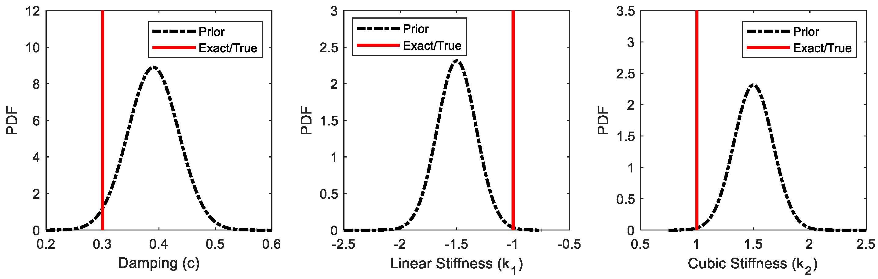
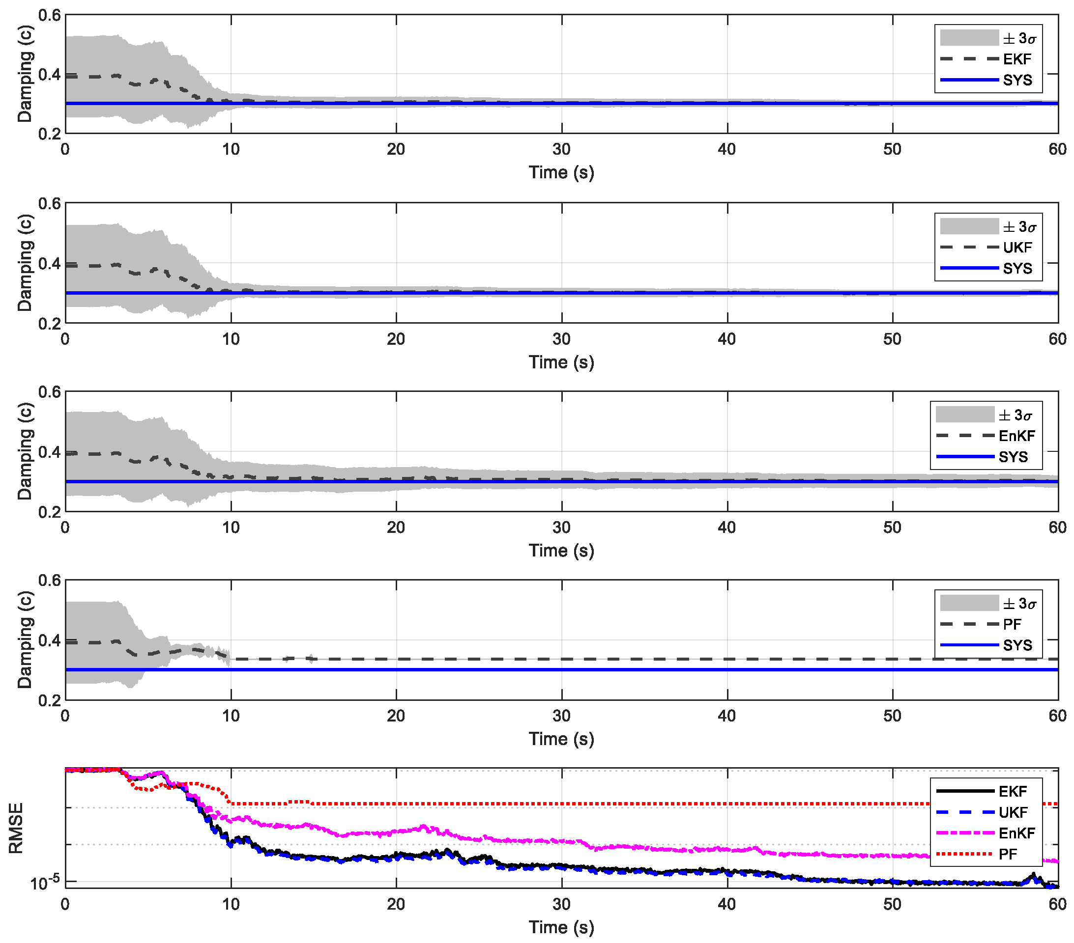
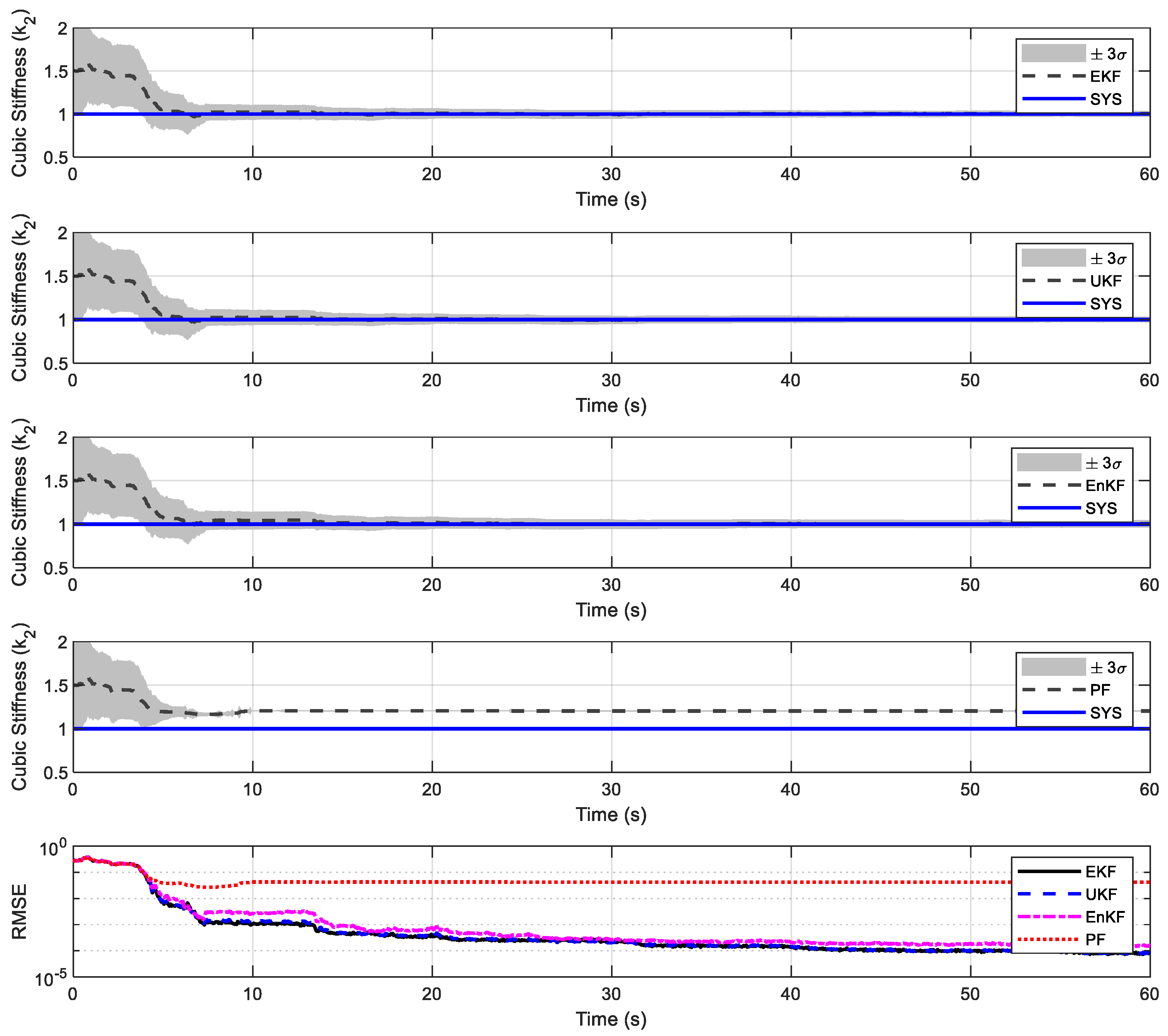
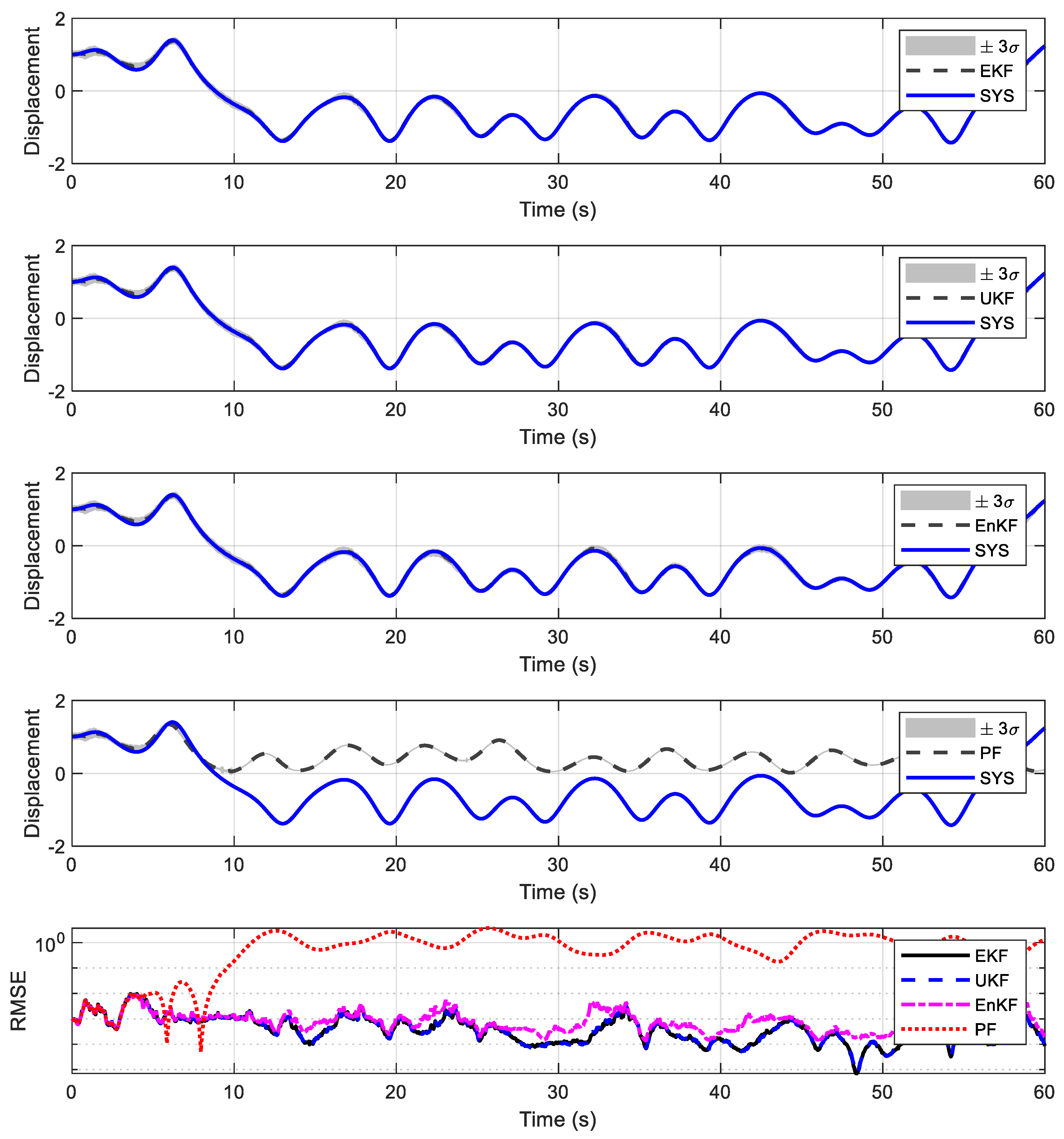
4.1. Duffing Oscillator

The Duffing oscillator dynamics are modeled by the following:

$$\mathrm{m}\ddot{q}\left(t\right)+\mathrm{c}\dot{q}\left(t\right)+{\mathrm{k}}_{1}q\left(t\right)+{\mathrm{k}}_2{q}^3\left(t\right)=u\left(t\right)$$

(22)

where $\mathrm{m}$ is the oscillator mass, $\mathrm{c}$ is the damping coefficient, and ${\mathrm{k}}_1$ and ${\mathrm{k}}_2$ are, respectively, the linear and cubic stiffness coefficients. The Duffing oscillator shows a wide variety of nonlinear response features, and it is applied to model the behavior of many mechanical, structural, and electrical systems, such as the restoring characteristics of deformable solids, buckling of slender members, nonlinearity in circuits, superconductors, and the chaotic behavior of dynamical systems in different domains, among others [47].

The exact/true system parameters used to generate the data are (in consistent SI units) $\mathrm{m}=1 \mathrm{k}\mathrm{g}$, $\mathrm{c}=0.3 \mathrm{N}\mathrm{s}/\mathrm{m}$, ${\mathrm{k}}_1=-1 \mathrm{N}/\mathrm{m}$ and ${\mathrm{k}}_2=1 \mathrm{N}/{\mathrm{m}}^3$. For these parameter values under free vibration, the unforced system has three fixed points, namely, an unstable fixed point at 0 and two stable fixed points at 1 and −1. We consider the case where the system is driven by the deterministic harmonic input $u\left(t\right)=0.3cos\left(1.25t\right)\mathrm{N}$; under this condition, the system exhibits two period-two subharmonic oscillations [30]. The initial conditions are selected as $q\left(0\right)=1$ and $\dot{q}\left(0\right)=0$. To solve the forward problem and to perform the estimation, the system is discretized using the fourth-order Runge–Kutta method with time step $∆t=0.005 \mathrm{s}$.

The objective is to estimate the parameters vector $\theta$ = {$\mathrm{c}$ ${\mathrm{k}}_1$ ${\mathrm{k}}_2$} assumed to be uncertain/unknown. To perform Bayesian system identification, an initial prior distribution for the parameters needs to be specified. Figure 1 shows the prior distributions adopted and the system’s exact/true parameters. Significant uncertainty about the true values of the parameters has been assumed, with the true parameters falling on the tails of the prior distributions and initial errors between 30% and 50%; the algorithms were initialized with different sets of initial estimates, and no significant variation in the results was observed. The measurement data used for estimation consists of a noise-contaminated displacement response, with the noise modeled as Gaussian white noise with a 10% noise-to-signal root-mean-square (RMS). The noise model is consistent with models for this type of sensor [48]. It was observed that the performance of the filters did not change significantly with RMS values of up to 20%.

The UKF was implemented using the scaled unscented transform algorithm with the scale parameter selected as $\alpha ={10}^{-3}$ based on previous filter performance assessments [45]. The sample size for the EnKF was selected as $N=2000$; the sample size was selected based on a convergence analysis where the sample size was increased until no significant variation in the estimates was observed. The PF was applied using the sequential importance sampling (SIS) algorithm with resampling, also known as the bootstrap filter [46], combined with the parallelized implementation proposed in Ref. [20] to reduce and delay sample degeneracy. The weight coefficient of the variation threshold for resampling was selected as 3, with 20 parallel particle filters, each running with 4000 particles. For the PF, increasing the sample size reduces sample degeneracy and improves the estimation; however, there are computational limitations to the sample size due to limited computer memory and the required computational time; the sample size of 80,000 total particles selected is close to the maximum that a standard desktop computer memory allows. The use of high-performance computing systems is needed to further increase the sample size at the expense of a high computational effort. For most practical applications, the availability of such high-performance computing systems is limited.

Figure 2, Figure 3 and Figure 4 show the estimation results for the oscillator damping, linear stiffness, and cubic stiffness parameters, respectively; the figures show the mean estimate and the uncertainty bounds defined as ±3 standard deviations, with ‘SYS’ indicating the exact/true system response. The root-mean-square error (RMSE) is used as a measure of the estimation accuracy of the filters; the RMSE of the estimate $\widehat{\phi }$ of the true/exact parameter $\phi$ is defined as $\mathrm{R}\mathrm{M}\mathrm{S}\mathrm{E}=\sqrt{\mathbb{E}\left[{\left(\widehat{\phi }-\phi \right)}^2\right]}$ where $\mathbb{E}\left[·\right]$ is the expectation operator, and the estimate $\widehat{\phi }$ is a random variable. The RMSE allows us to quantify the estimation accuracy by accounting for both estimation bias and uncertainty, and, for this reason, it is widely adopted as an estimation accuracy metric; if two estimators are unbiased, then the estimator with larger uncertainty would result in a larger RMSE. Figure 2, Figure 3 and Figure 4 show that the EKF, UKF, and EnKF successfully estimate all the oscillator parameters, with the PF not showing convergence to the exact parameters’ values. It is interesting to note that the EKF provided good estimation results for this example, in agreement with the results reported in Ref. [30]. This is attributed to the time step $∆t=0.005$ used for the simulations, which is considered small for the characteristic time scale of the system’s dynamic behavior, resulting in improved accuracy of the linearization employed by the EKF.

Based on the particle’s coefficient of variation, the PF showed particle degeneracy at approximately $t=5 \mathrm{s}$. This is confirmed by Figure 2, Figure 3 and Figure 4, and particularly the RMSE, which show that all the filters provide comparable estimates, uncertainty, and accuracy up to $t=5 \mathrm{s}$; after this time, all the particles of the PF collapsed into a single particle, and the sample was no longer able to properly approximate the parameters posterior distribution. The PF RMSE is seen to remain large when compared to the RMSE of the other filters. It is worth pointing out that the main factor defining the onset of particle degeneracy is the number of analysis time steps. In the case of the present example, degeneracy started after 1000 steps. A strategy to attempt to delay the onset of particle degeneracy is to downsample the measurements by not updating the posterior distribution at every time step, that is, not using all the available measurements; this approach was successfully employed in Ref. [30] to improve the accuracy of the PF. This strategy is adopted at the expense of significantly decreasing the sampling frequency, which is not ideal in applications since it is desirable to fully exploit and extract the information available on the measurements. Moreover, downsampling the measurements has an impact on the accuracy and significantly increases the estimate’s uncertainty. Another strategy to delay particle degeneracy is to include a fictitious process noise that inflates the particles’ variance. Although this strategy, in general, improves the estimation accuracy of filtering methods by increasing the parameter uncertainty, it does not resolve the particle degeneracy issue nor significantly delay the particle’s collapse. Including a fictitious noise is considered a heuristic, and there are no rigorous methods to define the variance of the noise or how much fictitious uncertainty should be introduced to the problem.

From a theoretical point of view, the only approach to effectively delay particle degeneracy is to modify the proposal distribution using improved estimates obtained, for example, using a Gaussian mixture model (Gaussian mixture sigma-point particle filter), a model linearization (Extended particle filter), or the unscented transform (Unscented particle filter). Although the more refined versions of the particle filter delay the onset of particle degeneracy, the issue still persists, with the particles eventually concentrating on small regions of the probability space, albeit a few time steps after the standard PF [24].

Figure 5 and Figure 6 show the estimates of the oscillator displacement and velocity, respectively. All the filters show a state estimation accuracy comparable to the parameter estimation, with the PF showing degradation due to particle degeneracy. Similarly to the parameter estimation results, the PF dynamic response estimates and uncertainty are in agreement with the other filters up to $t=5 \mathrm{s}$, the approximate time instant at which the particle sample collapses to a single particle. In addition to the accuracy of the filters, the computational effort and efficiency are also of importance for implementation in practice. The computational time (in seconds) required by the filters was, for the EKF, 500 s, for the UKF, 2 s, for the EnKF, 90 s, and, for the PF, 5370 s. The results show that the UKF is the most efficient estimation algorithm with good accuracy at an affordable computational cost. Most of the computational time required for the EKF is used in the computation of the gradient required to linearize the model. The EnKF and PF are computationally intensive and not suitable for online or real-time applications due to the effort required to project/update the large set of sample points/particles employed by the algorithms. The RMSE of the estimates providing a measure of the accuracy of the four filters is summarized in

Table 1. RMSE summary for the Duffing oscillator example.

	$\mathbf{c} \mathbf{(}\mathbf{N}\mathbf{s}\mathbf{/}\mathbf{m}\mathbf{)}$	${\mathbf{k}}_{\mathbf{1}} \mathbf{(}\mathbf{N}\mathbf{/}\mathbf{m}\mathbf{)}$	${\mathbf{k}}_{\mathbf{2}} \mathbf{(}\mathbf{N}\mathbf{/}{\mathbf{m}}^{\mathbf{3}}\mathbf{)}$
EKF	$7.4\times {10}^{-6}$	$6.7\times {10}^{-5}$	$7.9\times {10}^{-5}$
UKF	$7.4\times {10}^{-6}$	$6.7\times {10}^{-5}$	$7.9\times {10}^{-5}$
EnKF	$4.8\times {10}^{-5}$	$1.5\times {10}^{-4}$	$1.5\times {10}^{-4}$
PF	$0.0012$	$0.03$	$0.04$

.

4.2. Bouc–Wen Hysteretic Oscillator

In this section, we consider a nonlinear hysteretic oscillator of the Bouc–Wen type [49]. The development of response and parameter estimation methods in the context of hysteretic models has received notable attention in recent decades due to their application in the modeling of material nonlinearity and inelastic behavior in structural mechanics, including low-cycle damage due to severe loading and high-cycle accumulated fatigue [50,51,52,53,54,55]. The dynamic behavior of an oscillator with a Bouc–Wen model for hysteresis is governed by the following equation:

$$\mathrm{m}\ddot{q}\left(t\right)+\mathrm{c}\dot{q}\left(t\right)+{\mathrm{D}}_{\mathrm{y}}\mathrm{k}z\left(t\right)=u\left(t\right)$$

(23)

where $\mathrm{k}$ is the initial stiffness and ${\mathrm{D}}_{\mathrm{y}}$ is the yielding displacement. The normalized hysteretic force variable $z$ is governed by the following:

$$\dot{z}\left(t\right)={\displaystyle \frac{1}{{\mathrm{D}}_{\mathrm{y}}}}\left[\dot{q}\left(t\right)-\beta \left|\dot{q}\left(t\right)\right|{\left|z\left(t\right)\right|}^{\nu -1}z\left(t\right)-\gamma \dot{q}\left(t\right){\left|z\left(t\right)\right|}^{\nu } \right]$$

(24)

where $\beta$, $\gamma ,$ and $\nu$ define the shape and geometry of the hysteresis loops including the transition between elastic and plastic behavior regimes. The parameters $\beta$ and $\gamma$ are not unique when treated independently, and the constraint $\beta +\gamma =1$ is used to enforce uniqueness; this implies that only one of the parameters needs to be estimated [49]. Without loss of generality, the parameter $\beta$ is estimated, and the parameter $\gamma$ is readily computed from the constraint equation.

The true/exact system parameters used to generate the data are as follows (in consistent SI units): $\mathrm{m}=1 \mathrm{k}\mathrm{g}$, $\mathrm{k}=9 \mathrm{N}/\mathrm{m}$, ${\mathrm{D}}_{\mathrm{y}}=0.3 \mathrm{m}$, $\beta =0.2$, $\nu =2$, and a 5% damping ratio. The oscillator is excited by a base acceleration, ${\ddot{u}}_g$, in which case the forcing input is $u=-m{\ddot{u}}_g$. To solve the forward problem and to perform the estimation, the system is time discretized using the fourth-order Runge–Kutta method with time step $∆t=0.005 \mathrm{s}$. The objective is to estimate the nonlinear parameters vector $\theta$ = {${\beta \mathrm{D}}_{\mathrm{y}} \nu$}, which is assumed to be uncertain/unknown. The measurement data used for estimation consists of noise-contaminated absolute acceleration response with a 10% noise-to-signal RMS. The nonlinear Bayesian filters are implemented using the filter parameters of the previous section. The prior distributions adopted for the parameters are depicted in Figure 7, which shows that initial errors between 60 and 100% are assumed for all the parameters. The figure also shows that significant uncertainty about the true values of the parameters is accounted for in the analysis. The level of uncertainty in the prior distributions adopted are in agreement with the expected level of prior knowledge about structural nonlinear parameters where nonlinear parameters show significant uncertainty and variability.

Figure 8, Figure 9 and Figure 10 show the estimation results for the nonlinear hysteresis geometry parameters; the figures show the mean estimate and the uncertainty bounds defined as ±3 standard deviations. The figures show that the EKF, UKF, and EnKF are able to successfully estimate the oscillator nonlinear parameters, while the PF shows convergence difficulties. Similarly to the previous example, based on the particle’s coefficient of variation, the particle degeneracy was detected at $t=2 \mathrm{s}$, which can be confirmed from the estimated time histories by noting the rapid collapse of the uncertainty bounds at this time when compared to the other filters. The reduction in the PF uncertainty bounds at $t=2 \mathrm{s}$ is not related to the updating of the posterior distribution as more data becomes available, and instead is a limitation of the algorithm due to the importance distribution adopted that results in a rapid collapse of the particles; the uncertainty reduction is a fictitious artifact due to the collapse and not representative of the actual distribution uncertainty, which can be verified by comparing the uncertainty bounds provided by the other filters. The RMSE of the estimates providing a measure of the accuracy of the four filters is summarized in

Table 2. RMSE summary for the Bouc–Wen oscillator example.

	$\mathit{\beta }$	$\mathit{\nu }$	${\mathbf{D}}_{\mathbf{y}} \mathbf{\left(}\mathbf{m}\mathrm{\right)}$
EKF	$2.6\times {10}^{-5}$	$1.1\times {10}^{-4}$	$7.2\times {10}^{-5}$
UKF	$1.9\times {10}^{-5}$	$1.3\times {10}^{-2}$	$1.2\times {10}^{-3}$
EnKF	$2.0\times {10}^{-5}$	$1.2\times {10}^{-2}$	$1.2\times {10}^{-3}$
PF	$0.25$	$3.12$	$0.15$

.

Figure 11 shows the displacement estimates provided by all the filters, while Figure 12 shows the force–displacement histories, which depict the hysteretic behavior. The UKF shows the best hysteretic response tracking capabilities, followed by the EnKF and EKF.

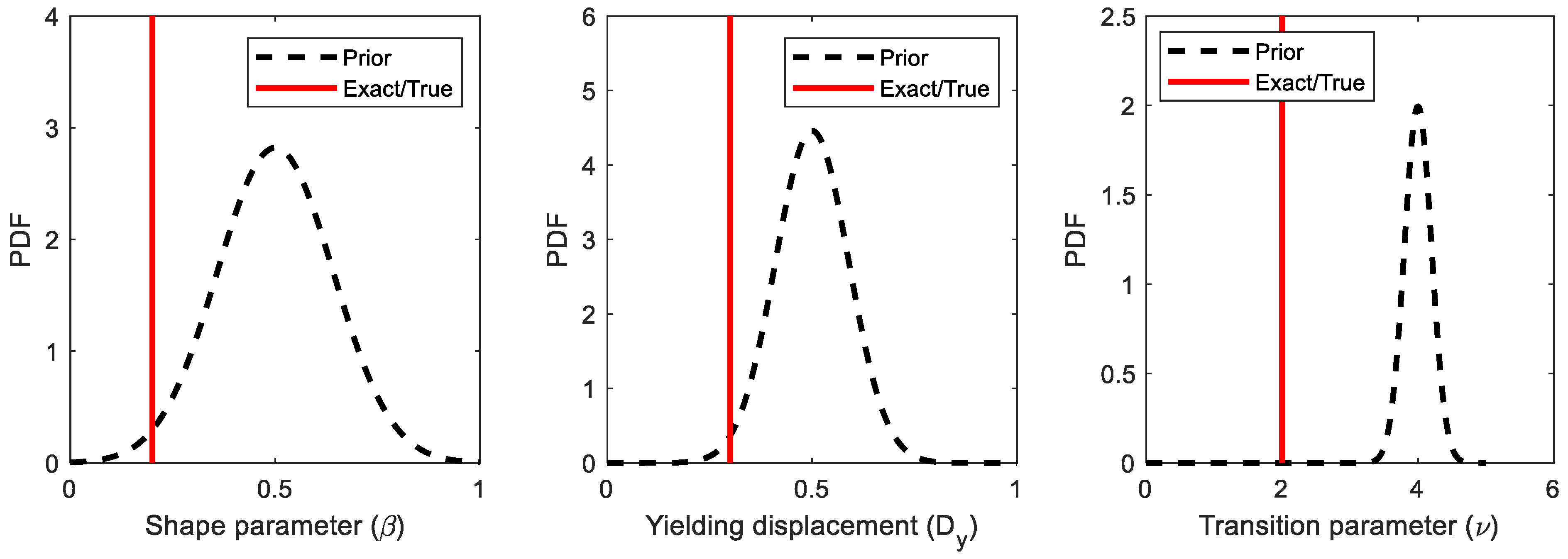
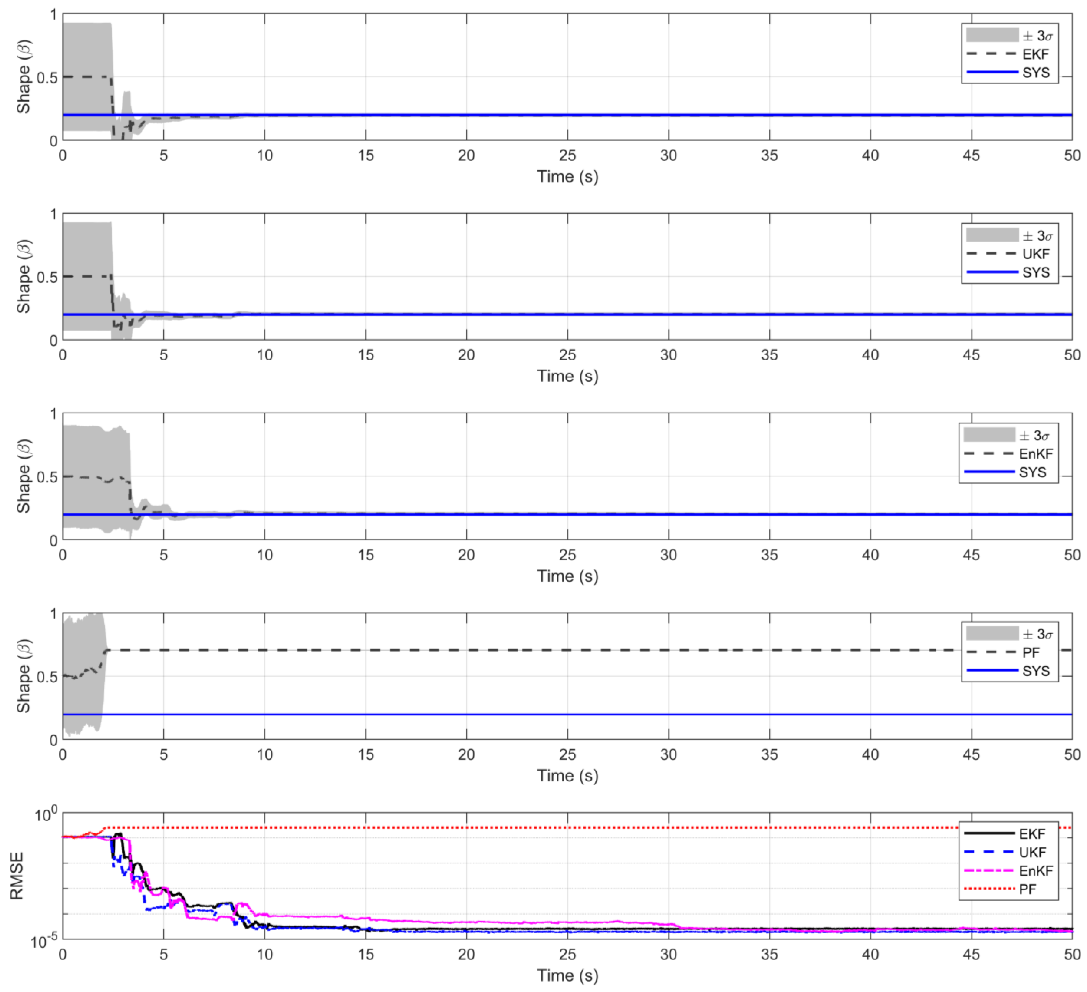
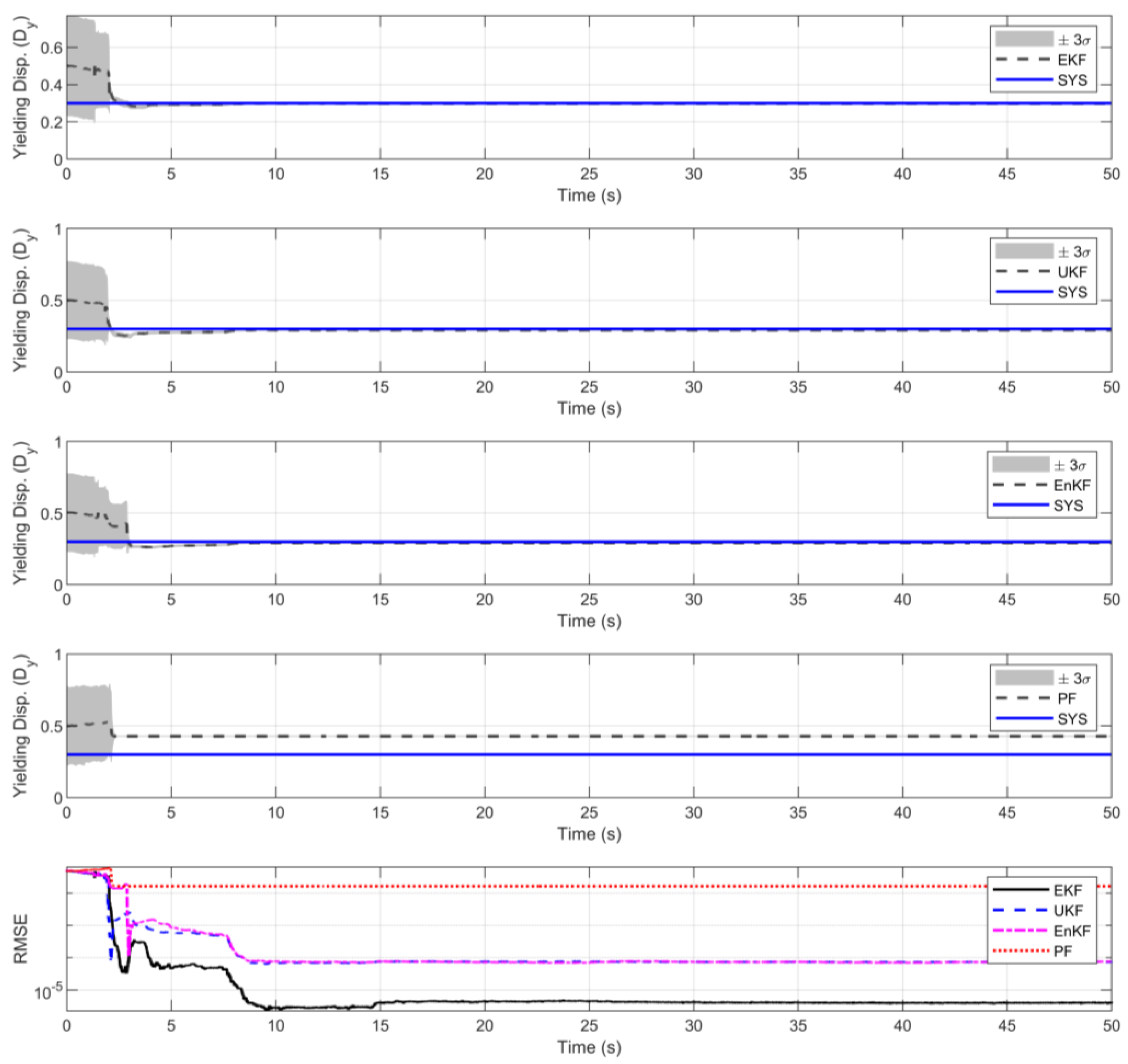
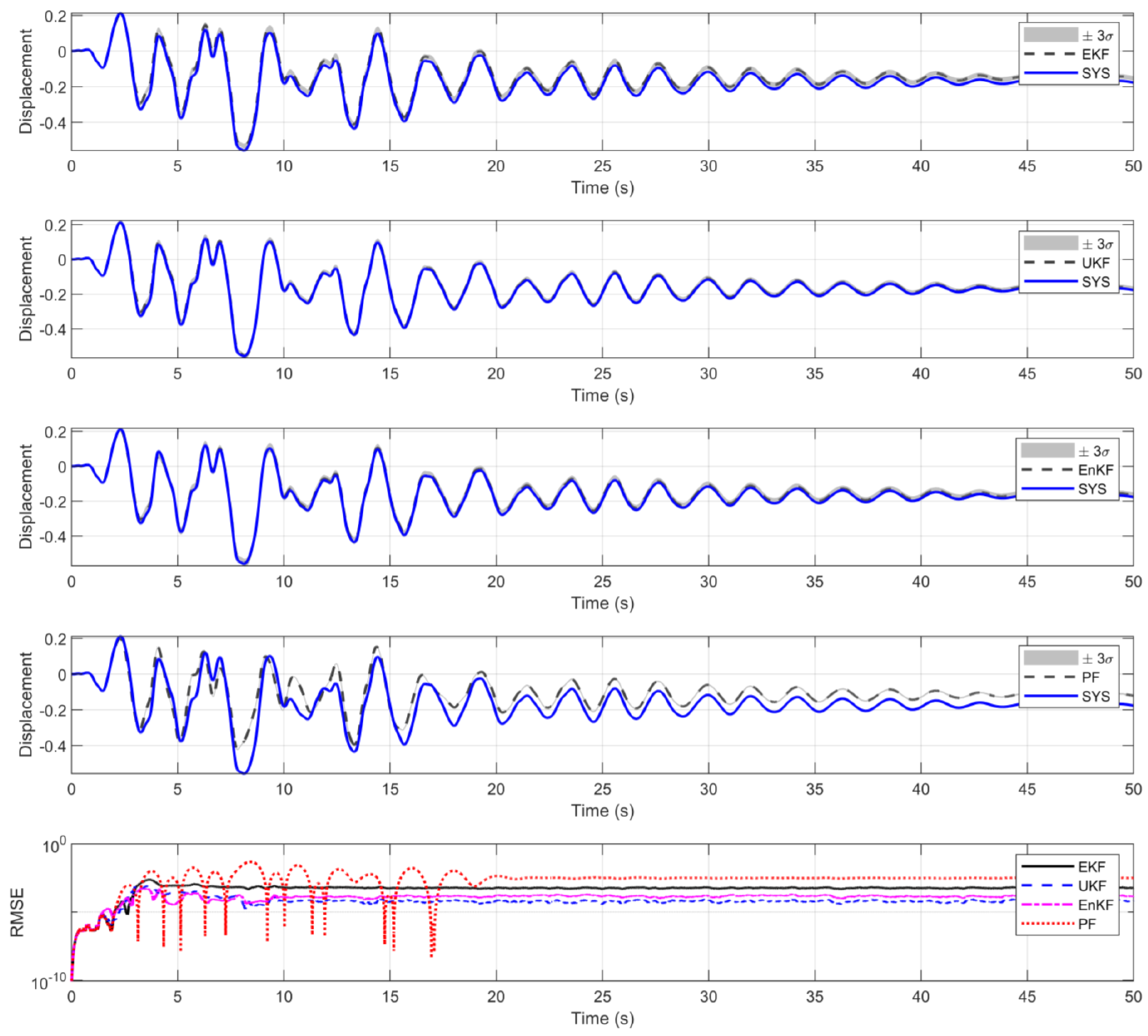
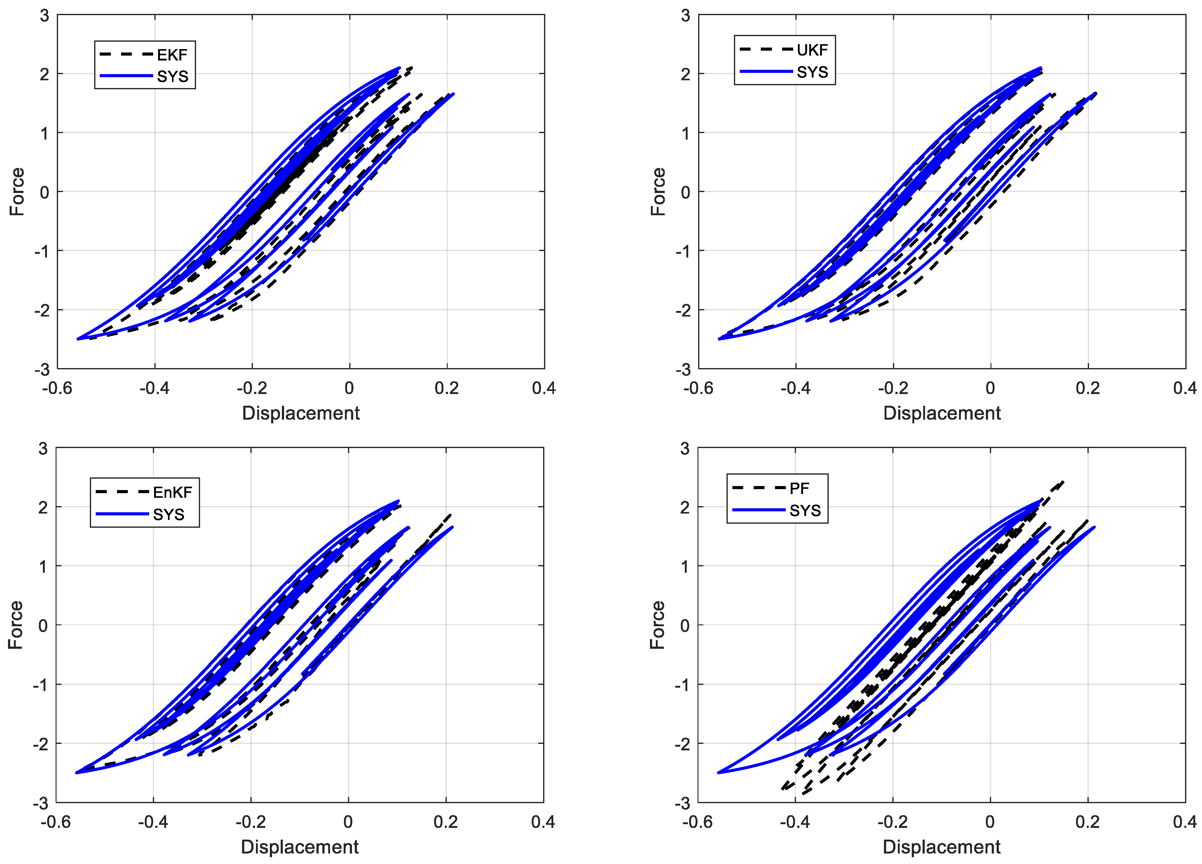
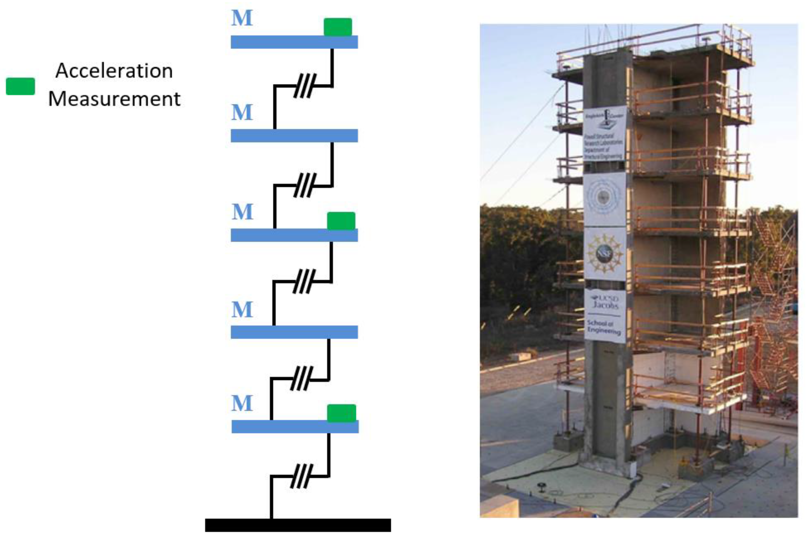
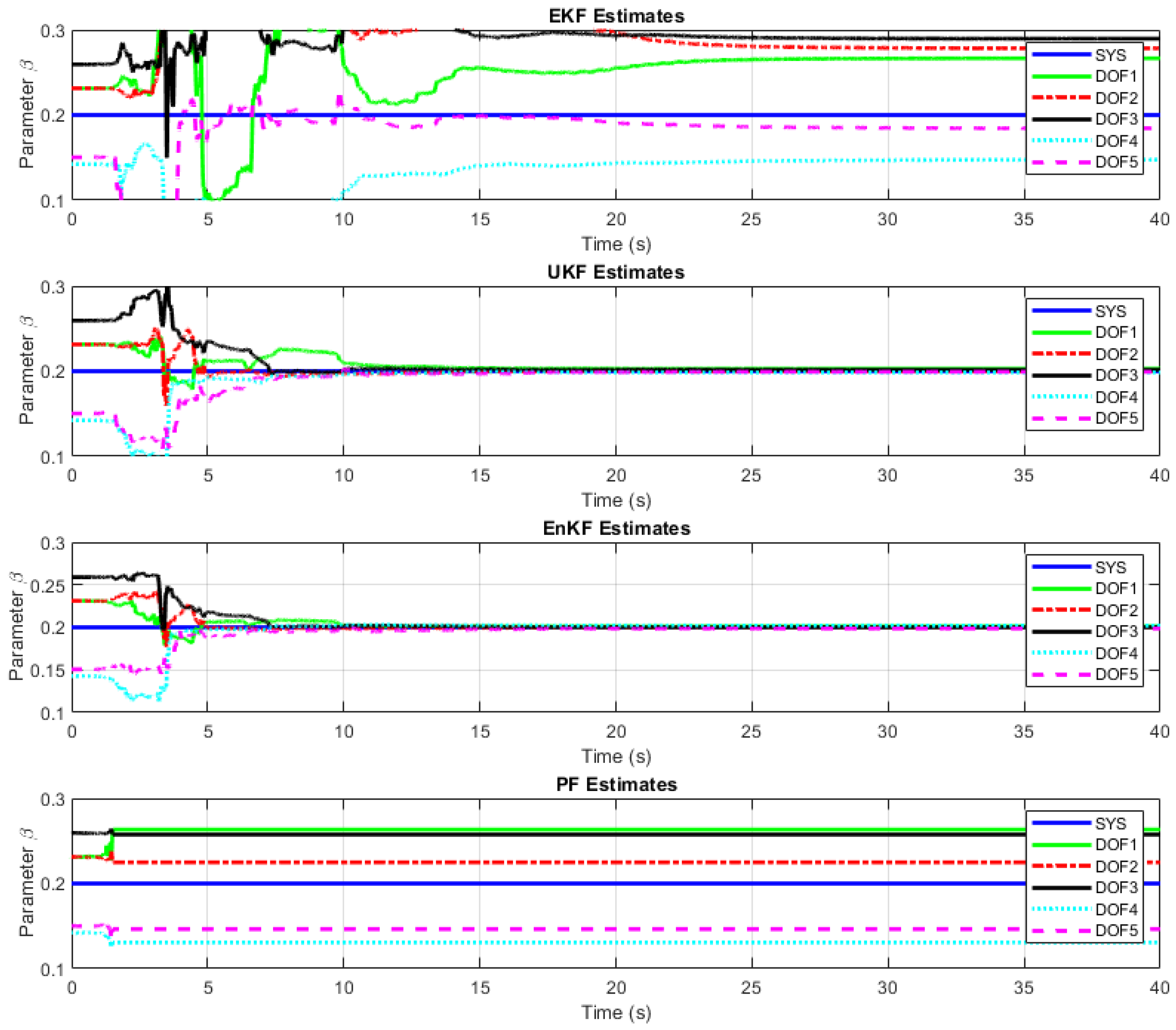
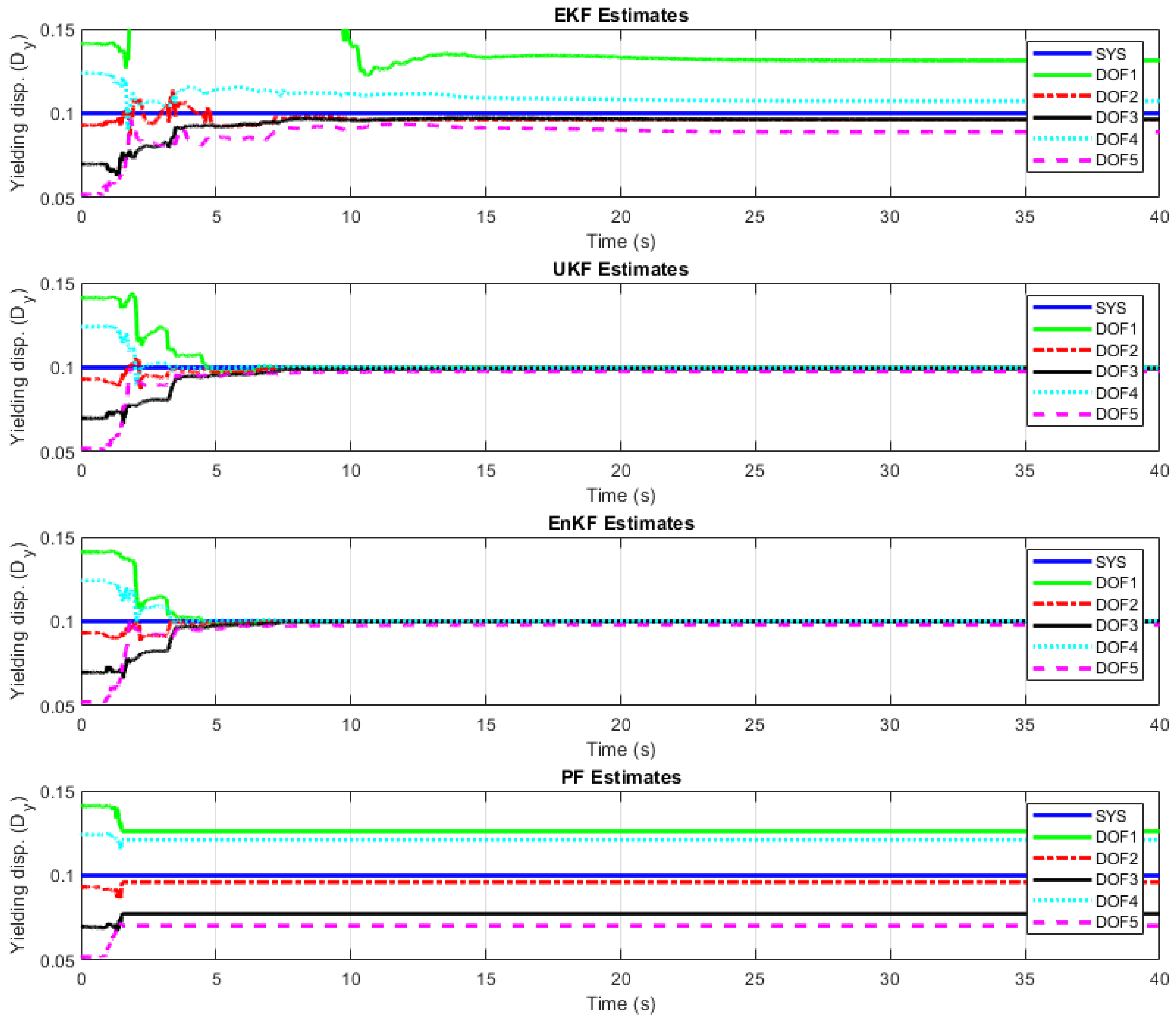
4.3. Bouc–Wen Hysteretic Chain System

In this section, we study the scalability of the methods for a system with an increased number of parameters and limited response measurements. For this purpose, we consider a five-degrees-of-freedom chain-type system, where each spring of the chain is governed by the hysteretic Bouc–Wen model discussed in the previous section. The mass and restoring force characteristics of the system are shown in the left panel of Figure 13. Damping is modeled as modal damping with a 5% damping ratio for all modes, computed based on the initial linear properties of the system.

The true/exact system parameters are selected as follows (in consistent SI units). The mass and initial linear stiffness (for all springs) are $\mathrm{M}=4.3\times {10}^4$ and $\mathrm{k}=2\times {10}^7.$ The hysteretic parameters for all the springs are selected as ${\mathrm{D}}_{\mathrm{y}}=0.10$, $\beta =0.20$, and $\nu =2$. The parameters are selected to be consistent with the parameters of the reinforced concrete structure tested on a shake table shown in Figure 13 [56,57]. The system is excited by a base acceleration consisting of a record of the 1994 Northridge earthquake. The objective is to estimate the parameters vector $\theta$ = {$\beta$ ${\mathrm{D}}_{\mathrm{y}}$ $\nu$} for each of the five springs of the model. The measurement data used for estimation consist of the noise-contaminated absolute acceleration response of degrees-of-freedom 1, 3, and 5, with a 10% noise-to-signal RMS (see Figure 13). Note that, in this study, we focus on the parameters of the system; for a related study focused on seismic response reconstruction, the interested reader can consult Ref. [57].

The nonlinear Bayesian filters are implemented using the filter parameters discussed in the previous section. The parameters prior distributions are selected with random initial errors between 25% and 75% for all the parameters and a coefficient of variation of 5%. Note that the dimension of the augmented state for this example is $x\in {\mathbb{R}}^{30}$, with three dynamic response variables and three parameters for each degree of freedom. The relationship between the dimension of the state and the number, type, and location of measured outputs is the main factor determining the accuracy and capability of the estimators to successfully infer the parameters (identifiability), with scalability and identifiability limitations arising as the dimension of the augmented state increases, an issue known as the curse of dimensionality. Moreover, the use of absolute acceleration measurements, usually used in practice due to the affordability of accelerometer sensors, presents an increased challenge in the estimation of nonlinear parameters with reduced identifiability with respect to other types of measurements, such as displacements [58].

Figure 14, Figure 15 and Figure 16 show the estimation results for the hysteresis shape parameter, the yielding displacement, and the linear–inelastic transition parameter, respectively; the figures show the mean estimates for the springs of each degree of freedom. The figures show that only the UKF and EnKF are able to successfully estimate the nonlinear parameters of the system. The PF shows the same particle degeneracy issue of previous examples, although the issue is exacerbated by the dimension of the augmented state. It is interesting to note the degradation of the estimation accuracy of the EKF with respect to the oscillator counterpart. As shown in Section 4.2, the EKF was able to estimate the single-degree-of-freedom hysteretic oscillator parameters, while, in this section, the EKF estimates are not accurate under an increased dimension of the augmented state and the use of limited acceleration measurements. On the other hand, the UKF and EnKF were able to maintain a comparable level of accuracy.

Finally, it is interesting to note that the computational time required by the filters for this example were EKF—4 h, UKF—19 min, EnKF—5 h, and PF—50 h. Thus, the UKF is the most efficient estimation algorithm with an accuracy comparable to the EnKF at a significantly reduced computational cost.

5. Conclusions

This paper examined the performance of nonlinear Bayesian filtering when applied to the identification of the parameters of structural and mechanical systems. This study employed metrics to assess the accuracy and limitations of the four most well-established nonlinear filtering methods: the extended Kalman filter (EKF), the unscented Kalman filter (UKF), the ensemble Kalman filter (EnKF), and the particle filter (PF). The filtering methods were applied to estimate the parameters and the response of three benchmark dynamical systems used in structural mechanics, namely, a Duffing oscillator, a hysteretic oscillator, and a hysteretic chain-type system.

For the single-degree-of-freedom oscillators, the EKF and UKF converged to the true system parameters with a comparable estimation accuracy, with the EKF showing a higher computational cost. In the case of multiple degrees-of-freedom systems, the EKF was not able to scale appropriately to large parameter spaces, while the UKF preserved the estimation accuracy observed for the oscillators. In the case of the EnKF, the algorithm provided estimates of the same order of accuracy as the UKF, albeit at a significantly higher computational cost that was on the order of several hours. The PF was not able to converge to the true parameters for any of the systems studied, with the particles showing severe degeneracy, collapsing to a reduced subset of the parameter space after a few implementation steps. Based on the performance, accuracy, and computational efficiency of the methods under different operating conditions, it is concluded that the UKF is the most effective filtering-based system identification method for the type of systems considered herein, showing a stable estimation accuracy for parameter spaces considered of high dimension in applications.

References

1. Grigoriu, M. Stochastic Systems: Uncertainty Quantification and Propagation; Springer Science & Business Media: Berlin/Heidelberg, Germany, 2012. [Google Scholar]
2. Ljung, L. System Identification. In Signal Analysis and Prediction; Procházka, A., Uhlíř, J., Rayner, P.W.J., Kingsbury, N.G., Eds.; Birkhäuser Verlag: Basel, Switzerland, 1998. [Google Scholar]
3. Maia, N.M.M.; Montalvão Silva e Silva, J.M. Theoretical and Experimental Modal Analysis; Wiley: Hoboken, NJ, USA, 1997. [Google Scholar]
4. Kerschen, G.; Worden, K.; Vakakis, A.F.; Golinval, J.-C. Past, present and future of nonlinear system identification in structural dynamics. Mech. Syst. Signal Process. 2005, 20, 505–592. [Google Scholar] [CrossRef]
5. Moaveni, B.; He, X.; Conte, J.P.; Restrepo, J.I. Damage identification study of a seven-story full-scale building slice tested on the UCSD-NEES shake table. Struct. Saf. 2010, 32, 347–356. [Google Scholar] [CrossRef]
6. Ortiz, G.A.; Alvarez, D.A.; Bedoya-Ruíz, D. Identification of Bouc–Wen type models using multi-objective optimization algorithms. Comput. Struct. 2013, 114–115, 121–132. [Google Scholar] [CrossRef]
7. Beck, J.L. Bayesian system identification based on probability logic. Struct. Control Health Monit. 2010, 17, 825–847. [Google Scholar] [CrossRef]
8. Yuen, K.V.; Mu, H.Q. Real-time system identification: An algorithm for simultaneous model class selection and parametric identification. Comput.-Aided Civ. Infrastruct. Eng. 2015, 30, 785–801. [Google Scholar] [CrossRef]
9. Behmanesh, I.; Moaveni, B.; Lombaert, G.; Papadimitriou, C. Hierarchical Bayesian model updating for structural identification. Mech. Syst. Signal Process. 2015, 64, 360–376. [Google Scholar] [CrossRef]
10. Yuen, K.V.; Kuok, S.C.; Dong, L. Self-calibrating Bayesian real-time system identification. Comput.-Aided Civ. Infrastruct. Eng. 2019, 34, 806–821. [Google Scholar] [CrossRef]
11. Jazwinski, A.H. Stochastic Processes and Filtering Theory; Courier Corporation: Chelmsford, MA, USA, 2007. [Google Scholar]
12. Kalman, R.E. A New Approach to Linear Filtering and Prediction Problems. J. Basic Eng. 1960, 82, 35–45. [Google Scholar] [CrossRef]
13. Simon, D. Optimal State Estimation: Kalman, H Infinity, and Nonlinear Approaches; John Wiley and Sons: Hoboken, NJ, USA, 2006. [Google Scholar]
14. Julier, S.; Uhlmann, J. A new extension of the Kalman filter to nonlinear systems. In The Robotic Research Group Report; The University of Oxford: Oxford, UK, 1997. [Google Scholar]
15. Evensen, G. The Ensemble Kalman Filter: Theoretical formulation and practical implementation. Ocean. Dyn. 2003, 53, 343–367. [Google Scholar] [CrossRef]
16. Doucet, A.; Godsill, S.; Andrieu, C. On sequential Monte Carlo sampling methods for Bayesian filtering. Stat. Comput. 2000, 10, 197–208. [Google Scholar] [CrossRef]
17. Corigliano, A.; Mariani, S. Parameter identification in explicit structural dynamics: Performance of the extended Kalman filter. Comput. Methods Appl. Mech. Eng. 2004, 193, 3807–3835. [Google Scholar] [CrossRef]
18. Lin, J.W.; Betti, R. On-line identification and damage detection in non-linear structural systems using a variable forgetting factor approach. Earthq. Eng. Struct. Dyn. 2004, 33, 419–444. [Google Scholar] [CrossRef]
19. Ghanem, R.; Ferro, G. Health monitoring for strongly non-linear systems using the Ensemble Kalman filter. Struct. Control Health Monit. 2005, 13, 245–259. [Google Scholar] [CrossRef]
20. Ching, J.; Beck, J.; Porter, K.; Shaikhutdinov, R. Bayesian state estimation method for nonlinear systems and its application to recorded seismic response. ASCE J. Eng. Mech. 2006, 132, 396–410. [Google Scholar] [CrossRef]
21. Yang, J.N.; Lin, S.; Huang, H.; Zhou, L. An adaptive extended Kalman filter for structural damage identification. Struct. Control Health Monit. 2006, 13, 849–867. [Google Scholar] [CrossRef]
22. Namdeo, V.; Manohar, C. Nonlinear structural dynamical system identification using adaptive particle filters. J. Sound Vib. 2007, 306, 524–563. [Google Scholar] [CrossRef]
23. Wu, M.; Smyth, A.W. Application of the unscented Kalman filter for real-time nonlinear structural system identification. Struct. Control Health Monit. 2007, 14, 971–990. [Google Scholar] [CrossRef]
24. Chatzi, E.N.; Smyth, A.W. The unscented Kalman filter and particle filter methods for nonlinear structural system identification with non-collocated heterogeneous sensing. Struct. Control Health Monit. 2009, 16, 99–123. [Google Scholar] [CrossRef]
25. Lourens, E.; Papadimitriou, C.; Gillijns, S.; Reynders, E.; De Roeck, G.; Lombaert, G. Joint input-response estimation for structural systems based on reduced-order models and vibration data from a limited number of sensors. Mech. Syst. Signal Process. 2012, 29, 310–327. [Google Scholar] [CrossRef]
26. Xu, B.; He, J.; Rovekamp, R.; Dyke, S.J. Structural parameters and dynamic loading identification from incomplete measurements: Approach and validation. Mech. Syst. Signal Process. 2012, 28, 244–257. [Google Scholar] [CrossRef]
27. Chatzis, M.; Chatzi, E.; Smyth, A. An experimental validation of time domain system identification methods with fusion of heterogeneous data. Earthq. Eng. Struct. Dyn. 2014, 44, 523–547. [Google Scholar] [CrossRef]
28. Sun, H.; Betti, R. Simultaneous identification of structural parameters and dynamic input with incomplete output-only measurements. Struct. Control Health Monit. 2014, 21, 868–889. [Google Scholar] [CrossRef]
29. Azam, S.E.; Chatzi, E.; Papadimitriou, C. A dual Kalman filter approach for state estimation via output-only acceleration measurements. Mech. Syst. Signal Process. 2015, 60, 866–886. [Google Scholar] [CrossRef]
30. Khalil, M.; Sarkar, A.; Adhikari, S.; Poirel, D. The estimation of time-invariant parameters of noisy nonlinear oscillatory systems. J. Sound Vib. 2015, 344, 81–100. [Google Scholar] [CrossRef]
31. Liu, L.; Su, Y.; Zhu, J.; Lei, Y. Data fusion based EKF-UI for real-time simultaneous identification of structural systems and unknown external inputs. Measurement 2016, 88, 456–467. [Google Scholar] [CrossRef]
32. Maes, K.; Smyth, A.; De Roeck, G.; Lombaert, G. Joint input-state estimation in structural dynamics. Mech. Syst. Signal Process. 2016, 70–71, 445–466. [Google Scholar] [CrossRef]
33. Yan, G.; Sun, H.; Büyüköztürk, O. Impact load identification for composite structures using Bayesian regularization and unscented Kalman filter. Struct. Control Health Monit. 2016, 24, e1910. [Google Scholar] [CrossRef]
34. Erazo, K.; Nagarajaiah, S. An offline approach for output-only Bayesian identification of stochastic nonlinear systems using unscented Kalman filtering. J. Sound Vib. 2017, 397, 222–240. [Google Scholar] [CrossRef]
35. Erazo, K.; Nagarajaiah, S. Bayesian structural identification of a hysteretic negative stiffness earthquake protection system using unscented Kalman filtering. Struct. Control Health Monit. 2018, 25, e2203. [Google Scholar] [CrossRef]
36. Erazo, K.; Sen, D.; Nagarajaiah, S.; Sun, L. Vibration-based structural health monitoring under changing environmental conditions using Kalman filtering. Mech. Syst. Signal Process. 2018, 117, 1–15. [Google Scholar] [CrossRef]
37. Lei, Y.; Xia, D.; Erazo, K.; Nagarajaiah, S. A novel unscented Kalman filter for recursive state-input-system identification of nonlinear systems. Mech. Syst. Signal Process. 2019, 127, 120–135. [Google Scholar] [CrossRef]
38. Kammouh, O.; Gardoni, P.; Cimellaro, G.P. Probabilistic framework to evaluate the resilience of engineering systems using Bayesian and dynamic Bayesian networks. Reliab. Eng. Syst. Saf. 2020, 198, 106813. [Google Scholar] [CrossRef]
39. Ierimonti, L.; Cavalagli, N.; Venanzi, I.; García-Macías, E.; Ubertini, F. A transfer Bayesian learning methodology for structural health monitoring of monumental structures. Eng. Struct. 2021, 247, 113089. [Google Scholar] [CrossRef]
40. Diaz, M.; Charbonnel, P.; Chamoin, L. A new Kalman filter approach for structural parameter tracking: Application to the monitoring of damaging structures tested on shaking-tables. Mech. Syst. Signal Process. 2022, 182, 109529. [Google Scholar] [CrossRef]
41. Yu, X.; Li, X.; Bai, Y. Evaluating maximum inter-story drift ratios of building structures using time-varying models and Bayesian filters. Soil Dyn. Earthq. Eng. 2022, 162, 107496. [Google Scholar] [CrossRef]
42. Hu, L.; Bao, Y.; Sun, Z.; Meng, X.; Tang, C.; Zhang, D. Outlier Detection Based on Nelder-Mead Simplex Robust Kalman Filtering for Trustworthy Bridge Structural Health Monitoring. Remote Sens. 2023, 15, 2385. [Google Scholar] [CrossRef]
43. Liu, W.; Lai, Z.; Bacsa, K.; Chatzi, E. Neural extended Kalman filters for learning and predicting dynamics of structural systems. Struct. Health Monit. 2023, 23, 1037–1052. [Google Scholar] [CrossRef]
44. Erazo, K.; Di Matteo, A.; Spanos, P. Parameter Estimation of Stochastic Fractional Dynamic Systems Using Nonlinear Bayesian Filtering System Identification Methods. J. Eng. Mech. 2024, 150, 04023117. [Google Scholar] [CrossRef]
45. Julier, S.; Uhlmann, J.; Durrant-Whyte, H.F. A new method for the nonlinear transformation of means and covariances in filters and estimators. IEEE Trans. Autom. Control. 2001, 45, 477–482. [Google Scholar] [CrossRef]
46. Särkkä, S. Bayesian Filtering and Smoothing; Cambridge University Press: Cambridge, UK, 2013. [Google Scholar]
47. Kudryashov, N.A. The generalized Duffing oscillator. Commun. Nonlinear Sci. Numer. Simul. 2021, 93, 105526. [Google Scholar] [CrossRef]
48. Jerath, K.; Brennan, S.; Lagoa, C. Bridging the gap between sensor noise modeling and sensor characterization. Measurement 2018, 116, 350–366. [Google Scholar] [CrossRef]
49. Ikhouane, F.; Rodellar, J. Systems with Hysteresis: Analysis, Identification and Control Using the Bouc-Wen Model; John Wiley & Sons: Hoboken, NJ, USA, 2007. [Google Scholar]
50. Charalampakis, A.E.; Koumousis, V.K. Identification of Bouc–Wen hysteretic systems by a hybrid evolutionary algorithm. J. Sound Vib. 2008, 314, 571–585. [Google Scholar] [CrossRef]
51. Worden, K.; Hensman, J. Parameter estimation and model selection for a class of hysteretic systems using Bayesian inference. Mech. Syst. Signal Process. 2012, 32, 153–169. [Google Scholar] [CrossRef]
52. Omrani, R.; Hudson, R.E.; Taciroglu, E. Parametric identification of nondegrading hysteresis in a laterally and torsionally coupled building using an unscented Kalman filter. J. Eng. Mech. 2013, 139, 452–468. [Google Scholar] [CrossRef]
53. Erazo, K.; Hernandez, E.M. State estimation in nonlinear structural systems. In Nonlinear Dynamics, Volume 2, Proceedings of the 32nd IMAC, A Conference and Exposition on Structural Dynamics, Orlando, FL, USA, 3–6 February 2014; Allen, M., Catbas, F.N., Foss, G., Kerschen, G., Mayes, R., Niezrecki, C., Rixen, D., Atamturktur, H.S., De Clerck, J., Allemang, R.J., et al., Eds.; Springer International Publishing: Berlin/Heidelberg, Germany, 2014; pp. 249–257. [Google Scholar]
54. Erazo, K.; Hernandez, E.M. Uncertainty quantification of state estimation in nonlinear structural systems with application to seismic response in buildings. ASCE-ASME J. Risk Uncertain. Eng. Syst. Part A Civ. Eng. 2016, 2, B5015001. [Google Scholar] [CrossRef]
55. Roohi, M.; Erazo, K.; Rosowsky, D.; Hernandez, E.M. An extended model-based observer for state estimation in nonlinear hysteretic structural systems. Mech. Syst. Signal Process. 2020, 146, 107015. [Google Scholar] [CrossRef]
56. Panagiotou, M.; Restrepo, J.I.; Conte, J.P. Shake-table test of a full-scale 7-story building slice. Phase I: Rectangular wall. J. Struct. Eng. 2011, 137, 691–704. [Google Scholar] [CrossRef]
57. Erazo, K.; Moaveni, B.; Nagarajaiah, S. Bayesian seismic strong-motion response and damage estimation with application to a full-scale seven story shear wall structure. Eng. Struct. 2019, 186, 146–160. [Google Scholar] [CrossRef]
58. Chatzis, M.N.; Chatzi, E.N.; Smyth, A.W. On the observability and identifiability of nonlinear structural and mechanical systems. Struct. Control Health Monit. 2014, 22, 574–593. [Google Scholar] [CrossRef]
Figure 1. Parameters prior distributions for the Duffing oscillator example (in SI units).
Vibration 08 00001 g001
Figure 2. Damping coefficient ( c ) estimates (in Ns/m).
Vibration 08 00001 g002
Figure 3. Linear stiffness coefficient ( k 1 ) estimates (in N/m).
Vibration 08 00001 g003
Figure 4. Cubic stiffness coefficient ( k 2 ) estimates (in N/m3).
Vibration 08 00001 g004
Figure 5. Oscillator displacement estimates (in m).
Vibration 08 00001 g005
Figure 6. Oscillator velocity estimates (in m/s).
Vibration 08 00001 g006
Figure 7. Parameters prior distributions for the hysteretic oscillator example (in SI units).
Vibration 08 00001 g007
Figure 8. Hysteresis shape parameter ( β ) estimates (non-dimensional).
Vibration 08 00001 g008
Figure 9. Yielding displacement parameter ( D y ) estimates (in m).
Vibration 08 00001 g009
Figure 10. Elastic-to-Plastic transition parameter ( ν ) estimates (non-dimensional).
Vibration 08 00001 g010
Figure 11. Oscillator displacement estimates (in m).
Vibration 08 00001 g011
Figure 12. Oscillator force–displacement hysteretic response estimates (in SI units).
Vibration 08 00001 g012
Figure 13. Hysteretic five-degrees-of-freedom chain system.
Vibration 08 00001 g013
Figure 14. Hysteresis parameter ( β ) mean estimates for all degrees of freedom (non-dimensional).
Vibration 08 00001 g014
Figure 15. Yielding displacement parameter ( D y ) mean estimates for all degrees of freedom (in m).
Vibration 08 00001 g015
Figure 16. Elastic-to-Plastic transition parameter ( ν ) mean estimates for all degrees of freedom (non-dimensional).
Vibration 08 00001 g016