Article

Analysis of the Axial Vibration of Non-Uniform and Functionally Graded Rods via an Analytical-Based Numerical Approach

by
Koray Kondakcı
1 and
Safa Bozkurt Coşkun
2,*
1
Institute of Natural and Applied Sciences, Kocaeli University, Kocaeli 41380, Türkiye
2
Department of Civil Engineering, Kocaeli University, Kocaeli 41380, Türkiye
*
Author to whom correspondence should be addressed.
Vibration 2023, 6(4), 876-894; https://doi.org/10.3390/vibration6040052
Submission received: 28 August 2023 / Revised: 7 October 2023 / Accepted: 10 October 2023 / Published: 12 October 2023

Abstract

:
In this study, an analytical-based numerical approach was proposed for the analysis of the free axial vibration of homogeneous and functionally graded rods with varying cross-sectional areas. The proposed approach is based on analytical approximation techniques, such as the Adomian decomposition method, variational iteration method, and homotopy perturbation method. However, the governing equations of the problems solved in this study were variable coefficient differential equations. These equations provide analytical solutions for strictly limited cases. Analytical approximation methods easily handle problems with uniform material properties and constant cross-sections, whereas with varying cross-sectional areas, the analytical integration process becomes a difficult task for the software. If the rod’s material is functionally graded with varying cross-sectional areas, the analytical integration process becomes a cumbersome task. The proposed approach eliminates all difficulties and requires computation within several seconds. The application of this method is straightforward, and the results obtained in this study are in excellent agreement with the solutions provided in the literature.

1. Introduction

The vibration of rods is of great interest and is still receiving considerable attention from researchers in structural, mechanical, and aeronautical engineering. The longitudinal vibration of rods with constant cross-sections has an exact well-known solution considering different boundary conditions. However, if the cross-sectional area varies with the length of the rod, the governing equation becomes a variable coefficient differential equation for which the exact solutions are very limited. In the case of functionally graded rods, additional functions are added to the governing equation, which makes obtaining a solution difficult.
Raman [1] used transformations to the equation of motion to transform it into a form similar to the one-dimensional Schroedinger equation in order to obtain the analytical solutions of several rods with variable cross-sections. This study examines a process that converts the Sturm–Liouville equation into a specific form of the equation of motion under study. By retracing the analysis, the shape of the cross-section of the rod can be identified for any second-order differential equation with a guaranteed solution existence.
Eisenberger [2] developed a technique called the exact element method, in which the dynamic axial stiffness of the rod is used to obtain exact solutions for the longitudinal vibration of variable cross-section rods. This technique is suitable for any polynomial variation in the cross-sectional area and mass distribution of a member. A comparison of the results of various examples is also available.
Abrate [3] transformed the equation of motion into a wave equation and determined the axial vibration frequencies using the Rayleigh–Ritz method. The free vibration of nonuniform beams with arbitrary boundary conditions and general shapes was examined. Simple equations are presented to determine the fundamental natural frequencies of beams with different end-support conditions.
Bapat [4] studied the vibration of rods composed of uniformly tapered sections with nonclassical boundary conditions. An efficient method was proposed to solve the vibration problem of rods consisting of N uniformly tapered sections with nonclassical boundary conditions. The proposed technique integrates the transfer matrix technique with the closed-form solution of the uniformly tapered rod, which results in a singular equation with only one unknown for every uniformly tapered section, requiring only one matrix multiplication for each section.
Kumar and Sujith [5] provided exact solutions for the longitudinal vibrations of non-uniform rods with specific cross-sectional area functions by applying a transformation to the governing equation. The study utilized special functions, including Bessel, Neumann, and trigonometric functions, to obtain solutions. Simple formulas were provided to predict the natural frequencies of non-uniform rods with varying end conditions, and the dependence on the taper was also discussed.
Li [6] presented an exact solution approach for the free longitudinal vibrations of one-step non-uniform rods with classical and non-classical boundary conditions using an appropriate functional transformation, where the distribution of mass is arbitrary, and the distribution of longitudinal stiffness is expressed as a functional relation with the mass distribution. The presented approach simplifies the governing differential equations for the free vibrations of one-step non-uniform rods, resulting in solvable differential equations for various functional relationships between the stiffness and mass.
Li [7] analyzed the longitudinal vibration of stepped non-uniform rods by describing the distribution of mass as arbitrary, and the distribution of longitudinal stiffness was expressed as a functional relation with respect to mass distribution. The differential equations governing the longitudinal free vibration of rods with variable cross-sections were reduced to Bessel’s equations or other analytically solvable differential equations by selecting appropriate expressions, such as power functions and exponential functions, for functional relations. Simple formulas were proposed to predict the longitudinal vibration frequencies and mode shapes of one-step rods with continuously varying cross sections. The transfer matrix technique and closed-form solutions of one-step non-uniform rods were integrated to generate a single-frequency equation for a multistep non-uniform rod with any number of steps.
Zeng and Bert [8] used the differential transformation method for vibration analyses of tapered bars with fixed-end conditions, assuming a linear variation for both cross-sectional are and mass.
Raj and Sujith [9] developed a family of closed-form solutions in terms of confluent hypergeometric functions for the longitudinal vibration of rods with variable cross-sectional areas, reducing the governing equation to confluent hypergeometric differential equations with a generic transformation. This study presents the eigenfrequencies of rods with certain area variations subjected to classical boundary conditions.
Elishakoff [10] provided exact solutions for the vibration and stability problems of non-uniform and inhomogeneous rods, beams, and plates.
Al-Kaisy et al. [11] studied the free vibration of a general non-uniform rod using the differential quadrature method to determine the non-dimensional natural frequency and normalized mode shapes of a non-uniform rod for free and clamped boundary conditions while accounting for the influence of varying cross-sectional area on vibration.
Provatidis [12] proposed a novel global collocation method for eigenvalue analyses of freely vibrated elastic structures where the proposed methodology was designed to handle various types of boundary conditions, including instances of two Dirichlet and one Dirichlet and one Neumann condition.
Calio and Elishakoff [13] developed a class of closed-form solutions for longitudinally vibrating inhomogeneous rods for a given distribution of material density that were clamped at one end and free at the other, yielding distributions of axial rigidity, which, together with a specific law of material density, satisfied the governing eigenvalue problem.
Arndt et al. [14] introduced an adaptive generalized finite element method for analyzing the free longitudinal vibrations of straight bars and trusses. The method involves enriching the standard finite element method space with functions that depend on the geometric and mechanical properties of the element.
Inaudi and Matusevich [15] devised a technique based on power series with domain partitioning, and it was presented in a matrix formulation, which effectively solved linear differential equations up to a desired degree of accuracy. This approach has been proposed as an alternative to other power series techniques employed in vibration analysis. This technique was presented in a study of the longitudinal vibration of a rod with a linearly varying cross-sectional area.
Guo and Yang [16] proposed a series solution for the vibration of arbitrary non-uniform rods with four types of profiles and variations in geometry or material properties and compared their results with the solutions obtained using the WKB method.
Yardimoglu and Aydin [17] used appropriate transformations to obtain exact solutions for the longitudinal natural vibration frequencies of rods with cross-sectional variations as the power of sinusoidal functions. The transformation reduces the governing equation to the associated Legendre equation, which is the frequency equation of a rod with a certain cross-sectional area variation and boundary conditions. The effects of variations in the cross-sectional area of the rods on the natural characteristics were also considered.
Shahba et al. [18] analyzed the longitudinal and transverse vibrations and stability of axially functionally graded beams using the finite element method.
Shahba and Rajasekaran [19] studied the free vibration and stability of axially functionally graded tapered Euler–Bernoulli beams, which were solved using the governing differential equations of motion and differential transform element method (DTEM) based on the differential transform method (DTM).
Shahba et al. [20] studied the structural analysis of axially functionally graded tapered beams from a mechanical point of view using the finite element method by introducing the concept of basic displacement functions.
Gan et al. [21] investigated longitudinal wave propagation in a rod with a variable cross-section using the transfer matrix method by establishing the equation of motion for the rod based on the elementary wave theory, the Love theory, and the Mindlin–Herrmann theory. Two types of rods with cross-sections varying in the exponential and polynomial forms were considered to illustrate the analytical predictions of the propagation characteristics of the longitudinal wave, and the results were compared with the results from the finite element analysis (FEA) method.
Hong et al. [22] presented a spectral element model for FGM axial bars from the governing equations of motion in the frequency domain using the variational method to analyze functionally graded material bars with respect to axial or longitudinal motions; the bars’ material properties vary in the radial direction according to the power law. The radial contraction was employed by adopting the Mindlin–Herrmann rod theory, and the model was verified by comparing it with finite element solutions.
Shokrollahi and Nejad [23] investigated the longitudinal free vibrations of non-uniform rods with nonlinear governing equations using discrete singular convolution, employing the regularized Shannon delta kernel.
Guo and Yang [24] proposed an iterative method that resulted in a series solution for the free and steady-state forced longitudinal vibrations of non-uniform rods. The convergence and linear independence of the proposed method were verified using convergence tests and the nonzero value of the corresponding Wronskian determinant.
Shali et al. [25] analyzed the axial vibration of non-uniform rods with different end conditions using the differential transform method.
Šalinić et al. [26] proposed a non-iterative computational technique to study the free vibrations of axially functionally graded tapered, stepped, and continuously segmented rods and beams with elastically restrained ends with attached masses. The proposed method was referred to as the symbolic–numeric method of initial parameters (SNMIPs) that stemmed from the modification of the iterative numerical method of initial parameters in differential forms known in the literature.
Celebi et al. [27] used the complementary function method in the spatial domain with a Laplace transform in the time domain for the forced vibration of cantilever rods having material properties and cross-sectional areas arbitrarily varying in the axial direction.
Pillutla et al. [28] studied the longitudinal vibrations of functionally graded rods with variable cross-sectional areas and material properties using the pseudospectral method.
Jedrysiak [29] considered the vibrations of microstructured periodic slender beams, and axial forces were considered to analyze the effect of the microstructure size of the beams on their vibrations, applying the general tolerance modelling method and standard modelling methods based on two various concepts—weakly slowly varying functions and slowly varying functions.
Jedrysiak [30] considered slender elastic nonperiodic beams with the axially functionally graded structure on the macro-level along the x-axis and a nonperiodic structure on the micro-level, applying the tolerance modelling method to derive the model equations of the general tolerance model and standard tolerance model and describing dynamics and stability for axially functionally graded beams with the microstructure.
The governing equation of axial rod vibrations is a differential equation with variable coefficients. Analytical solutions are available only for limited cases of cross-sectional area variations. Hence, alternative analysis techniques are employed for these situations, such as the weighted residual method, Ritz method, finite difference method, and finite element method. In the last two decades, some analytical approximation methods have gained much popularity in the solution of linear/nonlinear ordinary/partial differential equations and have been applied to various applied mechanics problems. Some of these analytical approximation methods include the differential transform method (DTM) [31], variational iteration method (VIM) [32], Adomian decomposition method (ADM) [33], homotopy perturbation method (HPM) [34], homotopy analysis method (HAM) [35], and optimal auxiliary functions method (OAFM) [36]. The application of these methods involves conducting analytical integration; however, they may be difficult to integrate, especially if expressions include singular and transcendental terms.
In this study, the difficulty in the analytical integration process is eliminated by dividing the problem domain into a number of subdomains such that in each domain, variable properties are assumed as constants that are computed at the center of the subdomain. This assumption accelerates the analytical approximation process. Specifically, VIM and ADM are used in view of the approach that is the subject of the present study.

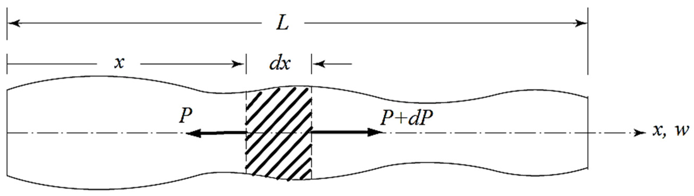
2. Axial Vibration of Rods

Rod vibrations are a fundamental topic in textbooks on mechanical vibrations [35,36,37]. The rod shown in the following figure was considered.
In Figure 1, L is the length of the rod, x is the axial coordinate, w is the axial displacement, and P is the force acting on an infinitesimal element. The governing equation for the free axial vibration of the rod, as shown in Figure 1, is as follows:
x E A ( x ) w ( x , t ) x = ρ A ( x ) 2 w ( x , t ) t 2
Applying the separation of variables techniques with w ( x , t ) = u ( x ) T ( t ) , the governing equation becomes the following:
d d x E A ( x ) d u ( x ) d x + ω 2 ρ A ( x ) u ( x ) = 0
If the cross-sectional area is constant, that is, A(x) = A, Equation (2) takes the following form:
2 u ( x ) x 2 + ω c 2 u ( x ) = 0
where c = E / ρ . Since Equation (3) is a differential equation with constant coefficients, it is much easier to solve than Equation (2).
If the bar is axially functionally graded, then the governing equation reads as follows:
x E ( x ) A ( x ) w ( x , t ) x = ρ ( x ) A ( x ) 2 w ( x , t ) t 2
Applying the separation of variables technique, Equation (4) becomes the following [19]:
d d x E ( x ) A ( x ) d u ( x ) d x + ω 2 ρ ( x ) A ( x ) u ( x ) = 0
If the axial stiffness and density are constant, Equation (5) takes the form given in Equation (3). Equation (5) is now expanded to produce the following equation.
d 2 u ( x ) d x 2 + 1 E ( x ) A ( x ) d d x E ( x ) A ( x ) d u ( x ) d x + ω 2 ρ ( x ) E ( x ) u ( x ) = 0
For homogeneous rods, Equation (6) reduces into a simpler form.
d 2 u ( x ) d x 2 + 1 A ( x ) d d x A ( x ) d u ( x ) d x + ω c 2 u ( x ) = 0
The exact solutions of Equations (6) and (7) are available only for a limited number of cases. This study aimed to provide an analytical-based numerical approach for solving both equations for the computation of free axial vibration frequencies.

3. The Method

In this section, a brief explanation of the proposed technique is given.

3.1. ADM

ADM [33] is a powerful technique for solving linear/nonlinear ordinary/partial differential equations and has attracted significant attention in the applied sciences.
Consider an equation of the following form.
L y + R y + N y = f ( x )
where L is the linear operator of maximum order, N is the nonlinear operator, and R is the operator for the remaining terms. We assume that L is a second-order derivative: i.e., L = d 2 / d x 2 . Then, the inverse operator of L is
L 1 = 0 x 0 t . d τ d t
If all terms on the left-hand side of the equation in Equation (4) are taken to the right-hand side except for term Ly, then, by applying the inverse operator to both sides of the equation, the following relation is obtained:
y ( x ) = y ( 0 ) + x y ( 0 ) + g ( x ) L 1 R y L 1 N y
where g(x) is obtained by integrating function f(x). The solution is defined as follows:
y ( x ) = n = 0 y n ( x )
N y ( x ) = n = 0 A n ( x )
In Equation (8), An(x) is the nth Adomian polynomial and is defined as follows:
A k = 1 k ! λ k N n = 0 y n λ n λ = 0 k = 0 , 1 , 2 ,
Inserting Equations (11) and (12) into Equation (10), the following successive relations are obtained.
y 0 ( x ) = y ( 0 ) + x y ( 0 ) + g ( x )
y k ( x ) = L 1 R y k 1 ( x ) L 1 A k 1 ( x )       k 1
Finally, the solution can be defined in terms of an infinite series as follows:
y ( x ) = lim n k = 0 n y k ( x )
After calculating the N terms, the solution to Equation (16) with these terms is called an Nth-order solution.

3.2. VIM

VIM is an analytical technique used to solve linear/nonlinear ordinary/partial differential equations [32]. This method rapidly converges to accurate results.
We consider the following differential equation:
L y + N y = f ( x )
where L is a linear operator, N is a nonlinear operator, and f(x) is a known non-homogeneous term. VIM proposes a correction function for the solution to Equation (17):
y n ( x ) = y n 1 ( x ) + 0 x λ ( τ ) L y n 1 ( τ ) + N y ˜ n 1 ( τ ) f ( τ )       n 1
where l is a generalized Lagrange multiplier based on variational theory. In addition, y n ( x ) is the nth-order approximation for y(x), and y ˜ n x is a limited variation of the nth-order approximation: that is, δ y ˜ n τ = 0 . Considering the limited variation, if a variation is applied to Equation (18), the following relation is obtained.
δ y n ( x ) = δ y n 1 ( x ) + δ 0 x λ ( τ ) L y n 1 ( τ )
Expanding the parenthesis, the following equation can be written.
δ y n ( x ) = δ y n 1 ( x ) + λ ( τ ) 0 τ L δ y n 1 ( ξ ) d ξ τ = 0 τ = x 0 x λ ( τ ) 0 τ L δ y n 1 ( ξ ) d ξ d τ
By applying stationary boundary conditions to Equation (20), the optimal value of the Lagrange multiplier is obtained. Once the Lagrange multiplier has been determined, the solution to Equation (17) can be calculated using the following successive approximations:
y n ( x ) = y n 1 ( x ) + 0 x λ ( τ ) L y n 1 ( τ ) + N y n 1 ( τ ) f ( τ )       n 1
The initial approximation y0(x) is predefined and is chosen generally as the solution for the linear operator.

3.3. Subdomain-Based Numerical Solution Approach

The rod considered in this study was divided into subdomains, as shown in the figure below.
The governing equation in Equation (6) can be rearranged in the following form:
d 2 u ( x ) d x 2 + S ( x ) S ( x ) d u ( x ) d x + ω 2 m ( x ) S ( x ) u ( x ) = 0
where S ( x ) = E ( x ) A ( x ) and m ( x ) = ρ ( x ) A ( x ) . The governing equation given in the ith domain is shown in Figure 2, which can be written as follows:
d 2 u ( x ) d x 2 + S ( x ˜ i ) S ( x ˜ i ) d u ( x ) d x + ω 2 m ( x ˜ i ) S ( x ˜ i ) u ( x ) = 0
where x ˜ i is in the interval of the ith subdomain and may be performed in different ways. In this study, x ˜ i was assumed to be the axial coordinate of the center of the ith subdomain. Once S ( x ) / S ( x ) and m ( x ) / S ( x ) are calculated at x ˜ i , they are assumed to be constant throughout the subdomain, which leads to a differential equation with constant coefficients. This type of arrangement simplifies the process described in Equations (15) and (21): for a sufficiently fine division of the problem domain, the central properties represent the sufficient properties of the related subdomain.
In addition to Equation (23), two continuity conditions should be satisfied between the two subdomains. We consider the subdomains shown in Figure 2. Between subdomain i and subdomain i − 1 at node i, the continuity conditions are as follows:
u 2 i 1 = u 1 i
u 2 i 1 = u 1 i
Finally, boundary conditions were applied for different end conditions. The boundary conditions for a fixed and free end are given as follows [35,36,37]:
u ( x ) at   fixed   end = 0
d u ( x ) d x at   free   end = 0
With respect to the initial approximation for the solution of Equation (23), each subdomain is described by the following equation, which satisfies the requirements for the initial approximation of VIM and ADM:
u 0 i ( ξ ) = A i + B i ξ
where ξ is the local coordinate. The Nth-order solution is sought within each subdomain according to Equations (15) and (21) based on ADM and VIM, respectively. A second-order solution for subdomain i via ADM with the initial approximation given in Equation (28) reads as follows:
u i 2 ( ξ ) = A i 1 β i ξ 2 2 + α i β i ξ 3 6 + β i 2 ξ 4 24 + B i ξ α i ξ 2 2 + α i 2 ξ 3 6 β i ξ 3 6 + α i β i ξ 4 12 + β i 2 ξ 5 120
where α i = S ( x ˜ i ) / S ( x ˜ i ) and β i = m ( x ˜ i ) / S ( x ˜ i ) . Then, the derivative of the second-order axial displacement with respect to the local coordinate would be as follows:
d u i 2 ( ξ ) d ξ = A i β i ξ + α i β i ξ 2 2 + β i 2 ξ 3 6 + B i 1 α i ξ + α i 2 ξ 2 2 β i ξ 2 2 + α i β i ξ 3 3 + β i 2 ξ 4 24
Continuity conditions given in Equations (24) and (25) can be written with the second-order displacement in Equation (29) as follows:
A i 1 1 β i 1 L i 1 2 2 + α i 1 β i 1 L i 1 3 6 + β i 1 2 L i 1 4 24 + B i 1 ξ α i 1 L i 1 2 2 + α i 1 2 L i 1 3 6 β i 1 L i 1 3 6 + α i 1 β i 1 L i 1 4 12 + β i 1 2 L i 1 5 120 = A i
A i 1 β i 1 L i 1 + α i 1 β i 1 L i 1 2 2 + β i 1 2 L i 1 3 6 + B i 1 1 α i 1 L i 1 + α i 1 2 L i 1 2 2 β i 1 L i 1 2 2 + α i 1 β i 1 L i 1 3 3 + β i 1 2 L i 1 4 24 = B i
where L i 1 = x i x i 1 is the length of the domain i − 1 (see Figure 2). Hence, second-order solutions in subdomains lead to the following relation in matrix form, which is obtained for node i.
1 β i 1 L i 1 2 2 + α i 1 β i 1 L i 1 3 6 + β i 1 2 L i 1 4 24 ξ α i 1 L i 1 2 2 + α i 1 2 L i 1 3 6 β i 1 L i 1 3 6 + α i 1 β i 1 L i 1 4 12 + β i 1 2 L i 1 5 120 1 0 β i 1 L i 1 + α i 1 β i 1 L i 1 2 2 + β i 1 2 L i 1 3 6 1 α i 1 L i 1 + α i 1 2 L i 1 2 2 β i 1 L i 1 2 2 + α i 1 β i 1 L i 1 3 3 + β i 1 2 L i 1 4 24 0 1 A i 1 B i 1 A i B i = 0 0 0 0
The fourth-order solution provides additional terms to the multiples of Ai and Bi given in the parentheses in Equation (29). In this study, second- and fourth-order solutions are used in each subdomain.
After applying all the required continuity and boundary conditions at each node, the following equation in the matrix form is obtained:
K ( ω ) Λ = 0
In Equation (34), [K] is the coefficient matrix, which is a function of free vibration frequency w. {Λ} is a vector composed of coefficients Ai’s and Bi’s. A non-trivial solution to Equation (34) leads to the desired free vibration frequencies.
Below, the proposed approach is applied to a number of case studies available in the literature.

4. Numerical Results

In this section, the proposed technique is applied to available problems in the literature.

4.1. Case 1

Eisenberger [2] calculated the free axial vibration frequencies of a variable cross-section fixed–free rod with two different area functions. Both ADM and VIM are employed in the solution, and the results are compared below with different numbers of subdomains and solution orders within each subdomain. In the table, n represents the number of subdomains, and m represents the order of the solution within each subdomain.
From Table 1 and Table 2, it can be observed that ADM and VIM provide the same answers for each frequency with assumed values of n and m. Hence, from now on, the results of this study will be given as a single value for each of the cases considered. From Table 2, the second-order solution for the first frequency appears to be adequate, whereas for other frequencies, the fourth-order solution is required. The improvement of the solution with the number of subdomains is investigated below for both cases. Hence, the fourth-order solution was used in the solutions. Table 3 and Table 4 show that with a fine mesh, the results obtained using centroidal properties within each subdomain are in perfect agreement with the results in [2]. In conclusion, the proposed approach provides perfect results with the advantage of computation ease.

4.2. Case 2

Kumar and Sujith [5] considered specific cross-sectional area functions to determine the exact longitudinal vibration frequencies of non-uniform rods. However, numerical extraction from analytical expressions was computed incorrectly, and the results for various cases were corrected by other researchers [38,39]. The proposed approach was implemented with fourth-order solutions within each subdomain. The results are given in the tables below.
Table 5, Table 6 and Table 7 show very good agreement between the results of this study and those in [5,39]. Even for the largest mode with n = 20 , the maximum relative error is less than 0.00002. Hence, the proposed approach yields excellent results using the centroidal properties of each subdivision.
Different variations in the cross-sectional area were also considered in the same study [5].
In Table 8, Table 9 and Table 10, the results of this study agree very well with the analytical results [5,41]. The maximum relative error for the square sine function with n = 20 is less than 0.00003. Consequently, the proposed approach worked very well in this case.

4.3. Case 3

Guo and Yang [16] obtained a series solution for a fixed–fixed rod using an exponential area function. The proposed method was applied to the case, and the first five frequencies for fixed–free and free–free rods were also computed for the researchers for further studies on the subject.
As shown in Table 11, the results of this study are in perfect agreement with those in [9]. Guo et al. [9] only considered a fixed–fixed rod. As a contribution, we computed the first five frequencies of the fixed–free and free–free rods for the same area function using 100 subdomains in the solution region. Table 12 presents the results below.

4.4. Case 4

Yardimoglu and Aydin [17] obtained exact solutions for the longitudinal natural vibration frequencies of rods with variable cross-sections. Yardimoglu considered the area function as a power of sine function, that is, s i n n a x + b , and calculated the frequencies of vibrations with different a, b, and n values for different end conditions. Nine different cases were considered [17]. Although the results of all cases in the paper agree very well with the proposed technique, only three of them are provided for comparison purposes. Below, the comparisons were chosen for the fixed values of b = 1 and a = π 2 b , and 100 subdomains were used in the analysis.
As shown in Table 13, Table 14 and Table 15, the largest relative error was less than 2 × 10⁻⁶. The results obtained using the proposed technique agree very well with the analytical solutions [17]. Hence, the applied computational procedure was highly effective in this case.

4.5. Case 5

Shahba et al. [18], Shahba and Rajasekaran [19], and Pillutla et al. [28] studied the longitudinal free vibration of axially functionally graded rods using various computational approaches. They considered a tapered bar with a rectangular cross-section for which its breath taper ratio is cb and height taper ratio is ch, and its cross-section is given by A ( x ) = 1 c b x ¯ 1 c h x ¯ , where x ¯ = x / L . The modulus of elasticity and mass density vary as E = E 0 ( 1 + x ¯ ) and ρ = ρ 0 1 + x ¯ + x ¯ 2 . Numerical experiments showed that 20 subdomains were adequate for the first three frequencies. However, to determine the first six vibration frequencies, 100 subdomains were used in the calculations. In [18,19,28], the first three vibration frequencies of fixed–fixed and fixed–free rods were considered.
The efficiency of the proposed method can be observed in Table 16 and Table 17. Due to the accurate results from the presented approach, additional information is presented in Table 18 and Table 19 for the researchers for further studies on the subject.
In this study, additional computations are conducted for further research. These additional results are given in Table 18 and Table 19 below.

4.6. Case 6

Shahba et al. [20] and Pillutla et al. [28] studied the longitudinal free vibration of axially functionally graded rods with a cross-section given by A ( x ) = 1 c x ¯ , where x ¯ = x / L . The modulus of elasticity and mass density varied according to E = E 0 e x ¯ and ρ = ρ 0 e x ¯ . As in the previous case, the numerical experiments showed that 20 subdomains were adequate for comparison. However, 100 subdomains were used to accurately determine the first six vibration frequencies. The results are summarized in the tables below.
As shown in Table 20, the results obtained from this study are in very good agreement with [28], even with 20 subdomains. However, for further research, additional computations were conducted, and the results shown in Table 21, Table 22 and Table 23 were obtained according to different combinations of boundary conditions.

5. Conclusions

In this study, the axial free vibration of non-uniform, homogeneous, and functionally graded rods is considered. The governing equation of the problem is a variable coefficient differential equation, for which the analytical solutions are strictly limited. Analytical approximate solution methods are available for these types of problems. Although these methods are efficient, the analytical integration process becomes cumbersome or sometimes impossible for higher-order solutions to achieve better convergence. This study aims to propose a subdomain-based numerical solution approach to eliminate difficulties in the integration process while benefitting from the analytical formulation. Several case studies were considered, including polynomial, sinusoidal, and exponential variations of the cross-sectional area, for which the proposed technique led to excellent results. Functionally graded rods with variable cross-sectional areas and variable material properties were also considered. The proposed method was also very effective and yielded very good results. Numerical studies showed that 20 subdomains were sufficient for the first three vibration frequencies, whereas it was also sufficient for the first six vibration frequencies if the variation functions for the cross-sectional areas were not too complex. However, 100 subdomains were preferred for most comparative studies. Because the presented technique provided excellent results, additional computations were conducted for researchers who will aim to consider the problem in future research using different solution methods. In conclusion, the proposed approach is very effective in solving the vibration problems of homogeneous and functionally graded rods with variable cross-sectional areas.

Author Contributions

Conceptualization, S.B.C.; methodology, S.B.C. and K.K.; mathematical modelling S.B.C. and K.K., formal analysis, K.K.; software, K.K.; writing—original draft preparation, S.B.C. and K.K.; writing—review and editing, S.B.C. and K.K.; All authors have read and agreed to the published version of the manuscript.

Funding

This research received no external funding.

Data Availability Statement

Not applicable.

Conflicts of Interest

The authors declare no conflict of interest.

References

  1. Raman, V.M. On analytical solutions of vibrations of rods with variable cross sections. Appl. Math. Model. 1983, 7, 356–361. [Google Scholar] [CrossRef]
  2. Eisenberger, M. Exact longitudinal vibration frequencies of a variable cross-section rod. Appl. Acoust. 1991, 34, 123–130. [Google Scholar] [CrossRef]
  3. Abrate, S. Vibration of nonuniform rods and beams. J. Sound Vib. 1995, 185, 703–716. [Google Scholar] [CrossRef]
  4. Bapat, C.N. Vibration of rods with uniformly tapered sections. J. Sound Vib. 1995, 185, 185–189. [Google Scholar] [CrossRef]
  5. Kumar, B.M.; Sujith, R.I. Exact solutions for the longitudinal vibration of non-uniform rods. J. Sound Vib. 1997, 207, 721–729. [Google Scholar] [CrossRef]
  6. Li, Q.S. Exact solutions for free longitudinal vibrations of non-uniform rods. J. Sound Vib. 2000, 234, 1–19. [Google Scholar] [CrossRef]
  7. Li, Q.S. Exact solutions for free longitudinal vibration of stepped non-uniform rods. Appl. Acoust. 2000, 60, 13–28. [Google Scholar] [CrossRef]
  8. Zeng, H.; Bert, C.W. Vibration analysis of a tapered bar by differential transformation. J. Sound Vib. 2001, 242, 737–739. [Google Scholar] [CrossRef]
  9. Raj, A.; Sujith, R.I. Closed-form solutions for the free longitudinal vibration of inhomogeneous rods. J. Sound Vib. 2005, 283, 1015–1030. [Google Scholar] [CrossRef]
  10. Elishakoff, I. Eigenvalues of Inhomogeneous Structures: Unusual Closed-Form Solutions; CRC Press: Boca Raton, FL, USA, 2005. [Google Scholar]
  11. Al Kaisy, A.M.A.; Esmaeel, R.A.; Nassar, M.M. Application of the differential quadrature method in the longitudinal vibration of non-uniform rods. Eng. Mech. 2007, 14, 303–310. [Google Scholar]
  12. Provatidis, C.G. Free vibration analysis of elastic rods using global collocation. Arch. Appl. Mech. 2008, 78, 241–250. [Google Scholar] [CrossRef]
  13. Calio, I.; Elishakoff, I. Exponential solution for a longitudinally vibrating inhomogeneous rod. J. Mech. Mater. Struct. 2009, 4, 1251–1259. [Google Scholar] [CrossRef]
  14. Arndt, M.; Machado, R.D.; Scremin, A. An adaptive generalized finite element method applied to free vibration analysis of straight bars and trusses. J. Sound Vib. 2010, 329, 659–672. [Google Scholar] [CrossRef]
  15. Inaudi, J.A.; Matusevich, A.E. Domain-partition power series in vibration analysis of variable-cross-section rods. J. Sound Vib. 2010, 329, 4534–4549. [Google Scholar] [CrossRef]
  16. Guo, S.Q.; Yang, S.P. Free longitudinal vibrations of non-uniform rods. Sci. China Technol. Sci. 2011, 54, 2735–2745. [Google Scholar] [CrossRef]
  17. Yardimoglu, B.; Aydin, L. Exact longitudinal vibration characteristics of rods with variable cross-sections. Shock Vib. 2011, 18, 555–562. [Google Scholar] [CrossRef]
  18. Shahba, A.; Attarnejad, R.; Hajilar, S. Free vibration and stability of axially functionally graded tapered Euler-Bernoulli beams. Shock Vib. 2011, 18, 683–696. [Google Scholar] [CrossRef]
  19. Shahba, A.; Rajasekaran, S. Free vibration and stability of tapered Euler-Bernoulli beams made of axially functionally graded materials. Appl. Math. Model. 2012, 36, 3094–3111. [Google Scholar] [CrossRef]
  20. Shahba, A.; Attarnejad, R.; Hajilar, S. A Mechanical-Based Solution for Axially Functionally Graded Tapered Euler-Bernoulli Beams. Mech. Adv. Mater. Struct. 2013, 20, 696–707. [Google Scholar] [CrossRef]
  21. Gan, C.; Wei, Y.; Yang, S. Longitudinal wave propagation in a rod with variable cross-section. J. Sound Vib. 2014, 333, 434–445. [Google Scholar] [CrossRef]
  22. Hong, M.; Parl, I.; Lee, U. Dynamics and waves characteristics of the FGM axial bars by using spectral element method. Compos. Struct. 2014, 107, 585–593. [Google Scholar] [CrossRef]
  23. Shokrollahi, M.; Nejad, A.Z.B. Numerical Analysis of Free Longitudinal Vibration of Nonuniform Rods: Discrete Singular Convolution Approach. J. Eng. Mech. 2014, 140, 06014007. [Google Scholar] [CrossRef]
  24. Guo, S.; Yang, S. Longitudinal vibrations of arbitrary non-uniform rods. Acta Mech. Solida Sin. 2015, 28, 187–199. [Google Scholar] [CrossRef]
  25. Shali, S.; Nagaraja, S.R.; Jafarali, P. Vibration of non-uniform rod using Differential Transform Method. IOP Conf. Ser. Mater. Sci. Eng. 2017, 225, 012027. [Google Scholar] [CrossRef]
  26. Šalinića, S.; Obradović, A.; Tomović, A. Free vibration analysis of axially functionally graded tapered, stepped, and continuously segmented rods and beams. Compos. B. Eng. 2018, 150, 135–143. [Google Scholar] [CrossRef]
  27. Celebi, K.; Yarimpapuc, D.; Baran, T. Forced vibration analysis of inhomogeneous rods with non-uniform cross-section. J. Eng. Res. 2018, 6, 189–202. [Google Scholar]
  28. Pillutla, S.H.; Gopinathan, S.; Yerikalapudy, V.R. Free longitudinal vibrations of functionally graded tapered axial bars by pseudospectral method. J. Vibroeng. 2018, 20, 2137–2150. [Google Scholar] [CrossRef]
  29. Jedrysiak, J. Vibrations of microstructured beams with axial force. Vib. Phys. Syst. 2020, 31, 2020208. [Google Scholar] [CrossRef]
  30. Jedrysiak, J. Theoretical tolerance modelling of dynamics and stability for axially functionally graded (AFG) beams. Materials 2023, 16, 2096. [Google Scholar] [CrossRef]
  31. Zhou, J.K. Differential Transformation and Its Application for Electrical Circuits; Huazhong University Press: Wuhan, China, 1986. (In Chinese) [Google Scholar]
  32. He, J.-H. Variational iteration method—A kind of non-linear analytical technique: Some examples. Int. J. Non-Linear Mech. 1999, 34, 699–708. [Google Scholar] [CrossRef]
  33. Adomian, G. Solving Frontier Problems of Physics: The Decomposition Method; Kluwer Academic Publishers: Dordrecht, The Netherlands, 1994. [Google Scholar]
  34. He, J.-H. Homotopy perturbation method: A new nonlinear analytical technique. Appl. Math. Comput. 2003, 135, 73–79. [Google Scholar] [CrossRef]
  35. Liao, S.J. The Proposed Homotopy Analysis Technique for the Solution of Nonlinear Problems. Ph.D. Thesis, Shanghai Jiao Tong University, Shanghai, China, 1992. [Google Scholar]
  36. Marinca, V.; Herisanu, N.; Marinca, B. Optimal Auxiliary Functions Method for Nonlinear Dynamical Systems; Springer: Cham, Switzerland, 2021. [Google Scholar]
  37. Den Hartog, J.P. Mechanical Vibrations; Dover Publications: Mineola, NY, USA, 1985. [Google Scholar]
  38. Yardimoglu, B. Exact solutions for the longitudinal vibration of non-uniform rods [J. Sound Vib.207(1997)721–729]. J. Sound Vib. 2010, 329, 4107. [Google Scholar] [CrossRef]
  39. Bahrami, A. Comments on “Exact solutions for the longitudinal vibration of non-uniform rods [J. Sound Vib. 1997, 207, 721–729]”. J. Sound Vib. 2019, 442, 843–844. [Google Scholar] [CrossRef]
  40. Kelly, S.G. Mechanical Vibrations: Theory and Applications; Cengage Learning: Boston, MA, USA, 2012. [Google Scholar]
  41. Rao, S.S. Mechanical Vibrations, 6th ed.; Pearson: London, UK, 2017. [Google Scholar]
Figure 1. Rod in axial vibration.
Vibration 06 00052 g001
Figure 2. Subdomains.
Vibration 06 00052 g002
Table 1. Comparison of results via ADM and VIM for A x = 2 x .
n = 10 [2]
First Five
Frequencies
m = 2 m = 4
ADMVIMADMVIM
1.794661.794661.794101.794101.79401
4.802054.802054.802114.802114.80206
7.910277.910277.908997.908997.90896
11.0568811.0568811.0351111.0351111.03509
14.2517114.2517114.1680114.1680114.16799
Table 2. Comparison of results via ADM and VIM for A x = 3 4 x + 2 x 2 .
n = 10 [2]
First Five
Frequencies
m = 2 m = 4
ADMVIMADMVIM
1.970351.970351.970111.970111.97090
4.821924.821924.820584.820584.82076
7.918057.918057.918137.918137.91820
11.0531511.0531511.0413911.0413911.04144
14.2308514.2308514.1728214.1728214.17284
Table 3. Comparison of results with A x = 2 x for a different number of subdomains.
This Study[2]
First Five
Frequencies
n = 10 n = 20 n = 50
1.794101.794031.794011.79401
4.802114.802074.802064.80206
7.908997.908977.908967.90896
11.0351111.0351011.0351011.03509
14.1680114.1679914.1679914.16799
Table 4. Comparison of results with A x = 3 4 x + 2 x 2 for a different number of subdomains.
n = 10 [2]
First Five
Frequencies
m = 2 m = 4
ADMVIMADMVIM
1.970781.970881.970901.970901.97078
4.820714.820754.820764.820764.82071
7.918187.918207.918207.918207.91818
11.0414311.0414411.0414411.0414411.04143
14.1728314.1728414.1728414.1728414.17283
Table 5. Comparison of results for the fixed–fixed rod with A x = a x + b 4 , b = 1 .
Mode a = 1 a = 2
This Study
n = 20
This Study
n = 100
[40]This Study
n = 20
This Study
n = 100
[40]
13.2860293.2860073.2859983.4744863.4743393.474339
26.3607106.3606786.3606716.4802826.4800346.480028
39.4772539.4771969.4771809.5617819.5613709.561367
412.60600212.60589012.60580212.67104812.67036212.670323
515.73988115.73965615.73964815.79290015.79175215.791747
618.87644518.87600218.87453318.92155818.91965518.919130
Table 6. Comparison of results for the fixed–free rod with A x = a x + b 4 , b = 1 .
Mode a = 1 a = 2
This Study
n = 20
This Study
n = 100
[40]This Study
n = 20
This Study
n = 100
[40]
10.8249110.8249690.8249710.5265250.5266860.526694
24.6004694.6004544.6004544.6895034.6893324.689329
37.7891327.7890977.7890967.8490007.8486977.848695
410.94973410.94965910.94965910.99412910.99361210.993610
514.10174614.10159214.10159114.13711114.13623714.136235
617.25002217.24970917.24970817.27971517.27824917.278247
Table 7. Comparison of results for the free–free rod with A x = a x + b 4 , b = 1 .
Mode a = 1 a = 2
This Study
n = 20
This Study
n = 100
[40]This Study
n = 20
This Study
n = 100
[40]
13.5558873.5557923.5557884.0418294.0413404.041322
26.5131496.5130706.5130686.8577666.8571916.857173
39.5813609.5812729.5812709.8306589.8300009.829986
412.68474412.68461012.68460812.87742812.87656312.876551
515.80312015.80287815.80287715.95973315.95846315.958453
618.92925318.92879918.92879819.06134119.05936819.059359
Table 8. Comparison of results for fixed–fixed rod with A x = A 0 sin 2 a x + b , b = 1 .
Mode a = 1 a = 2
This Study
n = 20
This Study
n = 100
[40]This Study
n = 20
This Study
n = 100
[40]
12.9781512.9781872.9781892.4228272.4226012.422727
26.2030796.2030976.2030975.9554215.9562565.956376
39.3715659.3715769.3715769.2101529.2100089.210127
412.52651312.52651812.52651912.40730512.40608012.406195
515.67610315.67610015.67610015.58235715.58001215.580119
618.82303318.82301118.82301118.74655718.74305418.743152
Table 9. Comparison of results for fixed–free rod with A x = A 0 sin 2 a x + b , b = 1 .
Mode a = 1 a = 2
This Study
n = 20
This Study
n = 100
[40]This Study
n = 20
This Study
n = 100
[40]
11.5176231.5176371.5176382.1494262.1485932.148560
24.7021424.7021454.7021455.5398525.5359225.535762
37.8483107.8483117.8483118.6399368.6330938.632812
410.99162110.99162110.99162011.70383311.69501411.694640
514.13412814.13412314.13412014.76799114.75828814.757860
617.27629717.27682417.27628017.84071917.83105417.830600
Table 10. Comparison of results for free–free rod with A x = A 0 sin 2 a x + b , b = 1 .
Mode a = 1 a = 2
This Study
n = 20
This Study
n = 100
[40]This Study
n = 20
This Study
n = 100
[40]
13.3091093.3090713.3090704.2124064.2097144.209604
26.3752336.375096.3752097.2657567.2600927.259860
39.4873809.4873639.48736310.29190210.28383610.283498
412.61366312.61364912.61364813.32782213.31838813.317980
515.74593015.74591415.74591316.37916216.36936616.368917
618.88127118.88124018.88124019.44517719.43580119.435335
Table 11. Comparison of results for the fixed–fixed rod with A x = A 0 e c x 2 / L 2 , L = 1 .
Mode c = 0.5 c = 1 c = 2
This Study
n = 100
Kummer Function [16]This Study
n = 100
Kummer Function [16]This Study
n = 100
Kummer Function [16]
13.2311302813.2311302813.3393358673.3393358673.6031397933.603139793
26.3291866756.3291866756.3874402556.3874402546.5395626856.539562675
39.4556003579.4556003579.4949640599.4949640589.5989804489.598980427
412.5895281912.5895281912.6191902212.6191902212.6978867412.69788671
Table 12. First five frequencies of fixed–free and free–free rods with A x = A 0 e c x 2 / L 2 , L = 1 .
Mode c = 0.5 c = 1 c = 2
Fixed–FreeFree–FreeFixed–FreeFree–FreeFixed–FreeFree–Free
11.4142143.0724911.2636933.0250890.9858862.997101
24.6673696.2496884.6387126.2289164.6317316.226225
37.8272829.4025737.8109229.3890547.8096089.388313
410.97656412.54975010.96503612.53969510.96457612.539391
514.12240115.69467914.11348415.68666614.11327115.686512
Table 13. Comparison of results for the fixed–fixed rod with A x = A 0 sin n a x + b .
Mode n = 1 n = 2 n = 3 n = 4
This Study[17]This Study[17]This Study[17]This Study[17]
13.0336563.0336582.9268342.9268362.8212422.8212462.7169982.717003
26.2284746.2284756.1786066.1786076.1336946.1336966.0938376.093840
39.3881719.3881719.3553839.3553849.3264559.3264569.3014239.301424
412.53887712.53887712.51440912.51440912.49298412.49298512.47462012.474621
515.68595315.68595415.66642515.66642515.64938715.64938715.63484815.634849
618.83120818.83120818.81495418.81495518.80080218.80080318.78875718.788757
Table 14. Comparison of results for the fixed–free rod with A x = A 0 sin n a x + b .
Mode n = 1 n = 2 n = 3 n = 4
This Study[17]This Study[17]This Study[17]This Study[17]
11.5681231.5681231.5601541.5601551.5470411.5470411.5290221.529023
24.7158304.7158304.7261034.7261024.7430644.7430644.7664854.766484
37.8563727.8563727.8635377.8635377.8754597.8754597.8921097.892108
410.99735010.99735011.00267811.00267811.01155211.01155211.02396811.023967
514.13857114.13857114.14278314.14278314.14980114.14980114.15962414.159624
617.27991817.27991817.28339217.28339217.28918317.28918317.29728817.297288
Table 15. Comparison of results for the free–free rod with A x = A 0 sin n a x + b .
Mode n = 1 n = 2 n = 3 n = 4
This Study[17]This Study[17]This Study[17]This Study[17]
13.2505243.2505233.3603313.3603283.4708953.4708913.5820983.582093
26.3426116.3426106.4066076.4066056.4750186.4750156.5476796.547675
39.4651609.4651609.5092709.5092699.5570589.5570569.6084699.608466
412.59687112.59687012.63035612.63035512.66680712.66680512.70619912.706197
515.73244415.73244415.75938615.75938515.78877615.78877715.82060715.820605
618.86999418.86999318.89251518.89251418.91711218.91711318.94378218.943781
Table 16. Comparison of results for fixed–fixed functionally graded rods.
chcb ω 1 ω 2 ω 3
[19][28]This Study[19][28]This Study[19][28]This Study
0.00.02.8760-2.8759635.7627-5.7627208.6453-8.645279
0.22.8631-2.8631245.7562-5.7561978.6409-8.640920
0.42.8415-2.8414615.7453-5.7453208.6337-8.633663
0.62.8023-2.8023355.7251-5.7251088.6201-8.620077
0.82.7192-2.7192005.6767-5.6766348.5860-8.586022
0.20.22.85392.8539262.8539225.75155.7515015.7514938.63788.6378418.637772
0.42.83692.8369362.8369335.74305.7429575.7429668.63218.6321478.632078
0.62.80422.8042232.8042185.72605.7260235.7260148.62078.6207478.620682
0.82.73112.7311192.7311075.68295.6828855.6829008.59038.5903378.590280
0.40.42.82602.8259732.8259705.73755.7374985.7374898.62848.6285048.628435
0.62.80162.8015612.8015575.72495.7249295.7249208.62008.6200568.619992
0.82.74152.7415192.7415085.68925.6891705.6891568.59478.5947488.594692
0.60.62.78862.7886442.7886405.71885.7187755.7187658.61608.6159998.615940
0.82.74682.7468132.7468035.69425.6942045.6941928.59868.5986318.598578
0.80.82.73402.7340412.7340305.69015.6900565.6900568.59658.5965218.596473
Table 17. Comparison of results for fixed–free functionally graded rods.
chcb ω 1 ω 2 ω 3
[19][28]This Study[19][28]This Study[19][28]This Study
0.00.01.1901-1.1901214.2549-4.2549087.1650-7.165005
0.21.2503-1.2502734.2683-4.2683437.1728-7.172861
0.41.3293-1.3292604.2903-4.2902917.1859-7.185878
0.61.4400-1.4400314.3333-4.3332947.2123-7.212325
0.81.6129-1.6128894.4444-4.4443897.2891-7.289126
0.20.21.31191.3119361.3119414.28414.2841334.2841527.18217.1818037.182161
0.41.39281.3927891.3927944.30904.3090444.3090637.19707.1967157.197021
0.61.50591.5059251.5059314.35594.3559434.3559627.22607.2257737.225995
0.81.68181.6818401.6818364.47264.4726464.4726227.30687.3067037.306799
0.40.41.47591.4758711.4758774.33774.3377224.3377407.21437.2140227.214275
0.61.59171.5916951.5917014.38974.3896904.3897087.24667.2464507.246626
0.81.77061.7706681.7706634.51384.5138274.5138017.33297.3329187.332981
0.60.61.71041.7104431.7104504.44874.4486714.4486907.28397.2837917.283910
0.81.89181.8918201.8918144.58324.5832824.5832497.37877.3787287.378747
0.80.82.07232.0723032.0722864.73284.7329204.7328137.48887.4889527.488819
Table 18. Additional non-dimensional frequencies for the functionally graded rod.
chcbFixed–Fixed RodFixed–Free Rod
ω 4 ω 5 ω 6 ω 4 ω 5 ω 6
0.00.011.52738914.40939517.29136410.05850112.94677615.832722
0.211.52411714.40677617.28918110.06407612.95110015.836256
0.411.51867314.40242117.28555210.07334912.95830415.842147
0.611.50845114.39423117.27872010.09238812.97316315.854326
0.811.48230314.37305217.26094310.15017513.01921915.892511
0.20.211.52175314.40488417.28760410.07068712.95623115.840450
0.411.51748114.40146617.28475610.08128612.96447115.847190
0.611.50890614.39459517.27902410.10217112.98077815.860559
0.811.48552914.37564617.26311210.16298413.02924615.900742
0.40.411.51475014.39928217.28293610.09362312.97407115.855046
0.611.50839914.39419417.27869210.11699012.99233115.870023
0.811.48891314.37838517.26540910.18204213.04419215.913024
0.60.611.50537514.39178017.27668310.14403913.01350815.887408
0.811.49200214.38092817.26756410.21571613.07071715.934868
0.80.811.49066814.37997017.26682110.30014913.13851715.991278
Table 19. Non-dimensional frequencies for the free–free functionally graded rod.
chcb ω 1 ω 2 ω 3 ω 4 ω 5 ω 6
0.00.02.9466815.7949618.66627811.54302914.42188317.301774
0.22.9340155.7886838.66211211.53991014.41939017.299698
0.42.9336735.7888208.66225211.54002814.41948917.299782
0.62.9621145.8054458.67371711.54873414.42649417.305639
0.83.0685015.8806398.72910911.59204514.46188217.335486
0.20.22.9248995.7842148.65915611.53769914.41762417.298227
0.42.9291505.7866848.66085411.53898714.41865917.299092
0.62.9637295.8065508.67450311.54933614.42698217.306047
0.83.0785135.8868908.73350111.59540214.46459217.337756
0.40.42.9392815.7922058.66460011.54181414.42092717.300985
0.62.9816025.8163798.68118311.55438014.43103017.309426
0.83.1066495.9036958.74518411.60430114.47176317.343756
0.60.63.0338525.8467738.70210411.57025314.44379617.320096
0.83.1712145.9443708.77381911.62620914.48945317.358572
0.80.83.3209736.0589198.85994711.69396114.54492717.405400
Table 20. Comparison of results for functionally graded rod.
cModeFixed–Fixed RodFixed–Free Rod
[20][28]This Study
n = 20
[20][28]This Study
n = 20
0.113.17573.1724093.1724091.2988 1.29851.298593
26.32476.2986486.2986484.64784.6374244.637424
39.52289.4350939.4350957.85927.8095057.809506
0.313.15143.1481533.1481531.37221.3719581.371958
26.31236.2863656.2863654.66564.6551184.655118
39.51449.4268859.4268857.86987.8199427.819942
0.513.11203.1088313.1088181.47101.4706761.470698
26.29166.2659186.2659114.69834.6875284.687538
39.50059.4131359.4131317.88997.839577.839577
0.812.97802.9752212.9749251.71681.7162511.716528
26.21136.1865686.1863394.84864.8367784.837135
39.44279.3570799.3569097.99587.94334647.943773
Table 21. Non-dimensional frequencies for fixed–fixed rod.
c ω 1 ω 2 ω 3 ω 4 ω 5 ω 6
0.13.1724096.2986489.43509312.57410915.71415418.854715
0.33.1481546.2863669.42688512.56794815.70922318.850605
0.53.1088316.2659189.41313512.55760215.70093518.843693
0.73.0376526.2258629.38551312.53659615.68401318.829536
0.92.8658056.1073389.29487012.46344115.62284718.777080
Table 22. Non-dimensional frequencies for fixed–free rod.
c ω 1 ω 2 ω 3 ω 4 ω 5 ω 6
0.11.2985934.6374247.80950510.96390214.11256317.258642
0.31.3719584.6551187.81994210.97132314.11832417.263351
0.51.4706784.6875297.83957110.98538614.12927717.272319
0.71.6143994.7600557.88697711.02026114.15676517.294968
0.91.8533564.9871538.07617311.17728814.28929517.408893
Table 23. Non-dimensional frequencies for free–free rod.
C ω 1 ω 2 ω 3 ω 4 ω 5 ω 6
0.13.1741576.2995309.43568212.57455115.71450818.855010
0.33.1681216.2965329.43368712.57305515.71331218.854014
0.53.1827586.3048729.43940412.57738715.71679418.856923
0.73.2469296.3463209.46896612.60016115.73525518.872421
0.93.4580606.5386479.63047012.73612915.85149418.973406
Disclaimer/Publisher’s Note: The statements, opinions and data contained in all publications are solely those of the individual author(s) and contributor(s) and not of MDPI and/or the editor(s). MDPI and/or the editor(s) disclaim responsibility for any injury to people or property resulting from any ideas, methods, instructions or products referred to in the content.

