Linear Control of a Nonlinear Equipment Mounting Link

Abstract

The linear control of a nonlinear response is investigated in this paper, and a nonlinear model of the system is developed and validated. The design of the control system has been constrained based on a suggested application, wherein mass and expense are parameters to be kept to a minimum. Through these restrictions, the array of potential applications for the control system is widened. The structure is envisioned as a robot manipulator link, and the control system utilises piezoelectric elements as both sensors and actuators. A nonlinear response is induced in the structure, and the control system is employed to attenuate these vibrations which would be considered a nuisance in practical applications. The nonlinear model is developed based on Euler–Bernoulli beam theory, where unknown parameters are obtained through optimisation based on a comparison with experimentally obtained data. This updated nonlinear model is then compared with the experimental results as a method of empirical validation. This research offers both a solution to unwanted nonlinear vibrations in a system, where weight and cost are driving design factors, and a method to model the response of a flexible link under conditions which yield a nonlinear response.

1. Introduction

A vast amount of research is dedicated to the control of linear vibrations in structures, answering a multitude of questions that this field of research poses. However, whilst there is a large amount of research that concerns nonlinear vibrations and their control, by the very nature of these nonlinear vibrations, there are still many solutions yet to be found. Acknowledging this and considering the evolution of robots and to some extent drones, this research aims to amalgamate the fields of robotics and vibration control. A suggested application for the solution developed in this research pertains to the vibration control of a flexible robot link (or equipment armature) to be envisioned as an additional or replacement link of a robot manipulator mounted on a drone. This suggested application is drawn from previous research [1], wherein the flexible link is purposefully long and thin so it may be used in the exploration of small crevasses during search and rescue missions. In previous work, the response of the link was assumed to be linear; however, in this paper the flexible link is subjected to large deformations and hence geometric nonlinearity is considered.

The geometry of the link lends to its flexibility, which in turn causes a tendency for it to experience unwanted or nuisance vibrations. Whilst an adjustment to the geometry of the link may reduce this tendency, this may render the link impractical for the suggested application as it may be too large for exploration or too heavy for the drone. Hence, a solution to the reduction of nuisance vibrations is sought, specifically the nonlinear response of the link, as the reduction of a linear response has previously been investigated. Given the constraints imposed by the suggested application (which may also be present in others), the hardware of the control system needs to be selected with the total mass kept to a minimum. Piezoelectric elements are renowned within vibration control due to their relatively high force output to mass ratio, and they have been previously used as sensors [2,3], actuators [4,5], and self-sensing actuators [6,7,8]. They have also been used in different categories of vibration control as in passive [9,10,11], semi-passive [12,13], and active [14,15,16]. The former two were not considered as a solution within this research, as a passive vibration control system requires tuning so that it is of the same natural frequency as the structure being controlled, which is impractical and in some cases less effective than active vibration control (AVC). Hence the choice of AVC in this research for the control of a nonlinear response.

The ‘brain’ of the operation, as proven effective in other research, is a single board computer (SBC): the Raspberry Pi 3B+ (RPi). A comparison between alternate SBCs was previously undertaken, and this model was chosen based on its mass, processing capacity, and methods of peripheral connections. Previous research by Iwaniec et al. [17] used a RPi to develop a vibration spectrum analyser. This model was also used by Mahmud et al. [3] alongside lead zirconate titanate (PZT) elements for the purpose of structural health monitoring (SHM). The authors, recognising that the RPi is unable to directly read analogue signals, employed an analogue to digital converter (ADC), and this solution has been utilised in this research.

Previous research has proven the selection of components effective in the reduction of nuisance linear vibrations. The weight and cost of the designed control system was considered advantageous with regards to the suggested application. However, as in other scenarios and applications, the flexible equipment armature may experience nonlinear vibrations which lends to the requirement to investigate the designed control system’s capabilities further. The approach to the control of nonlinear vibrations varies among existing research, with many employing a nonlinear control scheme which can adapt to or be designed for uncertainties in the model of the system. Platanitis and Strganac [18] utilised an adaptive control scheme to account for uncertainties in the model of a nonlinear wing section. They employed AVC on this wing section to control the pitch and plunge through the alteration of the deflection of the leading and trailing edge devices. Research by Khorrami et al. [19] sought to control the vibrations experienced by a two link flexible robot manipulator, again employing an adaptive control with a proportional derivative (PD) inner loop that involved input pre-shaping.

Acknowledging that nonlinear control is effective, it can be a less favourable option in comparison to linear control schemes with the consideration of the requirements for their implementation. This statement is paraphrased from the work by Schweickhardt and Allgöwer [20], and in this work, the authors investigated the implementation of linear control on a nonlinear system. The research implied that the mathematical definition of a ‘linear’ and a ‘nonlinear’ system may not be the only method of distinguishing between the two, and that the classification of a system is not binary. Instead, based on the work and the subsequently coined term “nonlinear measures” by Desoer and Wang [21], a system may be defined as being somewhere in the spectrum between linear and nonlinear. These nonlinear measures are based on the representation of a nonlinear system by both a linear model and an error system, wherein a smaller error gain would result in the higher performance of a linear control scheme on a nonlinear system. An inference may be made that the linear control of a ‘weakly’ nonlinear system will result in an acceptable level of attenuation of nuisance vibrations. In this research, another factor considered in the selection of the control scheme is the processing capacity of the SBC; hence, the control scheme employed is of low complexity.

Whilst the employment of a linear control scheme negates the necessity for the development of a model of the system for use in the experimental investigations, a model for the prediction of the response is vital. An accurate representation of the system would provide further insight and reduce the time taken in further investigations. Previous research investigated a method of determining the unknown parameters in a nonlinear system known as equivalent dynamic stiffness mapping (EDSM) [22]. Two systems were considered in this research, a discrete three degrees of freedom (DOF) Duffing system and a cantilever beam with a nonlinear restoring force applied on its free end. To acquire the dynamics of the nonlinear systems, the modified complex averaging technique (MCXA), finite element modelling (FEM), and arc-length continuation were utilised. A previously developed optimisation based framework (OBF) [23] was also employed on the cantilever beam, where the results were compared with those from the EDSM technique. It was found that the EDSM techniques were sensitive to any inaccuracies, but the resultant response may be employed as the initial parameter estimate for the OBF, lending to a more accurate representation of the response.

In this research, the components of the designed control system are presented, along with the structure, experimental set-up, and experimental technique. The uncontrolled and controlled nonlinear responses of the flexible link are compared, presented, and analysed in terms of the effectiveness of the control system. An analytical model is then developed, utilising the MCXA alongside the arc-length continuation method to obtain the steady state response of the system. Finally the results of the analytical model are compared with the experimental results and are analysed based on the accuracy of the representative model.

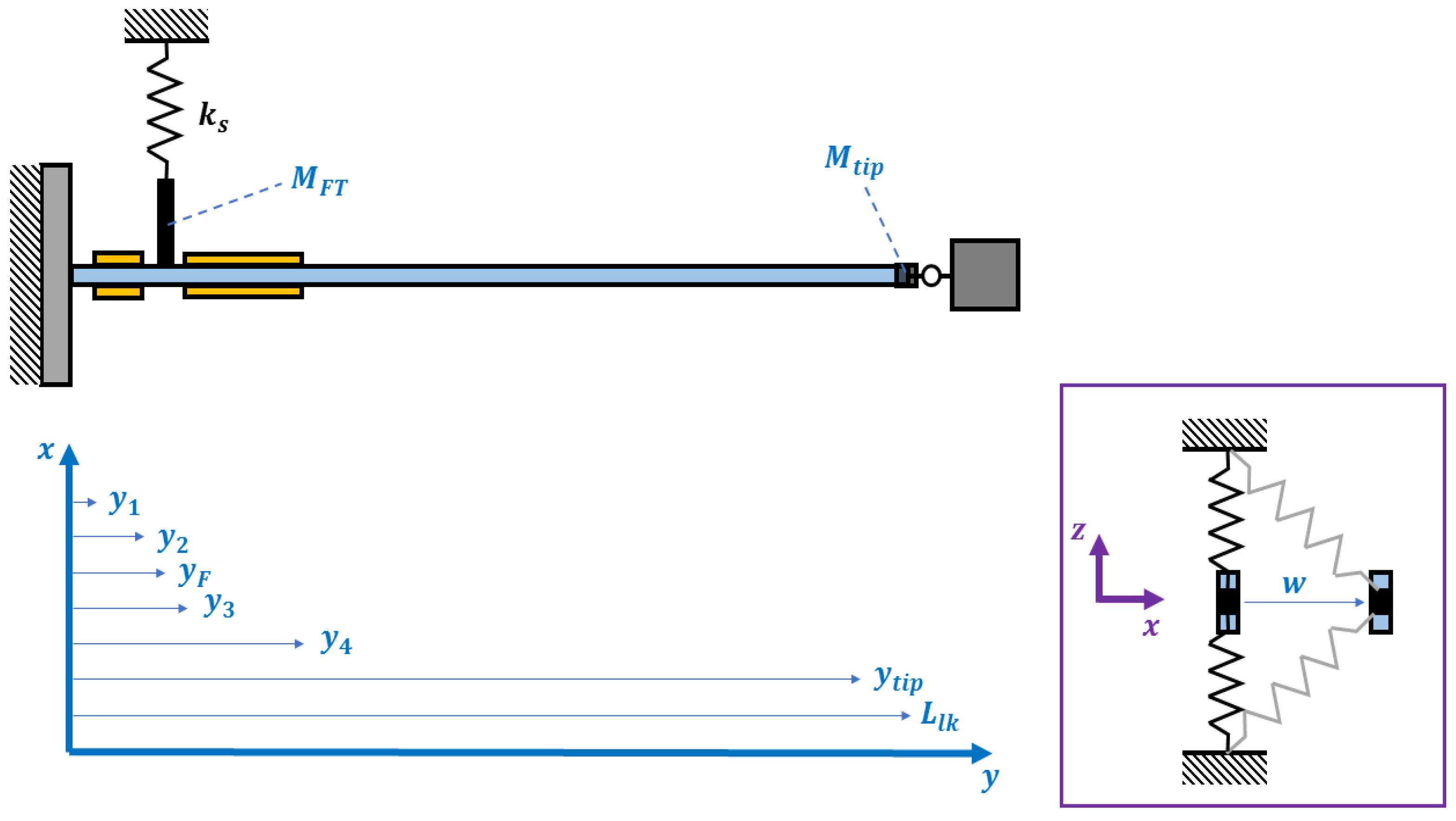
2. Experimental Set-Up

Within this research, the link under experimental investigation was clamped at one end and attached to two springs to induce a geometric nonlinearity. The experimental set-up used is shown in Figure 1, and the components/hardware within this image are numbered as follows:

1.

Shaker (Dataphysics V4);

2.

Force sensor (ICP 208 B02);

3.

Clamp and hinge structure connecting beam to force sensor;

4.

PZT elements;

5.

Springs;

6.

Spring bracket;

7.

Laser displacement sensors (LDSs).

The springs utilised in this set-up have a relaxed length of 0.03728 m and are pre-extended to a length of 0.03769 m (measured using a digital calliper). This pre-extension was employed based on similar research by Shaw et al. [24]. A pre-extension of the springs allowed for a sufficient level of inclusion of both the linear and nonlinear stiffness terms of the spring structure. There are several pieces of the set-up not shown in Figure 1, which includes the data acquisition system (ABACUS 901) connected to a personal computer (PC) and utilised to control the shaker via a SignalForce power amplifier. Also excluded from the image are the direct current (DC) power supply unit for the laser displacement sensors (LDSs) and the majority of the hardware of the designed control system.

The control system employs two sets of collocated PZT elements, one set as actuators and the other as sensors, to control the transverse motion of a flexible link. These PZT elements are surface mounted to the link near the clamped end (see Figure 2), as this has previously been proven to produce the most effective control for the boundary conditions of ‘clamped-free/clamped-supported’ [4]. From Figure 2, the distances along the length of the link ($L_{lk}$) are as follows: $y_1=0.011$ m (start of the sensors), $y_F=0.0223$ m (force application position), $y_3=0.0295$ m (start of actuators), and $y_{tip}=0.257$ m (the measurement position of the transverse displacement). The force is applied parallel to the x axis of Figure 2, and the transverse displacement is also along this axis, which is parallel to the thickness of the link. The stiffness of the stinger structure is represented by $k_s$, the mass of the force transducer and stinger structure is denoted as $M_{FT}$, and the mass at the tip of the link is $M_{tip}$. The geometric, mechanical, and electrical properties of the link, PZT sensors, and PZT actuators are shown in

Table 1. Geometric, mechanical and electric properties of link B and piezoelectric patches [1].

Parameters	Link (Steel)	Piezoelectric Sensor (PZT-5A)	Piezoelectric Actuator (PZT-5A)
Overall length (m)	0.272	0.016	0.066
Overall width (m)	0.0397	0.016	0.031
Thickness (m)	0.0004	0.0003	0.0003
Active length (m)	-	0.007	0.056
Active width (m)	-	0.014	0.028
Density (kg/m${}^3$)	7844	5440	5440
Young’s modulus (GPa)	204	60.48	60.48
Piezoelectric coefficient, ${\overline{e}}_{31}$	-	−11.6	−11.6
Electromechanical coupling term, k	-	0.34	0.34
Capacitance (nF)	-	7.89	113.06

, from which the other distances along the link may be obtained ($y_2$ and $y_4$). It should be noted that the PZT elements have ‘active’ dimensions, which refer to the geometry of the elements that contain PZT material, as the coating on the elements extends beyond this. It is important to distinguish between these two dimension definitions within the analytical model, as the active dimensions should be utilised in the electro-mechanical modelling of the elements and the extended dimensions in the dynamic modelling of the structure.

Two constraints of the RPi required addressing in this research: the SBC is unable to interpret analogue signals and is unable to produce voltages greater than 3.3 V. The solution used to overcome the former of these issues was to employ an analogue to digital converter (ADC): in this case, an MCP3008. However, as with similar ADCs that meet the main requirements of the designed control system to be lightweight and inexpensive, the MCP3008 can only interpret voltages between 0 V and +5 V. Hence, the bipolar analogue signals from the PZT sensors that reached voltages greater than 5 V needed to be adjusted prior to reaching the ADC. Thus, a half wave rectifier circuit (HWRC) and a potential divider circuit (PDC) were employed to prevent the negative and high voltages from reaching the ADC, respectively. These circuits are shown in Figure 3 for one PZT sensor, although it should be noted that the ADC receives the signals from both sensors on different channels, and only one RPi is employed. The HWRC consists of one resistor ($R_1=10$ M$\Omega$) and one diode (1N4184), and the PDC contains two resistors ($R_2=470$ k$\Omega$ and $R_3=1$ M$\Omega$). A visualisation of the rectification of the voltage signals by the HWRC and PDC can be seen in Figure A2 (in Appendix A.2) for arbitrarily selected voltage signals. The RPi corrects the amendments made to these signals so that the amplitude of the voltages used as an input to the control scheme is an accurate representation of the output from the sensors.

The second issue with the RPi was addressed through the inclusion of high voltage drivers (HVDs). These HVDs (DRV2700EVM-HV500) are capable of amplifying a voltage signal to +500 V (the minimum being 0 V). They are lightweight and relatively inexpensive, and their typical use is to apply voltage to PZT elements, making them ideal for this application. However, it should be noted that the PZT actuators have an operating voltage of −60 V to +360 V, and with the positive range in this case being higher, it was chosen for use. The HVDs were then limited to a range of 0 V to +350 V within the control scheme to allow for any spurious voltages that may have been generated by the PZT sensors to protect the PZT actuators from being exposed to voltages higher than their operating range.

With only the positive voltages being read from and applied to the PZT sensors and actuators, respectively, the sensors and actuators were paired. Given the boundary conditions as shown in Figure 1, the sensor on one side of the link was paired with the actuator on the same side. The magnitude of the voltage output from the sensor ($V_{ps}$) controlled the magnitude of the voltage to the actuator ($V_{pa}$) after a proportional gain ($K_p$) was applied to the sensor voltage ( Equation (1)). The control scheme is linear, and its use may be justified based on existing works, as in those previously mentioned [20,21]. An additional source of justification lies in the work by Rudenko and Hedberg [25], wherein the authors highlight that assumptions made in the linearisation of ‘weakly’ nonlinear systems are not applicable to ‘strongly’ nonlinear systems based on the following:

1.

“If the equation of state contains a singularity”.

2.

“If the series diverges for strong disturbances”.

3.

“If the linear term is absent, and higher nonlinearity dominates”.

The system in this research falls within the category of systems which may be described as ‘weakly’ nonlinear; hence, a linear control scheme may be employed (as in Equation (1)).

$$V_{pa}=K_p{V}_{ps}$$

(1)

3. Experimental Results

3.1. Verification of a Nonlinear Response

Prior to the application of control, the experimental set-up was verified to ensure that a nonlinear response was present. A multitude of investigations ensued, here divided into two sets of results, relating to the first (see Figure 4) and second (see Figure 5) resonance frequencies of the structure. The force was applied sinusoidally to the link with a constant magnitude, and the frequency of the motion was swept both upwards and downwards through ranges surrounding the first and second resonance frequencies. Within each set of data, there are subsets that investigate the response of the structure with different magnitudes of force applied; within these subsets, the response due to the sweeping upwards and downwards through the frequencies is shown.

The levels of force in both sets ranged from 3 N to 7 N, and it was found that below this range of force, the response showed nonlinear softening (see Figure A1). This was attributed to some part or parts of the set-up that yield the softening response only at lower force levels. The results obtained for the 3 N force case appear to show a linear response, and the application of higher magnitudes of force yields a pattern inferring nonlinear hardening. Acknowledging these results, and the dedication only to the control of a nonlinear response, any forces lower than 3 N were disregarded (more information can be found in Appendix A.1). Higher force cases than 7 N are also not presented here, and an attempt at investigating the responses as a result of these forces was made, but the integrity of the structure was compromised. As a sufficient response was obtained to investigate the designed control system’s effectiveness with regard to the control of a nonlinear response, it was deemed unnecessary to risk further investigations into higher levels of force.

The first set of results pertaining to the first resonance frequency (Figure 4) is indicative of a system that contains a nonlinear element. The 3 N and 4 N force cases may be empirically considered linear, and by contrast, the 5 N, 6 N, and 7 N cases contain varying degrees of nonlinear characteristics. The latter three cases boast discrepancies in the resonance frequencies of the responses within the comparison of increasing (‘Sweep Up’) and decreasing (‘Sweep Down’) frequencies. This discrepancy is not apparent in either the 3 N or 4 N cases, but is more noticeable in the 7 N case than the 5 N case. This is one indication that nonlinear hardening is present; another is the presence of a ‘jump’ between data points within the sets. Again, this is more apparent in the 7 N case than in the 5 N equivalent, but still present, nonetheless, which is again in support of the presence of nonlinear hardening.

Figure 5 contains the data set of the second resonance frequency investigations; again, the subsets are related to the different magnitudes of force applied—3 N to 7 N—with each subset containing the response from both increasing and decreasing the frequency of the force applied. From the results presented, it can be seen that no nonlinear response is present for these force cases. Given the risk to the integrity of the structure and to some extent the health and safety considerations associated with the application of a higher force level, no further investigations were undertaken. Previous research has proven the designed control system as an effective solution for the attenuation of nonlinear vibrations. Hence, the control of the second mode of the structure is not investigated in depth here; however, this mode is still considered in the investigation of control spillover.

3.2. The Application of Control

To obtain the value of proportional gain that may be considered as the most effective in this research, multiple values were investigated. It was empirically determined from the observation of the results that the most effective value of proportional gain was $K_p=600$. Figure 6a,b contain the resultant response of the system for the cases of 3 N and 7 N excitation force with increasing values of proportional gain, respectively, where it can be seen that the largest reduction in the response amplitude is attained when $K_p=$ 600 for the 3 N force amplitude case. For the 7 N case, there is no improvement or deterioration of the reduction for proportional gain values higher or lower than $K_p=$ 600; hence, it was determined to be the most effective value for use across all three force cases. These three cases of force were 3 N, 5 N, and 7 N, which were applied to the link structure for an excitation frequency range surrounding the first resonance frequency. For each of these force cases, the resultant responses with the application of control for three values of proportional gain ($K_p=$ 0, 100, and 600) are presented in Figure 7a–c. For each of these gains, in turn, two sets of results are included, one pertaining to the response of the system as the frequency of excitation is increased and another when it is decreased.

Figure 7a contains the responses of the structure subject to a 3 N force excitation for the three values of proportional gain. This response is linear, and the designed control system has previously proven effective in attenuating such a response. The results presented here corroborate this. The controlled case where $K_p=100$ shows a reduction in the amplitude of the response by almost a factor of two when compared with the uncontrolled case ($K_p=0$). A further reduction (by approximately a factor of three) can be observed from the results of the controlled case where $K_p=600$. From these results, a discrepancy is also noticeable between the ‘Sweep Up’ and ‘Sweep Down’ data sets with regard to the response amplitude. This was not attributed to the application of control, as there is a variation between these data sets for the uncontrolled case. The alteration of the resonance frequency with the application of control is, however, accredited to the control system, as previous investigations yielded an explanation of this when considering the governing electro-mechanical equations of the PZT sensors. These equations described the output from the PZT sensors as being dependent on the resistance and capacitance within the control system circuitry and hardware, which in turn yielded a response more akin to proportional-derivative (PD) control.

Figure 7b,c contain the results pertaining to the responses where a 5 N and 7 N constant force amplitude were applied, respectively. The response in both of these cases contains characteristics that are indicative of a nonlinear element being present in the structure. These characteristics are more discernible in the 7 N case and remain so even with the application of control, in comparison to the 5 N case. It can be seen that characteristic ‘jumps’ in the data are present in the 5 N uncontrolled case, as is a discrepancy in the resonance frequency (see Figure 7b). With the application of control, the response from a 5 N force excitation contains fewer jumps when $K_p=100$, and apparently none in the case where $K_p=600$. Additionally the difference between the resonance frequencies for the ‘Sweep Up’ and ‘Sweep Down’ data sets is reduced as the proportional gain values is increased. As with the 3 N force case (Figure 7a), the increase in proportional gain is shown to reduce the amplitude of the response, with $K_p=600$ attaining a reduction by an approximate factor of two.

The analysis of the 7 N force case results (Figure 7c) resonates with the findings of the 5 N results with regards to the nonlinear characteristics and the amplitude of the response. The jumps between data sets are reduced with the increase of the proportional gain value, and the discrepancy between the resonance frequencies is also reduced. However, these reductions are noticeably less than those shown in the 5 N case, which may be attributed to the limitations of the PZT actuators in terms of their force output. As the excitation force is increased, the actuators become less able to overcome the transverse motion experienced by the link. However, even with the lesser reduction in the nonlinear characteristics and the amplitude of the response for the highest level of force considered here, the application of the control system can still be considered as an effective solution for the attenuation of the nonlinear response with regards to the first mode of the structure.

A concern with the application of control on the structure in this case lies with the effects of control spillover. If the control system is found to negatively impact the response with regard to the second mode (i.e., increasing the amplitude of the response or inducing a response with nonlinear characteristics), then it may not be considered an effective solution in the attenuation of unwanted vibrations. The results shown in Figure 8a–c consider the response of the structure at frequencies surrounding both the first and second resonance frequencies for the force cases 3 N, 5 N, and 7 N, respectively. It should be noted that the results are presented using a different style for the 3 N case to best reflect the response, as no nonlinear characteristics were found to be present. These results were obtained by sweeping upwards through the frequency range surrounding the first and second resonance frequencies. The responses from sweeping downwards through these frequencies have been disregarded, as the results for the first mode are presented in Figure 7a–c, and the second mode has a linear response at the force levels applied. From Figure 8a–c, it can be seen that the control spillover shows no undesirable effects; in contrast, the control system is shown to reduce the amplitude of the response for all three force cases. Hence, the system may still be considered an effective solution for the reduction of unwanted vibrations.

4. Analytical Model

4.1. The Controlled System

An illustration of the experimental set-up is shown in Figure 2, and the nonlinear stiffness is generated by a couple of linear springs configured as shown in the illustration. The nonlinear restoring force as a result of these springs may be approximated as [24]

$${\left.f_{nl}\left(t\right)\right|}_{x=L_{lk}}\approx k_{l}w\left(L_{lk},t\right)\hspace{0.17em}+\hspace{0.17em}{k}_{n}w{\left(L_{lk},t\right)}^3$$

(2)

where $k_l$ and $k_n$ represent the linear and nonlinear stiffness of the cubic nonlinear force, respectively. The tip deflection of the beam is denoted by $w\left(L_{lk},t\right)$. The link is excited at $y_F$ by shaker force and the signal of the applied force is measured by a force transducer. The stinger, through which the excitation force is applied to the link, is modelled as a linear spring with the stiffness of $k_s$, and the force transducer, stinger, and attachments are considered as a lumped mass of $M_{FT}$. Considering the configuration of the test set-up as in Figure 2, the equation of the motion of the link structure is obtained using Euler–Bernoulli beam theory (Equation (3)).

$$\begin{array}{c}\hfill \frac{{\partial }^{2}EI\left(y\right)}{{\partial y}^2}\frac{{\partial }^{2}w(y,t)}{{\partial y}^2}+2\frac{\partial EI\left(y\right)}{\partial y}\frac{{\partial }^{3}w(y,t)}{{\partial y}^3}+EI\left(y\right)\frac{{\partial }^{4}w(y,t)}{{\partial y}^4}+\rho A\left(y\right)\frac{{\partial }^{2}w(y,t)}{\partial t^2}\\ \hfill +\mathsf{{\rm Y}}\frac{\partial w(y,t)}{\partial t}+\varpi \frac{\partial }{\partial t}\left(\frac{{\partial }^{4}w(y,t)}{\partial y^4}\right)+k_{s}w(y,t)\delta (y-y_F)\\ \hfill +M_{FT}\frac{{\partial }^{2}w(y,t)}{\partial t^2}\delta (y-y_F)+M_{tip}\frac{{\partial }^{2}w(y,t)}{\partial t^2}\delta (y-L_{lk})\\ \hfill +k_{l}w(y,t)\delta (y-L_{lk})+k_n{w}^3(y,t)\delta (y-L_{lk})\\ \hfill -{\vartheta }_{ps}{V}_{ps}\left(t\right)\left[\frac{d\delta (y-y_1)}{dy}-\frac{d\delta (y-y_2)}{dy}\right]-{\vartheta }_{pa}{V}_{pa}\left(t\right)\left[\frac{d\delta (y-y_3)}{dy}-\frac{d\delta (y-y_4)}{dy}\right]\\ \hfill =Fsin\left({\Omega }_{F}t\right)\delta (y-y_F)\end{array}$$

(3)

where, $\mathsf{{\rm Y}}$ and $\varpi$ are the coefficients of the proportional damping of the link, $M_{tip}$ denotes the tip mass, F and ${\Omega }_F$ are the amplitude and frequency of the excitation force, $\delta (\square )$ is the Dirac delta function, $w\left(y,t\right)$ is the transverse deflection along the beam, and $EI\left(x\right)$ and $\rho A\left(x\right)$ are respectively the bending stiffness and mass per unit length of the link, given as

$$\begin{array}{c}\hfill EI\left(y\right)=E_{lk}{I}_{lk}+E_{ps}{I}_{ps}\left[H(y-y_1)-H(y-y_2)\right]\\ \hfill +E_{pa}{I}_{pa}\left[H(y-y_3)-H(y-y_4)\right]\end{array}$$

(4)

and

$$\begin{array}{c}\hfill \rho A\left(y\right)={\rho }_{lk}{A}_{lk}+{\rho }_{ps}{A}_{ps}\left[H(y-y_1)-H(y-y_2)\right]\\ \hfill +{\rho }_{pa}{A}_{pa}\left[H(y-y_3)-H(y-y_4)\right]\end{array}$$

(5)

where E, I, and $\rho$ are respectively the elastic modulus, second moment of area, and the density of each layer of the link structure. Subscripts $lk$, $ps$, and $pa$ denote the aluminium link, PZT sensors, and PZT actuators, respectively. $H(\square )$ denotes the Heaviside function. The piezoelectric coupling terms (${\vartheta }_{ps}$ and ${\vartheta }_{pa}$) may be expressed as

$$\begin{array}{c}\hfill {\vartheta }_{ps}=\frac{{\overline{e}}_{31}{W}_{ps}^{\Psi }}{h_{ps}}\left[{\left(h_{ps}+\frac{h_{lk}}{2}\right)}^2-\frac{h_{lk}^2}{4}\right]\\ \hfill {\vartheta }_{pa}=\frac{{\overline{e}}_{31}{W}_{pa}^{\Psi }}{h_{pa}}\left[{\left(h_{pa}+\frac{h_{lk}}{2}\right)}^2-\frac{h_{lk}^2}{4}\right]\end{array}$$

(6)

where ${\overline{e}}_{31}$ is the effective transverse piezoelectric coefficient, W and h are respectively the width and thickness of the components of the link structure, and the superscript $\Psi$ denotes an active dimension (see Table 1). The voltage applied to the PZT actuators ($V_{pa}$) is a product of the proportional gain ($K_p$) and the voltage from the PZT sensors ($V_{ps}$) (see Equation (1)), the latter of which may be obtained from

$$C_{ps}\frac{d{V}_{ps}\left(t\right)}{dt}+\frac{V_{ps}\left(t\right)}{2R_{l_{ps}}}-i_{ps}\left(t\right)=0$$

(7)

where

$$C_{ps}=\frac{{\overline{\epsilon }}_{33}{W}_{ps}^{\Psi }{L}_{ps}^{\Psi }}{h_{ps}}$$

(8)

and

$$i_{ps}\left(t\right)=-\sum _{n=1}^{\infty }{\kappa }_{nps}\frac{d{P}_n\left(t\right)}{dt}$$

(9)

where $R_{lps}$, $C_{ps}$, and ${\overline{\epsilon }}_{33}$ are the unknown values of the resistive load of the PZT sensors, the capacitance of the PZT sensors, and the dielectric permittivity coefficient to be determined. In this case, obtaining the value of ${\overline{\epsilon }}_{33}$ yields the value of $C_{ps}$ (Equation (8)). The modal coupling term (${\kappa }_{nps}$) is defined as

$${\kappa }_{nps}={\overline{e}}_{31}\frac{\left(h_{ps}+h_{lk}\right)A{W}_{ps}}{2}{\int }_0^{L_{lk}}\frac{d^2{\varphi }_n\left(y\right)}{{dy}^2}dy$$

(10)

Equation (3) is discretised utilising the Galerkin decomposition method, while the response of the link is assumed using the assumed-mode method as

$$w\left(y,t\right)=\sum _{n=0}^N{P}_n\left(t\right){\varphi }_n\left(y\right)$$

(11)

where ${\varphi }_n\left(y\right)$ and $P_n\left(t\right)$ denote the n^th mode shape of the beam and its generalised coordinate, respectively. N is the total number of modes considered in the response of the beam. In this study, the equation of motion is discretised using three modes of the beam (i.e., $N=3$). It should be noted that in this study, only three modes are included, as it is only the first mode of vibration that is the main consideration, and three modes have been deemed as reasonable to approximate the response of the system. The mode shapes of the beam are determined using the clamped-free boundary conditions of the beam [26]:

$$w\left(0,t\right)=0,\frac{\partial w\left(0,t\right)}{\partial y}=0,\frac{{\partial }^{2}w\left(L_{lk},t\right)}{\partial y^2}=0,\frac{{\partial }^{3}w\left(L_{lk},t\right)}{\partial y^3}=0$$

(12)

To simulate the steady-state dynamic behaviour of the beam, the generalized coordinates of the system are assumed as harmonic functions:

$$P_n\left(t\right)=\sum _{i=0}^N\mathfrak{I}\left(Q_{n,i}{e}^{ji\omega t}\right)$$

(13)

where $Q_{n,i}$ is the complex amplitude of the $i^{th}$ harmonic of the generalised coordinate $P_n\left(t\right)$, and $\mathfrak{I}$ denotes the imaginary parts. To find the steady state response of the system in the frequency domain, various methods can be used including the harmonic balance method (HBM) [27,28] and complex averaging technique (CXA) [29,30,31]. In this study, the simulated response of the beam is obtained in the frequency domain using the complex averaging technique (CXA) along with the arc-length continuation method.

4.2. The Optimisation Method

In order to have an appropriate estimation of the dynamics of both uncontrolled and controlled systems, first, the nonlinear mathematical model of the uncontrolled system is updated to estimate the values of unknown parameters. The unknown parameters $\mathsf{{\rm Y}}$, $\varpi$, $M_{FT}$, $M_{TM}$, $k_s$, $k_l$, and $k_n$ of the uncontrolled system are optimised using an optimisation-based identification method and employing the measured experimental data. Having the optimised values of the unknown parameters of the uncontrolled system, $R_{lps}$ and ${\overline{\epsilon }}_{33}$ are estimated utilising the experimental data and optimisation method. In this section, the optimisation method is briefly explained.

To estimate and optimise the unknown parameters of the system, the optimisation-based framework is used by comparing the measured experimental data with the numerically simulated response of the system in the frequency domain. The objective function is defined to minimise the output error of the mathematical model of the system [23].

$$O=min\left(\sum _{p=1}^{N_f}\mid log\left(\Vert \hspace{0.17em}{\mathbf{w}}_{exp}\left({\omega }_p\right){\Vert }_2\right)-log\left(\Vert \hspace{0.17em}{\mathbf{w}}_{ana}\left({\omega }_p\right){\Vert }_2\right)\mid \right)$$

(14)

where $\mid \hspace{0.17em}\square \hspace{0.17em}\mid$ and $\Vert \hspace{0.17em}\square \hspace{0.17em}\Vert$ denote the absolute value and the Euclidean norm, respectively. ${\mathbf{w}}_{exp}\left({\omega }_p\right)$ and ${\mathbf{w}}_{ana}\left({\omega }_p\right)$ respectively denote the measured and simulated response at excitation frequency ${\omega }_p$ in the frequency domain. $N_f$ is the number of frequency points used for the optimisation process. To obtain feasible optimised values for the unknown parameters of the system and also improve the efficiency of the optimisation process, the lower and upper bounds of each parameter are selected appropriately. Additionally, some data selection criteria are used to improve the time taken by the optimisation process:

1.

For the case of nonlinear systems with multi-solution responses, care should be taken to select the proper set of measured data to reduce the effect of noise. Indeed, using the upper stable branch of the solution may lead to minimising the effect of noise in the results of optimisation. For instance, in the case of hardening nonlinearity, the upper branch, which in the experiment is obtained via the forward sweep test, is used for the optimisation. Therefore, it is important to take this criterion into consideration not only in the stage of data selection but also before carrying out the vibration tests. The simulated response is selected according to the selected experimental data.

2.

The frequency range of the simulated response used in the optimisation process is selected according to the frequency range of the measured data. In addition, weights are given to the selected data based on the gap between the experimental and numerical response.

3.

As the unstable branches of the response of the system are not measured in the experiment, the unstable branches of the simulated response are neglected in the optimisation process.

Considering the constraints and applying the data selection criteria, the optimisation process is carried out with the objective function of Equation (14).

4.3. Model Verification

The results obtained from the analytical model were compared with the results from the experimental investigations and are presented in this section. The results consider the uncontrolled ($K_p=0$) and controlled ($K_p=600$) responses of the link structure for the first and second modes for two of force cases (5 N and 7 N). The 3 N force case has not been considered here as a linear response is yielded, and an analytical model of this response has been previously validated [1,32].

The responses obtained from the analytical model are presented alongside those obtained experimentally in Figure 9a–d. The results portray a relatively good representation of the experimental results by the analytical model. With the exception of the controlled 5 N force case (Figure 9b), the amplitude of the response generated by the analytical model corroborates with that of the experimental response. However, when considering the second mode, there is a discrepancy between the analytical and experimental response amplitudes. Additionally, when considering the damping for both modes, for all four cases, there is not an exact match; however, this still may be deemed a respectable representation. The discrepancies in the amplitudes and damping of the responses may be attributed to the following:

• Higher modes were not included in the analytical model, and so their influence on the response was excluded.
• A certain degree of compensation of the damping of each mode is necessary when optimising the damping of a system which considers two or more modes.

Table 2. Values of the unknown parameters obtained through optimisation.

Parameter	Value
$\mathsf{{\rm Y}}$	0.0975 N·s/m${}^2$
$\varpi$	$5\times {10}^{-6}$ N·s·m${}^2$
$k_s$	$7.25\times {10}^3$ N/m
$M_{FT}$	0.016 kg
$M_{TM}$	0.00425 kg
$k_l$	55 N/m
$k_n$	$4\times {10}^4$ N/m${}^3$
${\overline{\epsilon }}_{33}$	$2.25\times {10}^{-8}$
$R_{lps}$	600 $\Omega$

contains the values obtained for the unknown variables through the use of the optimisation process; from some these variables, the plausibility of the results obtained can be determined. Regarding the mass of the force transducer ($M_{FT}$), the manufacture states its weight as 0.026 kg, and with some of the weight being supported by the stinger/shaker, this estimate is justifiable. The tip mass ($M_{TM}$) within the experimental set-up consisted of two small nails and small plastic holders (to create a connection for the springs); hence, an estimate of 0.00425 kg is very feasible. The manufacturer of the PZT sensors states that their capacitance ($C_{ps}$) is 7.89 nF, and the value of the dielectric permittivity coefficient (${\overline{\epsilon }}_{33}$) in Table 2 yields $C_{ps}$ = 7.35 nF, which can be considered an accurate estimate. Finally, concerning the resistive load across the PZT sensors, the value shown in Table 2 does not correspond with the values of the resistors previously outlined and shown in Figure 3. However, the influence of these resistors is counteracted by the RPi so that the voltage $V_{ps}$ in Equation (1) is that produced by the PZT sensors (as if no resistors are present). Although these resistors are accounted for in this manner, there may be some resistance in the circuit not accounted for, hence the value of $R_{Llps}$ obtained via optimisation. As this resistance is negligible compared to the total resistance of the HWRC and PDC, this value is deemed an appropriate estimation.

5. Discussion

5.1. Suitability for Suggested Application

Previously, the designed control system was deemed a suitable solution for the suggested application of a flexible link as part of a search and rescue drone system. This was with consideration of a linear response, and the designed control system was also shown to have the same level of performance as a purpose-built control system. The notable advantages of the designed system include a lower mass and expense, making it suitable for an array of applications which encounter linear vibrations. Hence, the investigation into its effectiveness against a nonlinear response further solidifies the suitability of the control system for use in the suggested application. The results presented in this research show that the amplitude of the nonlinear response of the structure is effectively reduced, and the nonlinear characteristics become less apparent. However, from the observation of these results for different levels of control, it becomes evident that the reduction in the amplitude of the response reduces with the increasing level of force applied to the structure.

When considering the suggested application, it is probable that the link would be subject to such force levels only ephemerally. Additionally, the boundary conditions of the link structure in the experiment are unlikely to be replicated in scenarios related to the suggested application. However, it cannot be ruled out that a nonlinear response of the link may occur in certain circumstances, or that it may be commonplace in other scenarios in which the control system is employed. If higher force levels are of concern, or typical of the application, then alternate PZT actuators may be employed at the expense of further adjustments to the dynamics/functionality of structure and the overall cost of the control system. Additionally, the voltage output from the sensors should also be taken into account and the HWRC and PDC components adjusted accordingly.

Although amendments to the control system to account for the limited capabilities of the PZT actuators in terms of their force output are possible, this does not address the issues associated with the linear control scheme. The circumstances in which a linear control scheme may be employed have been previously discussed and suggest that if the nonlinear element of the structure becomes ‘stronger’, then the linear control scheme would be less effective. For the suggested application, this is unlikely to be an issue, but for other scenarios this may not be the case. Hence an adaptive control scheme may be employed such as those in [18,19], provided that the SBC has sufficient processing capacity and considerations to its weight and cost are undertaken. The RPi used in this research has a predecessor with a greater processing capacity but was not available at the time of the initial investigations; hence, the model was not updated for consistency.

5.2. Validity of Analytical Model

The analytical model and the optimisation technique utilised in this research provided a reasonable representation of the response of the structure, especially given the complexities associated with the modelling of nonlinear systems. The analytical model of the structure may be used in lieu of experimental investigations, reducing the time taken to produce the relevant findings. One such investigation may be to determine whether an alternate PZT element could provide a more effective solution to the reduction of the amplitude of the response for the system in question.

To obtain a more accurate representation of the system or reduce the time taken by the optimisation, future work may include an adjustment of the parameters of the control scheme and potentially a more accurate initial estimate of the unknown parameters. Using springs of varying stiffness in different experimental sets may help in the improvement of the optimisation technique, in that a trend may be obtained and applied to the representation of similar models. The range between the upper and lower bounds of the parameters in the optimisation may be reduced if such parameters as the tip mass and mass of the force transducer were measured from the experimental set-up. However, this would not provide an expressly accurate estimation, as in both cases the total mass of the components may not act on the structure, as certain connections between structural components may reduce this mass. Additionally, this may not necessarily provide a more accurate representation or estimates of the unknown parameter but would certainly assist in the reduction of the time taken by the optimisation algorithm.

5.3. Additional Future Work

Alongside investigations into alternative control schemes (i.e., proportional-integral-derivative control) and/or SBCs and substitute PZT actuators, proposed future work involves further exploration into the feasibility of the suggested application. Concerns regarding this application include whether nonlinear responses would be present in the link structure during flight or in the case where the link makes unavoidable contact with debris or another structure. Additionally, the total weight of the drone system is of concern, and as a result, an effective solution may be found in the control of the entire system by one SBC. This in turn questions the processing capability of an SBC to perform all of the required control and communication schemes. This is especially the case where a robot manipulator is mounted on the drone and is to be controlled by the SBC.

6. Conclusions

This research investigated the control of a nonlinear system (a flexible robot link) utilising a linear control scheme wherein the link structure was excited at three levels of force amplitude sweeping both upwards and downwards through a range surrounding the first and second resonance frequencies. This research also developed an analytical model to represent the system based on Euler–Bernoulli beam theory and utilised the complex averaging technique for obtaining the steady-state response in the frequency domain. The least squares method was employed in the optimisation of the unknown parameters of the system. The designed control system was proven to effectively reduce the nonlinear response of the link structure and reduced the nonlinear characteristics shown in the response. This designed control system was constrained in terms of mass and cost and thus offers a solution to an array of applications. An analytical model has been developed to represent the linear control of the nonlinear system. There are certain parameters in the developed model that cannot be measured directly. These include damping coefficients, the stiffness of the stinger, the linear and nonlinear stiffness of the cubic nonlinear force, the tip mass, the mass of the force transducer (and associated components), the dielectric permittivity coefficient, and the resistance within the circuitry, and therefore, these parameters were obtained via an optimisation method by minimising the difference between measured FRFs and analytical model FRFs. The FRFs obtained by the updated analytical model are in good agreement with those achieved experimentally. The model can explain the behaviour of the nonlinear system and how a linear control system can be used to control the nonlinear system.

References

1. Williams, D.; Khodaparast, H.H.; Jiffri, S. Active vibration control of an equipment mounting link for an exploration robot. Appl. Math. Model. 2021, 95, 524–540. [Google Scholar] [CrossRef]
2. Qing, X.; Li, W.; Wang, Y.; Sun, H. Piezoelectric transducer-based structural health monitoring for aircraft applications. Sensors 2019, 19, 545. [Google Scholar] [CrossRef]
3. Mahmud, M.A.; Bates, K.; Wood, T.; Abdelgawad, A.; Yelamarthi, K. A complete internet of things (IoT) platform for structural health monitoring (shm). In Proceedings of the 2018 IEEE 4th World Forum on Internet of Things (WF-IoT), Singapore, 5–8 February 2018; pp. 275–279. [Google Scholar]
4. Wang, Q.; Wang, C.M. Optimal placement and size of piezoelectric patches on beams from the controllability perspective. Smart Mater. Struct. 2000, 9, 558. [Google Scholar] [CrossRef]
5. Zhang, X.; Wang, C.; Gao, R.X.; Yan, R.; Chen, X.; Wang, S. A novel hybrid error criterion-based active control method for on-line milling vibration suppression with piezoelectric actuators and sensors. Sensors 2016, 16, 68. [Google Scholar] [CrossRef] [Green Version]
6. Dosch, J.J.; Inman, D.J.; Garcia, E. A self-sensing piezoelectric actuator for collocated control. J. Intell. Mater. Syst. Struct. 1992, 3, 166–185. [Google Scholar] [CrossRef]
7. Fu, Y.; Li, S.; Liu, J.; Zhao, B. Design and Experimentation of a Self-Sensing Actuator for Active Vibration Isolation System with Adjustable Anti-Resonance Frequency Controller. Sensors 2021, 21, 1941. [Google Scholar] [CrossRef]
8. Giorgio, I.; Del Vescovo, D. Energy-based trajectory tracking and vibration control for multilink highly flexible manipulators. Math. Mech. Complex Syst. 2019, 7, 159–174. [Google Scholar] [CrossRef] [Green Version]
9. Crawley, E.F.; de Luis, J.; Hagood, N.; Anderson, E. Development of piezoelectric technology for applications in control of intelligent structures. In Proceedings of the 1988 American Control Conference, Atlanta, GA, USA, 15–17 June 1988; pp. 1890–1896. [Google Scholar]
10. Hagood, N.W.; von Flotow, A. Damping of structural vibrations with piezoelectric materials and passive electrical networks. J. Sound Vib. 1991, 146, 243–268. [Google Scholar] [CrossRef]
11. Alessandroni, S.; Andreaus, U.; Dell’Isola, F.; Porfiri, M. A passive electric controller for multimodal vibrations of thin plates. Comput. Struct. 2005, 83, 1236–1250. [Google Scholar] [CrossRef] [Green Version]
12. Lefeuvre, E.; Badel, A.; Petit, L.; Richard, C.; Guyomar, D. Semi-passive piezoelectric structural damping by synchronized switching on voltage sources. J. Intell. Mater. Syst. Struct. 2006, 17, 653–660. [Google Scholar] [CrossRef]
13. Richard, C.; Guyomar, D.; Audigier, D.; Ching, G. Semi-passive damping using continuous switching of a piezoelectric device. In Smart Structures and Materials 1999: Passive Damping and Isolation. International Society for Optics and Photonics; International Society for Optics and Photonics: Bellingham, WA, USA, 1999; Volume 3672, pp. 104–111. [Google Scholar]
14. Kumar, S.; Srivastava, R.; Srivastava, R. Active vibration control of smart piezo cantilever beam using pid controller. Int. J. Res. Eng. Technol. 2014, 3, 392–399. [Google Scholar]
15. Bailey, T.; Hubbard, J.E., Jr. Distributed piezoelectric-polymer active vibration control of a cantilever beam. J. Guid. Control. Dyn. 1985, 8, 605–611. [Google Scholar] [CrossRef]
16. Vindigni, C.R.; Orlando, C.; Milazzo, A. Computational Analysis of the Active Control of Incompressible Airfoil Flutter Vibration Using a Piezoelectric V-Stack Actuator. Vibration 2021, 4, 369–396. [Google Scholar] [CrossRef]
17. Iwaniec, M.; Holovatyy, A.; Teslyuk, V.; Lobur, M.; Kolesnyk, K.; Mashevska, M. Development of vibration spectrum analyzer using the Raspberry Pi microcomputer and 3-axis digital MEMS accelerometer ADXL345. In Proceedings of the 2017 XIIIth International Conference on Perspective Technologies and Methods in MEMS Design (MEMSTECH), Lviv, Ukraine, 20–23 April 2017; pp. 25–29. [Google Scholar]
18. Platanitis, G.; Strganac, T.W. Control of a nonlinear wing section using leading-and trailing-edge surfaces. J. Guid. Control. Dyn. 2004, 27, 52–58. [Google Scholar] [CrossRef] [Green Version]
19. Khorrami, F.; Jain, S.; Tzes, A. Experimental results on adaptive nonlinear control and input preshaping for multi-link flexible manipulators. Automatica 1995, 31, 83–97. [Google Scholar] [CrossRef]
20. Schweickhardt, T.; Allgöwer, F. Linear control of nonlinear systems based on nonlinearity measures. J. Process Control 2007, 17, 273–284. [Google Scholar] [CrossRef]
21. Desoer, C.; Wang, Y.T. Foundations of feedback theory for nonlinear dynamical systems. IEEE Trans. Circuits Syst. 1980, 27, 104–123. [Google Scholar] [CrossRef]
22. Taghipour, J.; Khodaparast, H.H.; Friswell, M.I.; Jalali, H.; Madinei, H.; Jamia, N. On the sensitivity of the equivalent dynamic stiffness mapping technique to measurement noise and modelling error. Appl. Math. Model. 2021, 89, 225–248. [Google Scholar] [CrossRef]
23. Taghipour, J.; Haddad Khodaparast, H.; Friswell, M.I.; Jalali, H. An Optimization-Based Framework for Nonlinear Model Selection and Identification. Vibration 2019, 2, 311–331. [Google Scholar] [CrossRef] [Green Version]
24. Shaw, A.D.; Hill, T.; Neild, S.; Friswell, M. Periodic responses of a structure with 3: 1 internal resonance. Mech. Syst. Signal Process. 2016, 81, 19–34. [Google Scholar] [CrossRef] [Green Version]
25. Rudenko, O.; Hedberg, C. Strong and weak nonlinear dynamics: Models, classification, examples. Acoust. Phys. 2013, 59, 644–650. [Google Scholar] [CrossRef]
26. Rao, S.S. Vibration of Continuous Systems; John Wiley & Sons: Hoboken, NJ, USA, 2019. [Google Scholar]
27. Detroux, T.; Renson, L.; Masset, L.; Kerschen, G. The harmonic balance method for bifurcation analysis of large-scale nonlinear mechanical systems. Comput. Methods Appl. Mech. Eng. 2015, 296, 18–38. [Google Scholar] [CrossRef] [Green Version]
28. Khodaparast, H.H.; Madinei, H.; Friswell, M.I.; Adhikari, S.; Coggon, S.; Cooper, J.E. An extended harmonic balance method based on incremental nonlinear control parameters. Mech. Syst. Signal Process. 2017, 85, 716–729. [Google Scholar] [CrossRef] [Green Version]
29. Vakakis, A.F.; Gendelman, O.V.; Bergman, L.A.; McFarland, D.M.; Kerschen, G.; Lee, Y.S. Nonlinear Targeted Energy Transfer in Mechanical and Structural Systems; Springer Science & Business Media: Berlin/Heidelberg, Germany, 2008; Volume 156. [Google Scholar]
30. Taghipour, J.; Dardel, M. Steady state dynamics and robustness of a harmonically excited essentially nonlinear oscillator coupled with a two-DOF nonlinear energy sink. Mech. Syst. Signal Process. 2015, 62, 164–182. [Google Scholar] [CrossRef]
31. Taghipour, J.; Dardel, M.; Pashaei, M.H. Vibration mitigation of a nonlinear rotor system with linear and nonlinear vibration absorbers. Mech. Mach. Theory 2018, 128, 586–615. [Google Scholar] [CrossRef]
32. Williams, D.; Haddad Khodaparast, H.; Jiffri, S.; Yang, C. Active vibration control using piezoelectric actuators employing practical components. J. Vib. Control 2019, 25, 2784–2798. [Google Scholar] [CrossRef]
Figure 1. An image of the experimental set-up.
Vibration 04 00038 g001
Figure 2. An illustration of the experimental set-up/analytical model.
Vibration 04 00038 g002
Figure 3. An illustration of the circuits used within the experimental set-up (an amended version of that shown in [1]).
Vibration 04 00038 g003
Figure 4. Results pertaining to the first resonance frequency of the structure for five different excitation force magnitudes, sweeping both up and down the frequency range.
Vibration 04 00038 g004
Figure 5. Results pertaining to the second resonance frequency of the structure for five different excitation force magnitudes, sweeping both up and down the frequency range.
Vibration 04 00038 g005
Figure 6. Controlled response of the structure excited at (a) 3 N of force and (b) 7 N of force sweeping upwards through the frequency range surrounding the first resonance frequency for varying gain values.
Vibration 04 00038 g006
Figure 7. The response of the structure subject to both decreasing and increasing excitation frequencies for selected cases of proportional gain values for (a) 3 N of force, (b) 5 N of force, and (c) 7 N of force.
Vibration 04 00038 g007
Figure 8. The response of the structure where the base excitation was swept upwards through the first and second resonance frequencies at a force level of (a) 3 N of force, (b) 5 N of force, and (c) 7 N of force for three magnitudes of control gain.
Vibration 04 00038 g008
Figure 9. A comparison between the experimental data obtained across the first and second resonance frequencies, and the data simulated by the analytical model at (a) a force level of 5 N with no control applied, (b) a force level of 5 N with control applied, (c) a force level of 7 N with no control applied, and (d) a force level of 7 N with control applied.
Vibration 04 00038 g009