Article

Detection and Severity Evaluation of Combined Rail Defects Using Deep Learning

by
Jessada Sresakoolchai
and
Sakdirat Kaewunruen
*
Department of Civil Engineering, University of Birmingham, Birmingham B15 2TT, UK
*
Author to whom correspondence should be addressed.
Vibration 2021, 4(2), 341-356; https://doi.org/10.3390/vibration4020022
Submission received: 16 March 2021 / Revised: 31 March 2021 / Accepted: 3 April 2021 / Published: 7 April 2021
(This article belongs to the Special Issue Inverse Dynamics Problems, Volume II)

Abstract

:
Various techniques have been developed to detect railway defects. One of the popular techniques is machine learning. This unprecedented study applies deep learning, which is a branch of machine learning techniques, to detect and evaluate the severity of rail combined defects. The combined defects in the study are settlement and dipped joint. Features used to detect and evaluate the severity of combined defects are axle box accelerations simulated using a verified rolling stock dynamic behavior simulation called D-Track. A total of 1650 simulations are run to generate numerical data. Deep learning techniques used in the study are deep neural network (DNN), convolutional neural network (CNN), and recurrent neural network (RNN). Simulated data are used in two ways: simplified data and raw data. Simplified data are used to develop the DNN model, while raw data are used to develop the CNN and RNN model. For simplified data, features are extracted from raw data, which are the weight of rolling stock, the speed of rolling stock, and three peak and bottom accelerations from two wheels of rolling stock. In total, there are 14 features used as simplified data for developing the DNN model. For raw data, time-domain accelerations are used directly to develop the CNN and RNN models without processing and data extraction. Hyperparameter tuning is performed to ensure that the performance of each model is optimized. Grid search is used for performing hyperparameter tuning. To detect the combined defects, the study proposes two approaches. The first approach uses one model to detect settlement and dipped joint, and the second approach uses two models to detect settlement and dipped joint separately. The results show that the CNN models of both approaches provide the same accuracy of 99%, so one model is good enough to detect settlement and dipped joint. To evaluate the severity of the combined defects, the study applies classification and regression concepts. Classification is used to evaluate the severity by categorizing defects into light, medium, and severe classes, and regression is used to estimate the size of defects. From the study, the CNN model is suitable for evaluating dipped joint severity with an accuracy of 84% and mean absolute error (MAE) of 1.25 mm, and the RNN model is suitable for evaluating settlement severity with an accuracy of 99% and mean absolute error (MAE) of 1.58 mm.

1. Introduction

The railway is a transportation model that plays an important role nowadays because it is environmental-friendly, energy-saving, and safe. Therefore, the demand for the railway is increasing. However, the investment in railway projects is high, so the load and speed of rolling stocks are increased to meet the increasing demand for railway transportation. The high load and speed of rolling stocks deteriorate the railway infrastructure, and railway defects take place when the deterioration reaches a certain level. Railway defects can emerge as a single defect or combined defects. Combined defects are more complicated and more difficult to detect and evaluate than a single defect. Therefore, a tool to detect and evaluate the severity of combined defects is necessary to improve the railway maintenance capability.
Railway defects can be inspected using a traditional technique such as visual inspection [1] or more advanced techniques such as ultrasonic [2], magnetic induction [3], acoustic emission [4,5,6], and eddy current [7], which are non-destructive testing (NDT). The benefits of NDT are less waste, less downtime, accident prevention, advanced identification, comprehensive testing, and increased reliability [8]. Machine learning is an NDT technique that is popular in the present because it is fast, cost-saving, and it is proven that the performance is satisfied. Many machine learning techniques can be used to develop models to detect and evaluate defects. This study applies deep learning techniques to develop models because it is proven that deep learning techniques tend to provide the better performance if they are constructed properly [9].
This unprecedented study aims to apply deep learning techniques, namely, deep neural network (DNN), convolutional neural network (CNN), and recurrent neural network (RNN) to detect and evaluate the severity of combined defects consisting of settlement and dipped joint using axle box accelerations (ABA) as features. It is noted that the dipped joint and settlement in this study are simplified to the geometrical irregularities. In fact, they can be related to the void irregularity, which is more complicated, and further study is needed to investigate their dynamic behavior. ABA is used to detect and evaluate the severity of combined defects because it is one of the NDTs that requires a low installation cost, and it can be measured continuously when the rolling stock is operated. ABA can be measured by installing an axle box acceleration sensor to the rolling stock. The measurement can be monitored in real time or at the end of the day and fed into the machine learning models to detect and evaluate the severity defects. This process is an inverse analysis based on the fact that defects will affect the ABA differently depending on the type of defect. This approach is fast, cost-saving, and it monitors the track condition all the time. A verified simulation called D-Track is used to generate numerical data for machine learning model development. The expected contributions of the study are that the developed models can detect and evaluate the severity of combined defects which will improve the railway maintenance capability in terms of cost, time, and reliability.

2. Literature Review

Machine learning is a branch of “the study and design of intelligent agents” to achieve a defined purpose [10]. Nowadays, machine learning is widely used in various areas such as computer science, psychology, medical, neuroscience, cognitive science, linguistics, engineering, etc. Machine learning can reduce human error, reduce human risk in some situations such as railway inspection, continue working for a long time especially repetitive tasks, work fast, and deal with complicated tasks [11].
Machine learning was adopted in the railway industry in different aspects. Huang et al. [12] used a random forest and support vector machine to control the speed profile and calculate the energy consumption of rolling stocks. They presented that the developed approaches had the error of energy consumption calculation of less than 0.1 kWh and could reduce the energy consumption by 2.84%. Alawad et al. [13] applied a decision tree to analyze fatal accidents. Sysyn et al. [14] applied the computer vision concept to predict contact fatigue on crossings. However, they faced a long processing time issue and claimed that deep learning could resolve this issue.
For railway defect detection, ABA was widely used Núñez et al. [15] applied ABA to detect squats and corrugations. The case study was from the Dutch Railway. They achieved an accuracy of the detection of higher than 85%. Then, Li et al. [16] applied the same concept to detect light squats. They could detect defects up to 85% using ABA, and many studies supported this finding [17,18]. Their findings demonstrated that ABA has the potential to be used to defect railway surface defects. This was also supported by many studies. Song et al. [19] found the relationship between ABA and polygonized wheels under high-speed conditions. ABA was used to predict the degradation of railway crossings [20]. Other defects can be detected using the ABA as well, such as insulated rail joint [21], bolt tightness [22], and track geometry [23]. Machine learning techniques were also applied to detect railway defects. Using ABA as the input for machine learning could provide a satisfying outcome. Table 1 summarizes machine learning techniques used to detect railway defects and demonstrates the research gap in this area.
From Table 1, it can be seen that image processing is the popular technique that is used to detect defects. However, cameras need to be installed, and there are limitations about the light and quality of images. Combined defects have not been comprehensively studied because most studies considered each defect separately as well as the severity evaluation. This is the research gap that this study aims to fulfill by developing models to detect combined defects and evaluate the severity of defects using axel box accelerations (ABA). The outstanding benefits of using ABA are that it requires a few additional installations that are cost-saving, continuity of data collection, and speed of inspection.

3. Methodology

3.1. Numerical Data Simulation and Characteristics

Machine learning models in this study are developed using numerical data simulated by D-Track. D-Track is a simulation used to simulate the dynamic behavior of wheel and rail in railway transportation. D-Track was developed by Cai [34] in 1996. Then, Steffens [35] developed the DARTS (Dynamic Analysis of Rail Track Structure) model and an interface for D-Track in 2005. He found that the accuracy of D-Track at that time was not satisfied, because the simulated data and site data were significantly different. Then, D-Track was improved for more accuracy by Leong [36]. He found the causes for the D-Track’s accuracy issue, which included too-low calculated wheel–rail forces, unnecessary assumptions in D-track, inaccurate sleeper pad reactions, and inaccurate sleeper’s bending moment calculation. From these issues, he improved both the interface of D-Track and its workflow to improve the performance of the simulation. From the improvement, the simulation’s outcome was close to the site data with an error of less than 10%. He compared the simulated results with the field data collected in Melbourne to Geelong, Australia. The parameters used to compare were average wheel-rail contact force, shear force, average rail acceleration, and bending moment. He also compared results between numerical data such as DARTS (Dynamic Analysis of Rail Track Structure), DIFF (Vehicle-Track Dynamic Analysis Model), NUCARS (New and Untried Car Analytic Regime Simulation), SUBTTI (Subgrade-Train-Track Interaction), and VIA (Vehicle Interaction with Track Analysis Model). He found that results from D-track were correlated to other simulations. This study uses data simulated by D-Track as representatives of data for developing machine learning models to detect and evaluate the severity of combined defects, which are crucial to rail safety and predictive track maintenance [37,38,39,40,41,42,43].
To simulate the dynamic characteristic of the railway system using D-Track, various inputs need to be defined in the simulation such as track properties (stiffness, damping, sleepers, etc.), vehicle properties (speed, weight, wheel radius, etc.), defect properties, and defect locations. Detailed variables are also required to define each category. Different outputs can be reported using D-Track such as accelerations, forces, pressures, bending moments, shear forces, and displacements of each wheel and track component. As mentioned, this study uses ABA or axle box acceleration from the simulation to develop machine learning models because it can be measured easily in the practice.
In terms of simulation inputs, a summary of parameters is shown in Table 2.
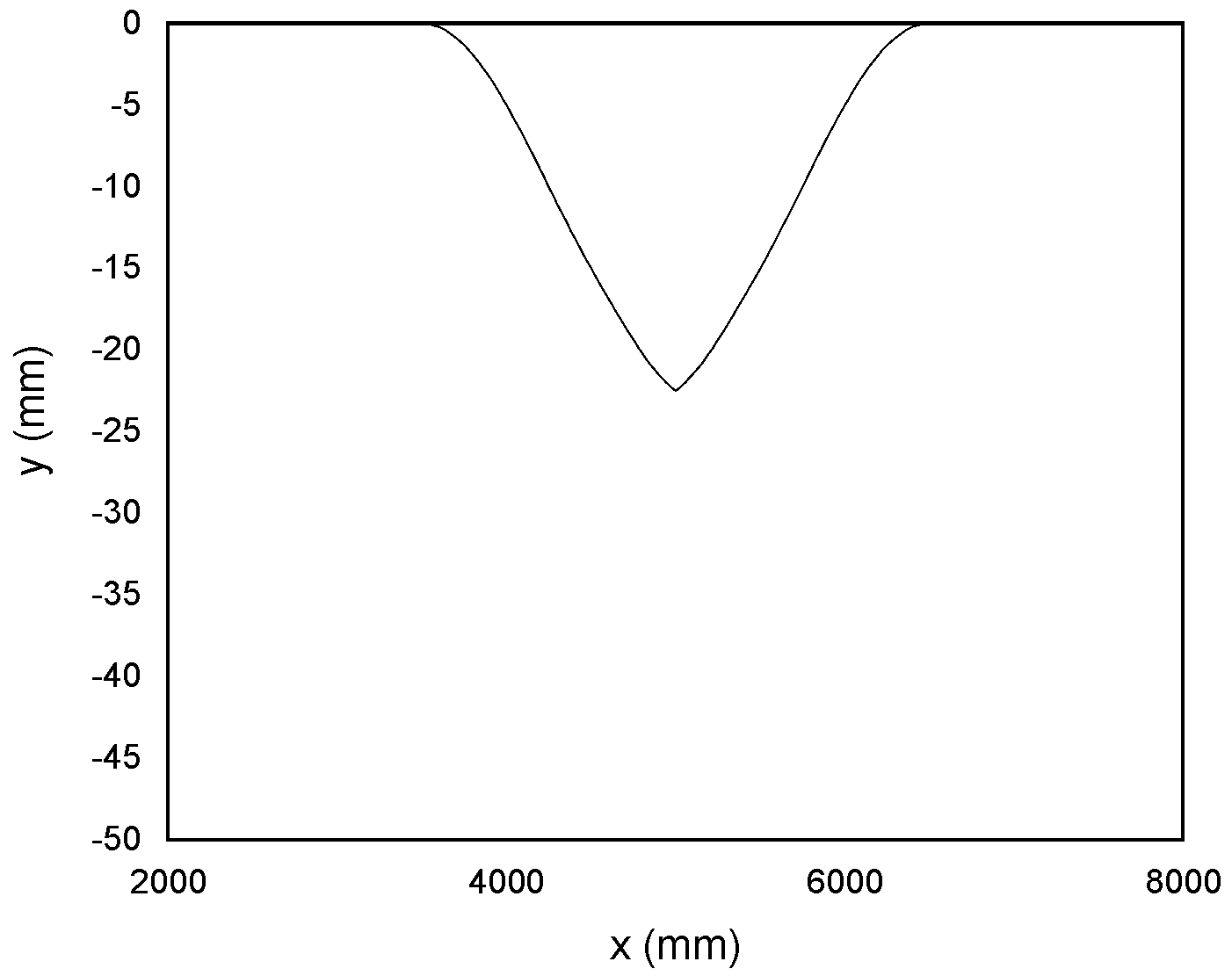
Table 2 shows the 1650 simulations run to simulate data. Examples of ABA are shown in Figure 1. The speed and weight of the rolling stock are 20 km/h and 40 tons respectively. Figure 1a presents ABA when the rail is free from defect, and Figure 1b presents ABA when the rail has the 2.5 mm dipped joint and 20 mm short settlement, as shown in Figure 2. These two figures show that the ABAs from the defect-free rail and the rail with defects are significantly different and easy to categorize. However, when the sizes of combined defects vary and the defects are combined, it will be more complicated to categorize the type and size of defect; machine learning plays an important role for this purpose. From Figure 1b, the ABA has peak and bottom values, which will be used as simplified features. Figure 1 presents only one ABA from a wheel. From the simulation, ABAs from two wheels are extracted and used as features.
The ABA is used in two ways as mentioned: simplified data and raw data. Simplified data are used to develop the DNN model, and raw data are used to develop the CNN and RNN models. For simplified data, 14 features are extracted from the simulations, which are the weight and speed of a rolling stock, three peak ABA from two wheels, and three bottom ABA from two wheels. In case of simplified data, the ABA is the result from simulations, but the weight and speed of a rolling stock are extracted before the simulation. This procedure is done under the assumption that the weight and speed are known from on-board sensors. The reason for using simplified data for the DNN model is that it is more suitable than using raw data. The authors have tried feeding the raw data into the DNN model where the number of input nodes is equal to the number of values. However, the performance is not satisfying. For raw data, ABAs from two wheels are fed into the models without processing and other features.
To process simplified data and arrange raw data, Visual Basic for Applications (VBA) is employed. Fourteen features are extracted from simulations’ reports and combined to create the dataset alongside raw data from each simulation. In this study, the total number of simulations is 1650, so the number of samples is the same. Each sample is labeled in accordance with the classes of each model. For defect severity classification, the labels are depending on the size of the defect, as shown in Table 3.

3.2. AI Model Development

DNN, CNN, and RNN are employed to develop machine learning models for detecting and evaluating the severity of combined defects. For dipped joint and settlement detection, this study proposes two approaches. The first approach is using a single model to detect both dipped joint and settlement. The second approach is using two independent models to detect dipped joint and settlement separately. This is to investigate whether a model has better performance for a more specific task. Therefore, the first approach will categorize four classes of the sample, namely, class 0: defect-free, class 1: dipped joint, class 2: settlement, and class 3: dipped joint and settlement. For the second approach, two models are used to detect dipped joint and settlement separately so the classes are binary, defect, and no defect.
For defect severity classification, samples are labeled as shown in Table 3. Models for classifying the severity of dipped joint and settlement are developed independently. It is noted that the second approach applies two models to detect each defect separately so the labels shown in Table 3 are dependent on the models. That means that label 0 in the dipped joint severity classification model is different from label 0 in the settlement severity classification model. For defect severity regression, the models are different because they are regression models in which the labels are real numbers. As defect severity classification, two models are developed for dipped joint and settlement severity evaluation.
The workflow of the machine learning models for detecting and evaluating combined defects is shown in Figure 3.
The features used to develop the DNN model consist of 14 features, as mentioned in the previous section. For CNN and RNN, two sets of raw data from two wheels’ ABA are used as features. The total number of values is 6695 for each wheel.
All models are tuned by hyperparameter tuning to ensure that all models provide the best performance. The detail is presented in the following section. In the training, samples are split using the proportion of 70/30. The performance of developed models is evaluated using accuracy in the case of classification and mean absolute error (MAE) in the case of regression. The models with the highest accuracy and the lowest MAE will be selected for further application.

3.3. Hyperparameter Tuning

Some parameters of the models are not tuned during the training. Hyperparameter tuning is conducted to improve the performance of models and ensure that the models provide the best performance. In this study, a grid search is used to tune hyperparameters. The list of tuned hyperparameters of each model is shown in Table 4.

4. Results and Discussion

This section presents the results of model development and discusses them by separating them into two topics, combined defect detection and combined defect severity evaluation. For combined defect detection, two approaches are applied as mentioned in the previous section. The first approach is developing a model to detect dipped joint and settlement, and the second approach is developing two models to detect dipped joint and settlement separately. Two approaches are compared to test the hypothesis of whether two models perform better than a single model for detecting combined defects.
The combined defect severity evaluation is presented into two topics: severity classification and severity regression. The classification is used to classify the severity of combined defects into groups as shown in Table 3. The regression is used to predict the size of combined defects. The performance of models is evaluated using the accuracy or MAE depending on the models. Three deep learning techniques are used, which are DNN, CNN, and RNN. The detail is presented as follows.

4.1. Combined Defect Detection

4.1.1. One Model for Detecting Both Dipped Joint and Settlement

There are four classes in this case, namely, no defect, dipped joint, settlement, and dipped joint and settlement. The performance of each model is presented in Table 5.
From Table 5, the accuracy of the CNN model is the highest followed by DNN and RNN, respectively. Surprisingly, the accuracy of the CNN model is almost 1.00; however, the accuracy of the RNN model is the worst, although both models use raw data as features. The DNN model performs quite well, although it does not perform as well as the CNN model and uses simplified data as features. From this, it can be concluded that using raw data does not guarantee higher accuracy than using simplified data. The RNN model has the lowest accuracy, from which it can be assumed that the technique is not suitable for classification in this condition. This is because the RNN model will perform well when it deals with the time-series data and the sequence of the data is significant. In this situation, the sequence of data is not highly related to each other. Therefore, the RNN model performs worse than other models. Moreover, training the RNN model takes the longest time compared to the DNN and CNN model. From the results, the CNN model is the best model for detecting combined defects in this approach. The tuned hyperparameters of the CNN model are shown in Table 6.

4.1.2. Two Models for Detecting Dipped Joint and Settlement Separately

This approach is to test whether the model has better performance if there are fewer classes to predict. Models are developed to detect dipped joint and settlement separately. The performance of each model is presented in Table 7.
From Table 7, the accuracy of models is calculated by multiplying the accuracy of the best models on dipped joint and settlement detections. The CNN model also has the best accuracy of 0.99. The overall performance of models is accorded to the first approach in which the CNN model has the highest accuracy followed by the DNN and RNN models. However, it is worth noting that the RNN model performs better than the DNN model in settlement detection. Compared to the first approach, it can be seen that the performance of models is improved when the number of classes is lower. However, the CNN model’s accuracy does not change. This might because the accuracy of the CNN model is high and there is no room for improvement. Although the performance of models can be improved by reducing the number of classes, the model developed in the first approach is good enough to detect combined defects. The CNN models from the two approaches perform the best and have the same accuracy of 0.99. The tuned hyperparameters of the CNN models are shown in Table 8.

4.2. Combined Defect Severity Evaluation

This section presents the results from model development to evaluate the combined defect severity after they are detected. To evaluate the severity, this study presents models to classify the severity and estimate the size of defects. In this part, dipped joint and settlement are considered separately, because the authors tried developing models to consider them together and found that the accuracy is not satisfied due to a too high number of classes to predict. Therefore, considering them separately is the better option.

4.2.1. Severity Classification

There are three classes to classify the severity of dipped joint and settlement, which are shown in Table 3. The accuracy of the classification of each model is presented in Table 9, and the confusion matrix of each model is presented as Table 10 and Table 11, respectively.
From Table 9, the CNN model is the best model for classifying the severity of dipped joint with an accuracy of 0.84, while the accuracy of the DNN and RNN models is not satisfied. The RNN model still performs worst for classifying the dipped severity. However, it is surprising that the RNN model has the highest accuracy in classifying the settlement severity with an accuracy of 0.99. This finding is conformed to the settlement detection model that the RNN model tends to perform well when dealing with the settlement. Therefore, the total accuracy of classifying combined defect severity is calculated from the accuracy of the CNN model on classifying the dipped joint severity and the accuracy of the RNN model on classifying the settlement severity, which equals 0.83. The tuned hyperparameters of each model are shown in Table 12.

4.2.2. Severity Regression

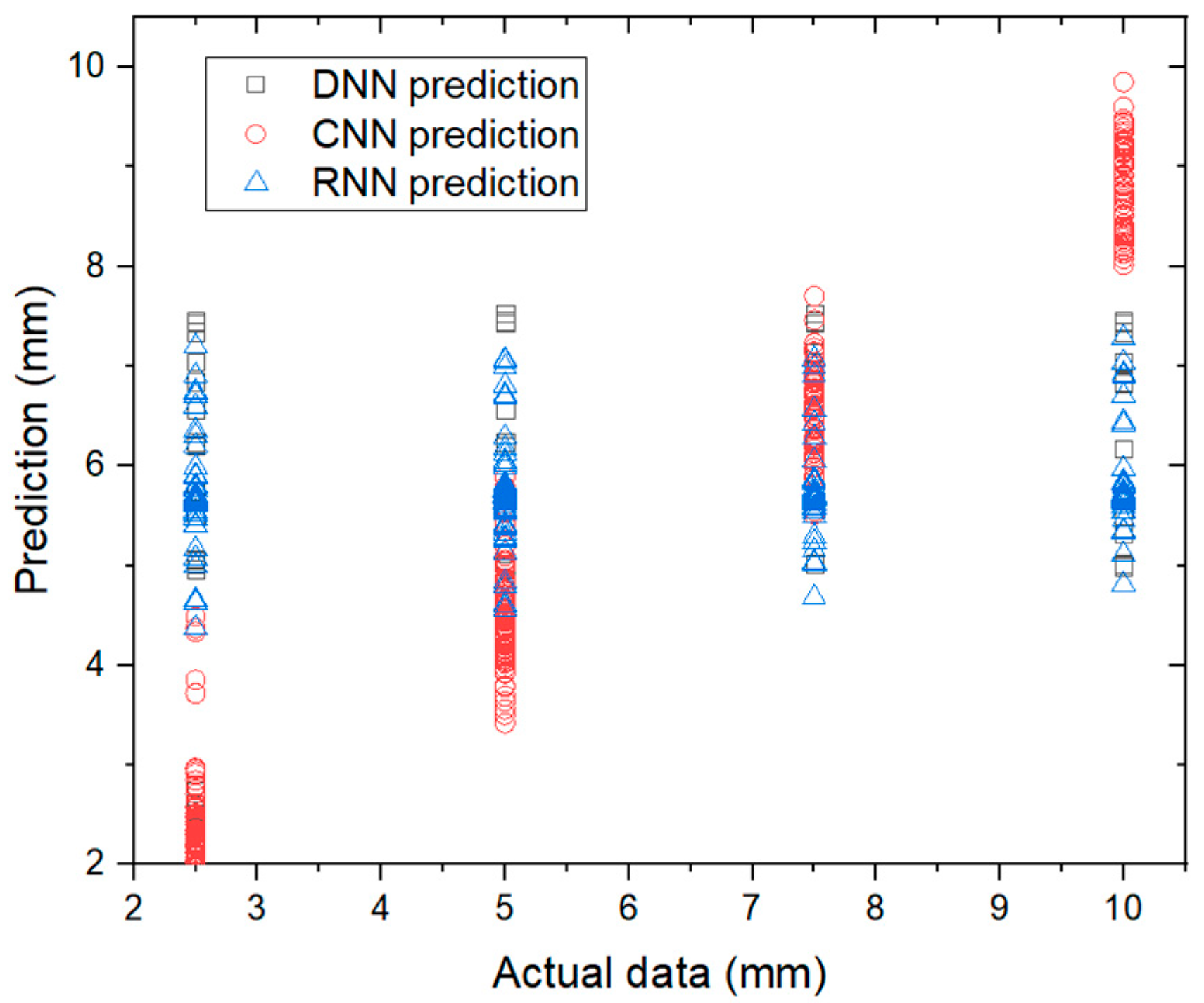
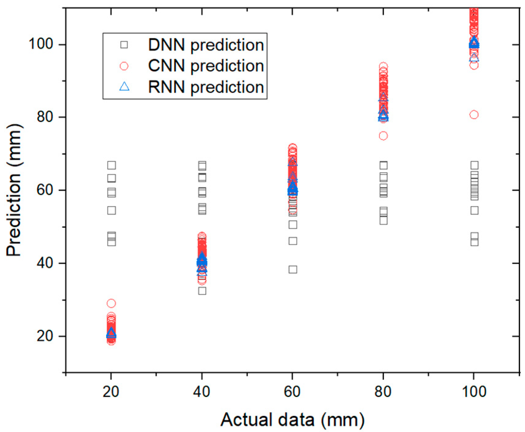
Models developed in this section are different from others because they are regression models. The output layer does not predict the class of data but the continuous value. As mentioned, the performance of each model is evaluated using MAE, which is straightforward to interpret compared to other indicators. The size of the defect is not labeled as groups, but it is directly used as a label. The performance of the severity regression or estimation is shown in Table 13. The plots between actual data and prediction are shown in Figure 4 and Figure 5 for dipped joint and settlement, respectively.
From Table 13 and Figure 4 and Figure 5, the CNN model is the best model for estimating the size of the dipped joint with the MAE of 1.25 mm, while the MAEs of the DNN and RNN models are lower, but the difference is not relatively high compared to the maximum size of 10 mm. The RNN model has the highest MAE. From the previous models, it can be concluded that the RNN model is not suitable for detecting and evaluating the dipped joint, which can be seen from the lowest performance in every aspect. Again, the RNN model has the lowest MAE on estimating the size of settlement, which equals 1.58 mm. Compared to the maximum size of settlement used in this study (100 mm), the RNN model can estimate the size of settlement with very low error. This emphasizes the performance of the RNN model on detecting and evaluating the settlement. It can be concluded that the CNN model is the best model for estimating the dipped joint size, and the RNN model is the best model for estimating the settlement size, which conformed to the model performance on the severity classification. The tuned hyperparameters of each model are shown in Table 14.

5. Conclusions

This study is the first to apply deep learning techniques to detect and evaluate the severity of combined defects in the railway infrastructure. Dipped joint and settlement are used as the case study of combined defects. The numerical data are simulated using D-Track, which is a verified simulation for studying the dynamic behavior of wheel and rail. Various parameters are used to create the diversity of data. There are 1650 simulations that are run. The output from the simulations that are used as features to develop the machine learning models is ABA from two wheels. ABA is used in two ways: simplified data and raw data. The DNN model uses the simplified data that consists of 14 features, while the CNN and RNN models use raw data. The data are split with the proportion of 70/30 to be data and testing data.
The models for detecting combined defects are developed using two approaches: a single model and two models for detecting combined defects. The study shows that using a single model is good enough to detect combined defects when the best model is the CNN model with an accuracy of 0.99. To evaluate the severity, models are developed to classify the severity and estimate the size of defects. It is found that the CNN models have the best performance in classifying and estimating the dipped joint with the accuracy and MAE of 0.84 and 1.25 mm respectively. However, the RNN models perform better in detecting and estimating the settlement with the accuracy and MAE of 0.99 and 1.58 mm, respectively.
To improve this unprecedented study, site data can emphasize the reliability of the finding in the study. The main difference between the simulated data and site data is that there are noises in site data. Other types of defects are also able to improve the capability of the model by increasing the variety of data. Other information is worth trying as features for model development to support other sensors and measurements.

Author Contributions

Conceptualization, S.K. and J.S.; methodology, J.S.; software, S.K.; validation, S.K. and J.S.; formal analysis, J.S.; investigation, J.S.; resources, S.K.; data curation, J.S.; writing—original draft preparation, J.S.; writing—review and editing, S.K.; visualization, J.S.; supervision, S.K.; project administration, S.K.; funding acquisition, S.K. All authors have read and agreed to the published version of the manuscript.

Funding

This research was funded by the European Commission, grant number 691135.

Institutional Review Board Statement

Not applicable.

Informed Consent Statement

Not applicable.

Data Availability Statement

The data presented in this study are available on request from the corresponding author. The data are not publicly available due to the confidentiality.

Acknowledgments

The authors also wish to thank the European Commission for the financial sponsorship of the H2020-RISE Project no.691135 “RISEN: Rail Infrastructure Systems Engineering Network”, which enables a global research network that addresses the grand challenge of railway infrastructure resilience and advanced sensing in extreme environments (www.risen2rail.eu, accessed on 21 January 2021) [44].

Conflicts of Interest

The authors declare no conflict of interest.

References

  1. Network Rail. Visual Track Inspection; Network Rail: London, UK, 2019. [Google Scholar]
  2. Network Rail. Ultrasonic Rail Inspection; Network Rail: London, UK, 2019. [Google Scholar]
  3. Bray, D.E. Historical review of technology development in NDE. In Proceedings of the 15th World Conference on NDT, Roma, Italy, 15–21 October 2000. [Google Scholar]
  4. Zhang, J.; Ma, H.; Yan, W.; Li, Z. Defect detection and location in switch rails by acoustic emission and Lamb wave analysis: A feasibility study. Appl. Acoust. 2016, 105, 67–74. [Google Scholar] [CrossRef]
  5. Zhang, X.; Feng, N.; Wang, Y.; Shen, Y. Acoustic emission detection of rail defect based on wavelet transform and Shannon entropy. J. Sound Vib. 2015, 339, 419–432. [Google Scholar] [CrossRef]
  6. Bruzelius, K.; Mba, D. An initial investigation on the potential applicability of Acoustic Emission to rail track fault detection. NDT E Int. 2004, 37, 507–516. [Google Scholar] [CrossRef] [Green Version]
  7. Rockstroh, B.; Kappes, W.; Walte, F.; Kröning, M.; Bessert, S.; Schäfer, W. Ultrasonic and eddy-current inspection of rail wheels and wheel set axles. In Proceedings of the 17th World Conference on Nondestructive Testing, Shanghai, China, 25–28 October 2008. [Google Scholar]
  8. Amerapex. Benefits of Non-Destructive Testing. 2020. Available online: https://amerapex.com/2014/12/benefits-non-destructive-testing/#:~:text=NDT%20is%20particularly%20effective%20because,those%20intended%20for%20future%20use (accessed on 20 January 2021).
  9. Wei, X.; Yang, Z.; Liu, Y.; Wei, D.; Jia, L.; Li, Y. Railway track fastener defect detection based on image processing and deep learning techniques: A comparative study. Eng. Appl. Artif. Intell. 2019, 80, 66–81. [Google Scholar] [CrossRef]
  10. ScienceDaily. Artificial Intelligence. 2020. Available online: https://www.sciencedaily.com/terms/artificial_intelligence.htm (accessed on 20 January 2021).
  11. Kumar, S. Advantages and Disadvantages of Artificial Intelligence. 2019. Available online: https://towardsdatascience.com/advantages-and-disadvantages-of-artificial-intelligence-182a5ef6588c (accessed on 20 January 2021).
  12. Huang, K.; Wu, J.; Yang, X.; Gao, Z.; Liu, F.; Zhu, Y. Discrete train speed profile optimization for urban rail transit: A data-driven model and integrated algorithms based on machine learning. J. Adv. Transp. 2019, 2019. [Google Scholar] [CrossRef]
  13. Alawad, H.; Kaewunruen, S.; An, M.J.I.A. Learning from accidents: Machine learning for safety at railway stations. IEEE Access 2019, 8, 633–648. [Google Scholar] [CrossRef]
  14. Sysyn, M.; Gerber, U.; Nabochenko, O.; Gruen, D.; Kluge, F. Prediction of rail contact fatigue on crossings using image processing and machine learning methods. Urban Rail Transit 2019, 5, 123–132. [Google Scholar] [CrossRef] [Green Version]
  15. Núñez, A.; Hendriks, J.; Li, Z.; De Schutter, B.; Dollevoet, R. Facilitating maintenance decisions on the Dutch railways using big data: The ABA case study. In Proceedings of the 2014 IEEE International Conference on Big Data (Big Data), Washington, DC, USA, 27–30 October 2014. [Google Scholar]
  16. Li, Z.; Molodova, M.; Núñez, A.; Dollevoet, R. Improvements in Axle Box Acceleration Measurements for the Detection of Light Squats in Railway Infrastructure. IEEE Trans. Ind. Electron. 2015, 62, 4385–4397. [Google Scholar] [CrossRef]
  17. Molodova, M. Detection of early squats by axle box acceleration. Engineering 2013. [Google Scholar] [CrossRef]
  18. Molodova, M.; Li, Z.; Núñez, A.; Dollevoet, R. Validation of a finite element model for axle box acceleration at squats in the high frequency range. Comput. Struct. 2014, 141, 84–93. [Google Scholar] [CrossRef]
  19. Song, Y.; Liang, L.; Du, Y.; Sun, B. Railway Polygonized Wheel Detection Based on Numerical Time-Frequency Analysis of Axle-Box Acceleration. Appl. Sci. 2020, 10, 1613. [Google Scholar] [CrossRef] [Green Version]
  20. Wei, Z.; Núñez, A.; Li, Z.; Dollevoet, R. Evaluating Degradation at Railway Crossings Using Axle Box Acceleration Measurements. Sensors 2017, 17, 2236. [Google Scholar]
  21. Molodova, M.; Oregui, M.; Núñez, A.; Li, Z.; Dollevoet, R. Health condition monitoring of insulated joints based on axle box acceleration measurements. Eng. Struct. 2016, 123, 225–235. [Google Scholar] [CrossRef] [Green Version]
  22. Oregui, M.; Li, S.; Núñez, A.; Li, Z.; Carroll, R.; Dollevoet, R. Monitoring bolt tightness of rail joints using axle box acceleration measurements. Struct. Contr. Health Monit. 2017, 24, e1848. [Google Scholar] [CrossRef] [Green Version]
  23. Real Herráiz, J.I.; Montalbán Domingo, M.L.; Real, T.; Puig, V. Development of a system to obtain vertical track geometry measuring axle-box accelerations from in-service trains. J. Vibroengineering 2012, 14, 813–826. [Google Scholar]
  24. Deutschl, E.; Gasser, C.; Niel, A.; Werschonig, J. Defect detection on rail surfaces by a vision based system. In Proceedings of the IEEE Intelligent Vehicles Symposium, Parma, Italy, 14–17 June 2004. [Google Scholar]
  25. Mandriota, C.; Nitti, M.; Ancona, N.; Stella, E.; Distante, A. Filter-based feature selection for rail defect detection. Mach. Vis. Appl. 2004, 15, 179–185. [Google Scholar] [CrossRef]
  26. Jie, L.; Siwei, L.; Qingyong, L.; Hanqing, Z.; Shengwei, R. Real-time rail head surface defect detection: A geometrical approach. In Proceedings of the 2009 IEEE International Symposium on Industrial Electronics, Seoul, Korea, 5–8 July 2009. [Google Scholar]
  27. Feng, H.; Jiang, Z.; Xie, F.; Yang, P.; Shi, J.; Chen, L. Automatic fastener classification and defect detection in vision-based railway inspection systems. IEEE Trans. Instrum. Meas. 2013, 63, 877–888. [Google Scholar] [CrossRef]
  28. Tastimur, C.; Yetis, H.; Karaköse, M.; Akin, E. Rail defect detection and classification with real time image processing technique. Int. J. Comput. Sci. Softw. Eng. 2016, 5, 283. [Google Scholar]
  29. Xiong, Z.; Li, Q.; Mao, Q.; Zou, Q. A 3D laser profiling system for rail surface defect detection. Sensors 2017, 17, 1791. [Google Scholar] [CrossRef] [Green Version]
  30. Kang, G.; Gao, S.; Yu, L.; Zhang, D. Deep architecture for high-speed railway insulator surface defect detection: Denoising autoencoder with multitask learning. IEEE Trans. Instrum. Meas. 2018, 68, 2679–2690. [Google Scholar] [CrossRef]
  31. Krummenacher, G.; Ong, C.S.; Koller, S.; Kobayashi, S.; Buhmann, J.M. Wheel Defect Detection With Machine Learning. IEEE Trans. Intell. Transp. Syst. 2018, 19, 1176–1187. [Google Scholar] [CrossRef]
  32. Yu, H.; Li, Q.; Tan, Y.; Gan, J.; Wang, J.; Geng, Y.A.; Jia, L. A coarse-to-fine model for rail surface defect detection. IEEE Trans. Instrum. Meas. 2018, 68, 656–666. [Google Scholar] [CrossRef]
  33. Zhang, Z.; Zhou, K.; Liu, X. Broken Rail Prediction With Machine Learning-Based Approach. In ASME/IEEE Joint Rail Conference 2020; American Society of Mechanical Engineers: New York, NY, USA, 2020. [Google Scholar]
  34. Cai, Z. Modelling of Rail Track Dynamics and Wheel/Rail Interaction; Queen’s University: Kingston, ON, Canada, 1994. [Google Scholar]
  35. Steffens, D.M. Identification and Development of a Model of Railway Track Dynamic Behaviour. Master’s Thesis, Queensland University of Technology, Brisbane City, Australia, 2005. [Google Scholar]
  36. Leong, J. Development of a Limit State Design Methodology for Railway Track. Master’s Thesis, Queensland University of Technology, Brisbane City, Australia, 2007. [Google Scholar]
  37. Kaewunruen, S.; Osman, M.H.B.; Rungskunroch, P. The Total Track Inspection. Front. Built Environ. 2019, 4, 84. [Google Scholar] [CrossRef] [Green Version]
  38. Kaewunruen, S. Monitoring of rail corrugation growth on sharp curves for track maintenance prioritization. Int. J. Acoustic. Vib. 2018, 23, 35–43. [Google Scholar] [CrossRef]
  39. Kaewunruen, S.; Chiengson, C. Railway track inspection and maintenance priorities due to dynamic coupling effects of dipped rails and differential track settlements. Eng. Fail. Anal. 2018, 193, 157–171. [Google Scholar] [CrossRef]
  40. Bin Osman, M.H.; Kaewunruen, S.; Jack, A. Optimisation of schedules for the inspection of railway tracks. Proc. Inst. Mech. Eng. Part F J. Rail Rapid Transit 2018, 232, 1577–1587. [Google Scholar] [CrossRef]
  41. Remennikov, A.M.; Kaewunruen, S. A review of loading conditions for railway track structures due to train and track vertical interaction. Struct. Cont. Health Mon. 2008, 15, 207–234. [Google Scholar] [CrossRef]
  42. Alawad, H.; Kaewunruen, S. 5G Intelligence Underpinning Railway Safety in the COVID-19 Era. Front. Built Environ. 2021, 7, 639753. [Google Scholar] [CrossRef]
  43. Kaewunruen, S.; Sresakoolchai, J.; Ma, W.; Phil-Ebosie, O. Digital Twin Aided Vulnerability Assessment and Risk-Based Maintenance Planning of Bridge Infrastructures Exposed to Extreme Conditions. Sustainability 2021, 13, 2051. [Google Scholar] [CrossRef]
  44. Kaewunruen, S.; Sussman, J.M.; Matsumoto, A. Grand Challenges in Transportation and Transit Systems. Front. Built Environ. 2016, 2, 4. [Google Scholar] [CrossRef] [Green Version]
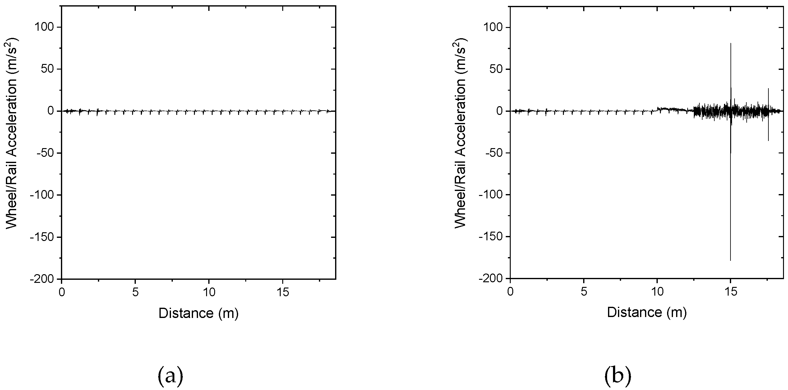
Figure 1. Examples of output from D-track simulation: (a) ABA from defect-free rail; (b) ABA from the rail with a dipped joint and settlement.
Vibration 04 00022 g001
Figure 2. Examples of profile for running the simulation (dipped joint of 2.5 mm and short settlement of 20 mm).
Vibration 04 00022 g002
Figure 3. Workflow of the machine learning models.
Vibration 04 00022 g003
Figure 4. Actual data and prediction of dipped joint severity regression.
Vibration 04 00022 g004
Figure 5. Actual data and prediction of settlement severity regression.
Vibration 04 00022 g005
Table 1. Summarized list of studies using machine learning to detect railway defects.
YearAuthorsDefectsTechniquesInputPrediction
2004Deutschl et al. [24]Surface defectVision-based systemImageDefect-free, defect, and suspicious
2004Mandriota et al. [25]CorrugationFilter-based feature selectionImageDefect and no-defect
2009Jie et al. [26]Rail head surface defectVision-based systemImageDefect and no-defect
2013Feng et al. [27]Fastener defectVision-based systemImageWorn and missing fasteners
2016Tastimur et al. [28]Rail surface defectAdaBoostImageHeadcheck, undulation, scour, and fracture defects
2017Xiong et al. [29]Rail surface defect3D laser profiling systemSurface profileAbrasion, corrugation, scratch, corrosion, and peeling
2018Kang et al. [30]Insulator surface defectCNNImageDefect and no-defect
2018Krummenacher et al. [31]Flat spot, shelling, and non-roundnessSupport vector machine and DNNForce and imageDefect and no-defect
2018Yu et al. [32]Rail surface defectCoarse-to-fine modelImageDefect and no-defect
2019Wei et al. [9]Fastener defectImage processingImageComplete, broken, and missing fasteners
2020Zhang et al. [33]Broken railExtreme gradient boostingTrack characteristics, traffic-related information, maintenance records, and historical defect recordsDefect and no-defect
Table 2. A summary of varied parameters in D-Track.
ParametersValue
Sizes of dipped joint0–10 mm (the length of the dipped joint is 1000 mm.)
Sizes of settlement0–100 mm (the lengths of the settlement are 3000 and 10,000 mm for short and long settlement, respectively)
Speeds of vehicle20–200 km/h
Weights of vehicle40–80 tons
Rail typeAS60
GaugeStandard gauge
Pad typeHDPE
Sleeper typePrestressed
Sleeper spacing600–750 mm
Track bed stiffness50.1 MN/m
Track bed damping159 kNs/m
Primary suspension stiffness1.22 MN/n
Primary suspension damping4 kNs/m
Wheel radius460 mm
Hertzian contact coefficient7.25 × 1010 N/M3/2
Table 3. A summary of the label for each model.
PurposeType of LabelLabelMeaning
Dipped joint severity classificationInteger0
1
2
2.5 mm or smaller
2.5–5.0 mm
Bigger than 5.0 mm
Settlement severity classificationInteger0
1
2
20 mm or smaller
20–60 mm
Bigger than 60 mm
Table 4. List of tuned hyperparameters.
ModelTuned Hyperparameter
DNN
  • The number of hidden layers
  • The number of hidden nodes
  • Activation function
  • Batch size
  • Learning rate
  • Momentum
  • Optimizer
  • Dropout
CNN
  • The number of convolutional layers
  • Filter
  • Kernel
  • The number of max pooling layers
  • Pool size
  • The number of hidden layers
  • The number of hidden nodes
  • Activation function
  • Batch size
  • Learning rate
  • Momentum
  • Optimizer
  • Dropout
RNN
  • The number of LSTM cells
  • The number of hidden layer
  • The number of hidden node
  • Activation function
  • Batch size
  • Learning rate
  • Momentum
  • Optimizer
  • Dropout
Table 5. Performance of each model for detecting combined defects.
ModelAccuracy
DNN0.86
CNN0.99
RNN0.79
Table 6. List of tuned hyperparameters for detecting combined detects in the first approach.
ModelTuned HyperparameterValue
CNNThe number of convolutional layers2
Filter80 (conv1) and 64 (conv2)
Kernel5
The number of max pooling layers2
Pool size3
The number of hidden layers2
The number of hidden nodes100
Activation functionReLu (except dense3 which uses Softmax)
Batch size64
Learning rate0.001
Momentum0.9
OptimizerAdam
DropoutN/A
Table 7. Performance of each model for detecting dipped joint and settlement.
ModelAccuracy
Dipped joint detection
DNN0.94
CNN1.00
RNN0.86
Settlement detection
DNN0.92
CNN0.99
RNN0.94
Total accuracy0.99
Table 8. List of tuned hyperparameters for detecting combined detects in the second approach.
ModelTuned HyperparameterValue
CNN for detecting dipped jointThe number of convolutional layers2
Filter64 (conv1) and 32 (conv2)
Kernel7
The number of max pooling layers2
Pool size2
The number of hidden layers2
The number of hidden nodes100
Activation functionReLu (except dense3, which uses Softmax)
Batch size64
Learning rate0.001
Momentum0.9
OptimizerAdam
Dropout0.25 (before maxpooling2)
CNN for detecting settlementThe number of convolutional layers2
Filter80 (conv1) and 64 (conv2)
Kernel6
The number of max pooling layers2
Pool size4
The number of hidden layers2
The number of hidden nodes100
Activation functionReLu (except dense3 which uses Softmax)
Batch size64
Learning rate0.001
Momentum0.9
OptimizerAdam
DropoutN/A
Table 9. Performance of each model for detecting dipped joint and settlement.
ModelAccuracy
Dipped joint severity classification
DNN0.61
CNN0.84
RNN0.51
Settlement severity classification
DNN0.51
CNN0.95
RNN0.99
Total Accuracy0.83
Table 10. Confusion matrix of dipped joint severity classification from the convolutional neural network (CNN) model.
Predicted Class 0Predicted Class 1Predicted Class 2
Actual Class 075816
Actual Class 156924
Actual Class 219189
Table 11. Confusion matrix of settlement severity classification from the recurrent neural network (RNN) model.
Predicted Class 0Predicted Class 1Predicted Class 2
Actual Class 09410
Actual Class 111710
Actual Class 201182
Table 12. List of tuned hyperparameters for classifying the combined detect severity.
ModelTuned HyperparameterValue
CNN for classifying dipped joint severityThe number of convolutional layers2
Filter32
Kernel9
The number of max pooling layers2
Pool size3 (maxpoo1ing1) and 6 (maxpooling2)
The number of hidden layers2
The number of hidden nodes80
Activation functionReLu (except dense3, which uses Softmax)
Batch size8
Learning rate0.001
Momentum0.9
OptimizerAdam
DropoutN/A
RNN for classifying settlement severityThe number of LSTM cells200
The number of hidden layer2
The number of hidden node100
Activation functionReLu (except dense3, which uses Softmax)
Batch size64
Learning rate0.001
Momentum0.9
OptimizerAdam
DropoutN/A
Table 13. Performance of each model for estimating the size of dipped joint and settlement.
ModelMAE (mm)
Dipped joint severity regression
DNN2.01
CNN1.25
RNN2.54
Settlement severity regression
DNN21.14
CNN3.13
RNN1.58
Table 14. List of tuned hyperparameters for estimating the combined detect severity.
ModelTuned HyperparameterValue
CNN for estimating dipped joint severityThe number of convolutional layers2
Filter32 (conv1) and 64 (conv2)
Kernel5 (conv1) and 4 (conv2)
The number of max pooling layers2
Pool size3 (maxpoo1ing1) and 2 (maxpooling2)
The number of hidden layers2
The number of hidden nodes100 (dense1) and 50 (dense2)
Activation functionReLu (except dense3, which uses Linear)
Batch size16
Learning rate0.001
Momentum0.9
OptimizerAdam
DropoutN/A
RNN for estimating settlement severityThe number of LSTM cells200
The number of hidden layer2
The number of hidden node200
Activation functionReLu (except dense3, which uses Linear)
Batch size8
Learning rate0.001
Momentum0.9
OptimizerAdam
DropoutN/A
Publisher’s Note: MDPI stays neutral with regard to jurisdictional claims in published maps and institutional affiliations.