Friction-Induced Vibration in a Bi-Stable Compliant Mechanism

Abstract

This paper investigates friction-induced self-excited vibration in a bi-stable compliant mechanism. A single-degree-of-freedom oscillator, hanged vertically, vibrates on a belt moving horizontally with a constant velocity. The oscillator is excited through the frictional input provided by the belt. The friction coefficient is defined as an exponentially decaying function of the sliding velocity. Due to the specific configuration of spring and damper, the normal contact force is variable. Therefore, the friction force is a function of the system states, namely, slider velocity and position. Employing eigenvalue analysis gives an overview of the local stability of the linearized system in the vicinity of each equilibrium point. It is shown that the normal force, spring pre-compression and belt velocity are bifurcation parameters. Since the system is highly nonlinear, a local analysis does not provide enough information about the steady-state response. Therefore, the oscillating system is studied numerically to attain a global qualitative picture of the steady-state response. The possibility of the mass-belt detachment and overshoot are studied. It is shown that one equilibrium point is always dominant. In addition, three main questions, i.e., possible mass-belt separation, location of stick-slip transition and overshoot are answered. It is proven that the occurrence of overshoot is impossible.

1. Introduction

Compliant mechanisms are widely employed in various applications due to their potential advantages over conventional mechanisms, from a designing and manufacturing point of view [1]. Despite the extensive research carried out into compliant mechanisms, the self-excited vibration of such mechanisms has not been studied yet. Friction-induced vibration is considered as one of the main self-excited oscillations in various engineering applications.

Phenomena associated with friction-induced instability appear in a wide range of engineering applications known as the main reason for undesired noise and excessive wear [2,3,4,5,6,7,8,9,10,11,12]. Three main destabilizing mechanisms are known as the stem of friction-induced instability, namely, the Stribeck effect, Sprag-slip and mode-coupling [13]. The Stribeck effect occurs due to the negative damping induced by the velocity-decaying friction coefficient [3]. The Sprag-slip mechanism happens because of self-locking of the slider [13]. It is interesting to note that in current research, the Stribeck effect and Sprag-slip coexist while the occurrence of the latter depends on the former. To the best of our knowledge, such behavior is not observed in the previous literature. Olejnik and Awrejcewicz conducted an in-depth study on the accuracy of numerical solutions to solve friction-induced instability of a system with Filippov-type equations of motion [7]. Also, they investigated effects of two different coefficients of friction on a two DOF (Degree-of-Freedom) mass-on-belt model [2].

A discrete mass-on-belt model in spite of its simplicity can present the nonlinear nature of friction-induced vibration that occurs in many mechanical systems [3,4]. Such a model is useful to simulate stick-slip instability and capture fundamental nonlinear behavior for different applications such as wiper blade [14], asperities or contact patches in a contact interface of two sliding surfaces [15] and even drill strings [16,17]. In the majority of articles, normal contact load is considered constant which is an acceptable assumption unless the system undergoes large deflection, then the normal contact force is variable [7,18,19]. In addition, models with one degree of freedom usually possess a single equilibrium point and may undergo Hopf-bifurcation based on the definition of friction coefficient. However, the existence of more than one equilibrium point in a mass-on-belt system under external harmonic excitation with constant coefficient of friction was studied in Reference [18]. In Reference [18] the frictional system is stable in the absence of harmonic excitation, in other words, the aforementioned mechanisms of friction-induced instability are not involved in the problem. Li et. al. then studied friction-induced instability in an asymmetrical archetypal self-excited oscillator by introducing the Stribeck effect, where the damping force does not have a vertical component [19]. This model does not properly represent the viscoelastic behavior in the system. In case of a Kelvin–Voigt viscoelastic model, spring and damper have a parallel configuration [20].

Compliant mechanisms are defined as flexible structures without joints. Howell thoroughly studied compliant mechanisms [1] and introduced a pseudo-rigid-body model to simplify the design of the mechanisms. In a pseudo-rigid-body model, a flexible link is replaced by a proper combination of a rigid segment and translational or torsional springs. Although the flexible links in a compliant mechanism present nonlinear force-displacement relations, a linear spring can provide a reasonable approximation by means of a pseudo-rigid-body model [1,21]. An important category of such a mechanism is called a bi-stable compliant mechanism which possessed two distinct stable equilibrium positions in the absence of any external force input and has applications in valves and switches [1,21]. Research carried out on the bi-stable compliant mechanisms lack the study of self-sustained vibrations in such mechanisms, which is the subject of the present article.

In the current paper, we investigated the friction-induced vibration in a bi-stable compliant mechanism with large displacement and variable normal contact force. The study considered the effect of self-excited vibration on the static equilibrium points of the mechanism. The bi-stable compliant mechanism was modeled by its equivalent pseudo-rigid-body model. A parallel configuration of spring-damper represented viscoelastic behavior in the model. The system was excited by frictional force through a moving belt in contact with the oscillator. The friction coefficient was defined as a, well-known, exponentially decaying function of the relative velocity in contact interface. Such a definition of friction provided an equivalent negative damping, i.e., Stribeck effect, in the system which may have caused instability. Due to large deflection of the spring, the normal contact force and consequently friction force were functions of the state displacement and velocity vectors of the system. Considering bifurcation parameters that include belt velocity, applied normal force and spring pre-compression, it was shown that two bifurcation events occur. The belt velocity led to subcritical Hopf-bifurcation, where an unstable equilibrium point transformed to a stable one enclosed by an unstable limit cycle. While the two other parameters (applied normal force and spring pre-compression) caused pitchfork bifurcation, i.e., the system may have possessed either one or three equilibrium points. It was found that one equilibrium point was dominant during steady-state oscillation. In addition, Sprag-slip response can be observed in the proposed model when the oscillator experienced self-locking against the sliding surface.

2. Mechanical Model

The model consists of a mass sliding on a moving belt with constant velocity ($v_b$) and is supported by a spring and dashpot that rotate freely as shown in Figure 1. In addition, a constant applied normal load ($N$) is chosen large enough so as to prevent the mass from loss of contact with the belt. An exponential decaying function which accounts for the Stribeck effect is assumed to define the coefficient of friction,$\mu$. Moreover, the angle between the spring-dashpot and the direction of sliding is denoted $\theta$, the free length of spring is $a_0$ and the pre-compression length of spring in the vertical position ($\theta =90$)$h$. The condition $a_0>h$ is necessary so that the spring in the vertical position is compressed. It should be noted that the contact force varies as mass oscillates on the belt due to normal components of elastic and viscous forces. In this article, the right-side refers to the positive $x$ position of the mass, i.e., $x>0$, and the left-side implies negative $x$ position of the mass.

One may find the equation of motion in the following form [18,19]

$$m\ddot{x}+\left(F_d+F_k\right)\cos \left(\theta \right)=\mu \left(\mathrm{N}-\left(F_d+F_k\right)\sin \left(\theta \right)\right)\mathrm{sign}\left(v_b-\dot{x}\right),$$

(1)

where $F_d$ and $F_k$, the viscous and elastic force due to damper and spring, respectively, are defined as follows

$$F_k=k\left(a-a_0\right),F_d=c\dot{a}.$$

(2)

Pertinent geometric relations are

$$\cos (\theta )=\frac{x}{a},\sin (\theta )=\frac{h}{a},$$

(3)

where the length of the spring is $a=\sqrt{x^2+h^2}$ and its derivative with respect to time is $\dot{a}=\frac{x\dot{x}}{a}$. By substituting Equation (2) into Equation (1) and introducing dimensionless time $\tau =\omega t$, where $\omega =\sqrt{\frac{k}{m}}$, and dimensionless coordinate $z=\frac{x}{h}$, the equation of motion in dimensionless form is obtained.

$$\ddot{z}+\zeta \frac{z^2}{z^2+1}\dot{z}+(1-\frac{\alpha }{\sqrt{z^2+1}})z=\mu (n-(1-\frac{\alpha }{\sqrt{z^2+1}})-\zeta \frac{z}{z^2+1}\dot{z})\mathrm{sign}(V-\dot{z}),$$

(4)

where over dot denotes differentiation with respect to dimensionless time $\tau$. Damping ratio is $\xi =\frac{c}{m\omega }$, spring pre-compression ratio $\alpha =\frac{a_0}{h}$, dimensionless normal load $n=\frac{N}{kh}$ and dimensionless belt velocity $V=\frac{v_b}{\omega h}$. In addition, an exponential description for sliding coefficient of friction is defined as follows [3]

$$\mu ={\mu }_k+\left({\mu }_s-{\mu }_k\right)e^{-d\left|V-\dot{z}\right|}.$$

(5)

The tuning parameter $d=20$ defines the decaying slope of the friction coefficient at low relative velocity. Static friction coefficient, ${\mu }_s=0.6$, is the maximum value that occurs during stick phase and ${\mu }_k=0.3$ is the minimum friction coefficient at relatively high sliding velocities.

3. Linearized Stability

Defining state variables as $u_1=z$ and $u_2=\dot{z}$, it is convenient to rewrite Equation (4) in the state space form

$$\begin{array}{}{\dot{u}}_1=u_2\\ {\dot{u}}_2=-\zeta \frac{u_1{}^2}{u_1{}^2+1}{u}_2-\left(1-\frac{\alpha }{\sqrt{u_1{}^2+1}}\right)u_1+\mu \left(n-\left(1-\frac{\alpha }{\sqrt{u_1{}^2+1}}\right)-\zeta \frac{u_1}{u_1{}^2+1}{u}_2\right)\mathrm{sign}\left(V-u_2\right).\end{array}$$

(6)

Putting ${\dot{u}}_1={\dot{u}}_2=0$ into Equation (3) equilibrium points of the system are real roots of

$$-\left(1-\frac{\alpha }{\sqrt{u_1{}^2+1}}\right)u_1+{\mu }_0\left(n-\left(1-\frac{\alpha }{\sqrt{u_1{}^2+1}}\right)\right)=0,$$

(7)

where ${\mu }_0={\mu }_k+\left({\mu }_s-{\mu }_k\right)e^{-dV}$. For an applicable range of $\alpha$, $n$ and $\mu$, Equation (7) may possess either one or three roots (Figure 2). In the latter case, two roots are either stable or unstable spirals and a root located somewhere between them is a saddle. Due to geometric nonlinearity, the roots of Equation (7) is obtained numerically as shown in Figure 2. From Figure 2a, which demonstrates the variation of equilibrium point versus dimensionless velocity of the belt, it can be observed that the number of fixed points is independent of velocity, but their location may slightly change in the low range velocities. Figure 2b represents the effect of dimensionless normal load on the equilibrium points of the system. It is seen that the saddle and one spiral merge together as normal force is increased, meanwhile the position of the other spiral moves to the right, away from the origin. Finally, at $n=2.7$, the saddle and the left spiral points vanish. Figure 2c shows the equilibrium points as the spring pre-compression is changed. In the range $\alpha <2$ there is just one spiral point, for larger $\alpha$, one saddle (middle dashed line) and another spiral appear. The bifurcation observed in Figure 2b,c can be explained as the balance between the friction and elastic forces. In other words, as long as the friction force is dominant, i.e., regardless of $\alpha$ value, the system possesses just one equilibrium point. While, in the case that these forces are comparable, two other equilibrium points appear.

The local stability of the system is studied in the vicinity of spirals ($V-u_2>0$). For this purpose a Jacobian matrix, $J$ is found as

$$J=\left[\begin{array}{cc}0& 1\\ j_{21}& j_{22}\end{array}\right].$$

(8)

It is important to note that since the argument inside the signum function in the vicinity of the equilibrium point is greater than zero, i.e., $\mathrm{sign}\left(V-u_2\right)=1$, therefore, the equation of motion is a smooth function and its partial derivatives with respect to state variables ($u_1$ and $u_2$) can be calculated. The Jacobian matrix elements derived as follows:

$$\begin{array}{}{j}_{21}=-1-\frac{u_1^2\alpha }{{\left(1+u_1^2\right)}^{\frac{3}{2}}}+\frac{\alpha }{\sqrt{1+u_1^2}}+\frac{2u_1^3{u}_2}{{\left(1+u_1^2\right)}^2}\xi -\frac{2u_1{u}_2}{1+u_1^2}\xi +\mu \left(\frac{2u_1^2{u}_2}{{\left(1+u_1^2\right)}^2}\xi -\frac{u_1\alpha }{{\left(1+u_1^2\right)}^{\frac{3}{2}}}-\frac{u_2}{1+u_1^2}\xi \right),\\ j_{21}=-\frac{u_1^2}{1+u_1^2}\xi +d\left({\mu }_s-{\mu }_k\right)e^{-d\left(V-u_2\right)}\left(n-1+\frac{\alpha }{\sqrt{1+u_1^2}}-\frac{u_1{u}_2}{1+u_1^2}\xi \right)-\frac{u_1}{1+u_1^2}\mu \xi .\end{array}$$

(9)

Eigenvalue analysis of the Jacobian matrix at equilibrium points determines their local stability.

$$Det\left(J-\lambda I\right)={\lambda }^2-j_{22}\lambda -j_{21},$$

(10)

where $Det$ stands for the determinant of the argument, $\lambda$ is the eigenvalue at the corresponding equilibrium point and $I$ is the identity matrix. The real part of the eigenvalue determines the stability of the corresponding equilibrium point. Figure 3 illustrates the variation of the real parts of the eigenvalues versus belt velocity for three damping ratios. As the belt velocity increased, the positive real part of the eigenvalues started from all being positive and decreased until most crossed the zero value and entered the negative range. Only for the undamped system ($\zeta =0$) the real part of the eigenvalues merged at $Re\left[\lambda \right]=0$. Adding viscous damping to the system, made the spirals stable after a critical belt velocity was exceeded. It was interesting to note that the spiral located on the right side ($u_1>0$) became stable sooner than the one on the left. Therefore, three different stability conditions for spirals can occur: (1) two spiral sources at the relatively low range of the belt velocity, (2) a spiral source on the left along with a spiral sink on the right, and finally, (3) two spiral sinks for relatively high belt speed. The specific range of the belt velocity depends on the damping coefficient as depicted in Figure 3. The way the stability of the spirals affected steady-state response of the oscillator will be discussed later in this paper.

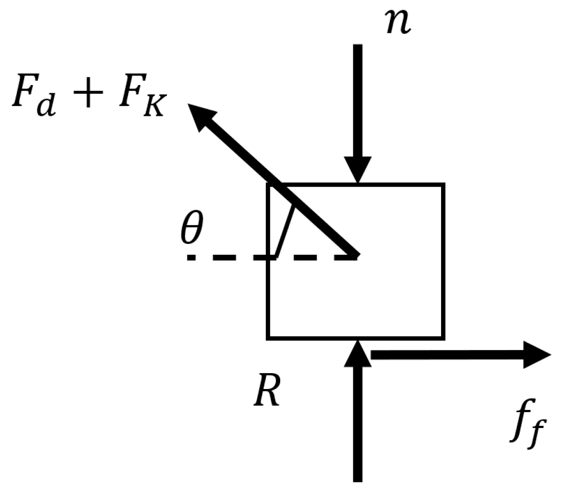
4. Mass-Belt Detachment

Assumption is mass does not lose contact with belt. As shown in free diagram, Figure 4, the normal contact force is $R$, and detachment happens if the contact force nullifies, i.e., $R=0$.

The normal contact load from the right-hand side of Equation (4), is

$$R=n-\zeta \frac{z}{z^2+1}\dot{z}-\left(1-\frac{\alpha }{\sqrt{z^2+1}}\right).$$

(11)

By letting $R=0$, one can define the condition of detachment as

$$n-1=\zeta \frac{z}{z^2+1}\dot{z}-\frac{\alpha }{\sqrt{z^2+1}}.$$

(12)

In the current paper the constant normal force was chosen to be greater than $n\ge 1$, therefore

$$\zeta \frac{z}{z^2+1}\dot{z}-\frac{\alpha }{\sqrt{z^2+1}}\ge 0.$$

(13)

For an undamped oscillator, $\zeta =0$, so

$$-\frac{\alpha }{\sqrt{z^2+1}}\ge 0,$$

(14)

which is not valid since the spring compression parameter is always positive ($\alpha \ge 1$).

For a damped system, one should study two different cases separately, for positive and negative displacement.

When the oscillator is moving on the right side, i.e., $z>0$, then

$$\dot{z}\ge \frac{\alpha }{\zeta }\frac{\sqrt{z^2+1}}{z}.$$

(15)

For $z<0$:

$$\dot{z}\le \frac{\alpha }{\zeta }\frac{\sqrt{z^2+1}}{z}.$$

(16)

In the paper, cases with $\alpha =3$, $n=1$, and $\zeta =0.01$ were studied, i.e., $\frac{\alpha }{\zeta }=300$. Due to spring pre-compression, detachment could happen for large horizontal displacement, so one can deduce

$$\frac{\sqrt{z^2+1}}{z}\approx 1\left(z>0\right)\mathrm{and}\frac{\sqrt{z^2+1}}{z}\approx -1\left(z<0\right).$$

(17)

Therefore, detachment does not happen as long as the velocity of the oscillator is in the following range:

$$\left|\dot{z}\right|\le 300.$$

(18)

With this in mind that the maximum dimensionless belt velocity is $V_{\max }=0.5$ in the problem and a slight overshoot might happen around the left spiral, the velocity of the oscillator, $\dot{z}$ would not be even close to the limits.

5. Numerical Results

Fixed points of the system and stability of the linearized system in the vicinity of the spirals were studied in the previous section. However, the study only provided system behavior in regions local to the equilibrium points. To obtain a global picture of the system dynamics one had to resort to numerical analysis due to the complex nature of the nonlinear oscillator system.

Parameters used in the numerical simulation were picked as $\zeta =0.01$, $\alpha =3$ and $n=1$.

It should be noted that three different velocities, i.e., V $=0.1,0.33$ and $0.5$, were chosen to observe Hopf-bifurcation in the global qualitative response.

Due discontinuity of the phase space, Filippov-type equations, a switch model was needed to carry out the numerical integration [22]. Code developed in MATLAB and Simulink was used to solve the Filippov-type equations of motion. Switching method, by defining a stick boundary, was employed to bypass numerical instability in the solution. This method considered $V\pm \delta$ as the region of stick phase.

6. Spiral Source–Saddle–Spiral Source

Applying Bendixson criterion [23], since the divergence of the state vector in the vicinity of the equilibrium points was sign definite, i.e., $\overrightarrow{\nabla }.\overrightarrow{U}=\frac{\partial {\dot{u}}_1}{\partial u_1}+\frac{\partial {\dot{u}}_2}{\partial u_2}=j_{22}<0$, the existence of any limit cycle for unstable spirals was ruled out. Consequently, the spirals were unstable and stick phase was inevitable. Stable and unstable separatrices of the saddle are shown (dashed lines) in Figure 5. Spiral sources are shown using ($+$) and the saddle using ($\times$). Six phase trajectories are shown in Figure 5. Each black dot represents an initial condition for the trajectory that it initiated. The phase portrait shows that all trajectories entered a stick phase that took them to the dominant stick-slip oscillation orbit about the right-side equilibrium point. For the initial conditions to the right of the saddle the trajectories showed decreased or reversal of speed until equal to the belt speed, followed by a stick portion that took the trajectory to the stick-slip orbit. At that point the system continued its sustained stick-slip oscillation.

An initial condition to the left of the saddle, inside the separatrices, experienced a partial slip orbit about the left equilibrium point until the velocity matched the belt velocity. Then it rode the belt to the sustained stick-slip orbit about the right-side equilibrium point. For initial conditions inside the right-side stick-slip orbit, the trajectory grew away from the right equilibrium point towards stick-slip orbit and sustained the oscillation.

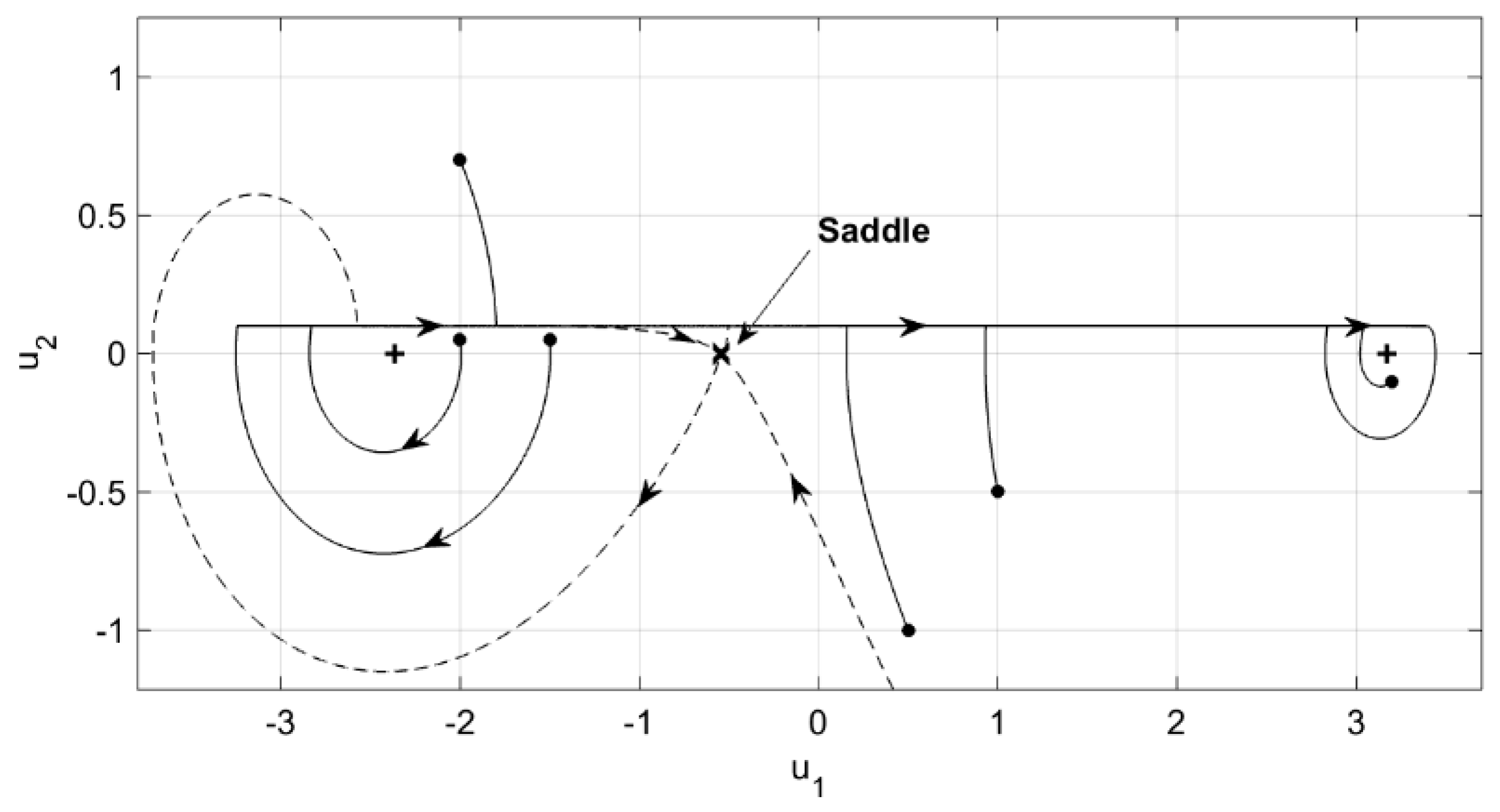
7. Spiral Source–Saddle–Spiral Sink

It was shown earlier that in a specific range of belt velocity, the right-side spiral becomes stable while the left-side spiral remains a source, as illustrated in Figure 3. Figure 6a depicts the phase portrait of the system. The equilibrium point on the right was stable and enclosed by an unstable limit cycle, shown as a thick solid line in Figure 6b. Thus, for initial conditions inside the limit cycle, the system response was asymptotically stable as the trajectory approached the right sink following a converging spiral. Outside the limit cycle, the system behavior was similar to that in Figure 5. That is, all trajectories eventually ended in the sustained stick-slip oscillation orbit shown in solid line, about the right-side equilibrium point.

For the current nonlinear model which possessed three equilibrium points, it was not possible to investigate the existence of limit cycle analytically. But since the divergence of the state vector changed sign in the domain of oscillation, according to Bendixson criterion, the occurrence of the limit cycle was possible. Investigating closed orbit around the spiral sink, a stationary amplitude of the limit cycle could be detected as verified by the results in Figure 6b.

8. Spiral Sink–Saddle–Spiral Sink

Further increase in belt speed yielded two spiral sinks flanking the saddle as suggested by Figure 3. Figure 7a depicts the phase plane trajectories in this case. Note that there were two unstable limit cycles, shown using thicker solid lines, each enclosing one of the spiral sinks, with the limit cycle on the right was slightly larger. Any initial condition within a limit cycle yielded an asymptotically stable response trajectory towards the corresponding equilibrium point, as shown in Figure 7b,c. On the left-side, the system attained a Sprag-slip configuration which yielded a self-energizing friction effect. On the outside of the limit cycles, the system behaved as described in Figure 5. The trajectories ended up in the stick-slip orbit shown as the thinner solid line about the right-side equilibrium point.

9. Case of One Equilibrium Point

Figure 8 shows the cases of a single equilibrium point. For relatively low belt velocity ($V=0.1$) the system yielded a spiral source (Figure 8a). The transient response is shown as dashed lines and the sustained oscillation as solid lines. Any initial condition, shown as dots, ended in the sustained stick-slip oscillation around the spiral. Figure 8b illustrates the phase plane for V = 0.5 where larger belt velocity resulted in Hopf-bifurcation, i.e., the spiral source transformed to a spiral sink, encircled by an unstable limit cycle shown using the thick line. Any initial condition grew or shrunk to the sustained stick-slip oscillation so long as it was outside the region enclosed by the limit cycle. An initial condition in the region within the limit cycle yielded an asymptotically stable system response, as shown in Figure 8b. The observed Hopf-bifurcation was consistent with that found in Refernce [24], wherein, it is shown to be the result of exponentially decaying friction coefficient.

10. Discussion

Numerical studies showed that no matter what the initial condition was, the oscillator was going to experience steady-state oscillation around the right-hand side equilibrium point. It should be noted that choosing a proper time-step was crucial to achieving correct numerical results, otherwise, incorrect trajectories showed up such as overshoot or steady-state stick-slip orbits around the left spiral. Therefore, it was necessary to verify the accuracy of the results. No matter where the oscillator stuck to the belt, it moved with the belt velocity as long as the friction force was less than its maximum static value. Stick to slip transition took places when friction force reached its maximum and either the tangential pushing or pulling elastic force overcame the static friction force. By assuming that the system was in stick phase (${\mathrm{u}}_2=V$ and $\mathsf{\mu }={\mathsf{\mu }}_{\mathrm{s}}$), tangential net force (${\mathrm{F}}_{\mathrm{net}}$) on the oscillator iwas plotted for a given set of parameters (Figure 9). As long as ${\mathrm{F}}_{\mathrm{net}}<0$, it meant the elastic and damping forces were less than maximum friction force and the system kept stick phase. Stick to slip transition happens when ${\mathrm{F}}_{\mathrm{net}}=0$, in other words, friction force reaches its maximum value [25]. For $\mathsf{\alpha }\le 3$, the curve just crossed the thick horizontal dashed line one time (${\mathrm{F}}_{\mathrm{net}}=0$) on the right-hand side of the right spiral (Figure 2c and Figure 9).

Another question that may arise is the possibility of overshoot in the system, when the oscillator moves faster than the belt. Thomsen and Fidlin discussed that the overshoot cannot occur during the steady-state oscillation in a convenient mass-on-belt system [26]. Though, in the current model, the spring was compressed around the origin. Therefore, the possibility of overshoot at some point between the origin and the right spiral should be investigated. By considering net force on the oscillator, the onset of overshoot during the transient response, if occurs, is in the range of $u_1\in \left[{\mu }_s,\sqrt{{\alpha }^2-1}\right]$ and $u_2=V$. The lower range of $u_1$ will increase, i.e., the range gets tighter, if $n>0$. But the upper limit is always fixed. For the given range of parameters in the current study, i.e., n = 1, $\zeta =0.01$ and $V=0.5$, it could be easily seen that the maximum friction force was always dominant in the range of possible overshoot (Figure 9). Consequently, the possibility of overshoot was ruled out in the current problem. Though, for different sets of spring/damper configurations or specific choice of parameters overshoot may take place [18].

The unstable limit cycles which enclosed the spirals are shown in Figure 10. As it can be observed the amplitude of the both limit cycles decreased as the belt slowed down untiel the limit cycles vdanish and the origins became unstable, i.e., Hopf-bifurcation happened. The Hopf-bifurcation occured for the right spiral at $V\approx 3.2$, while the left one was still unstable (Figure 3 and Figure 10). Increasing the belt velocity to $V\approx 3.5$, both spirals experienced Hopf-bifurcation. Due to the complexity of the nonlinear equation of motion, numerical methods were employed to capture limit cycles. The existence of a limit cycle, locating it and investigating its existence have been widely discussed by researchers [27,28].

The system was studied numerically to investigate its global behavior. It was shown that one spiral point was always dominant. The direction of motion of the belt pointed to the dominant spiral point. Varying the belt speed yielded the three scenarios:

• Spiral source–saddle–spiral source at a relatively low belt speed.
• Spiral source–saddle–spiral sink at an intermediate belt speed.
• Spiral sink–saddle–spiral sink at a relatively high belt speed.

Any initial condition in the phase plane in Scenario 1 resulted in a unique sustained stick-slip oscillation orbit around the dominant spiral on the right-side. For intermediate belt speed, Scenario 2, Hopf-bifurcation occurred for the right spiral. Consequently, the dominant spiral source on the right-side was transformed to a spiral sink with an accompanying encircling unstable limit cycle. For any initial condition outside the limit cycle the response was similar to Scenario 1. For an initial condition within the limit cycle, the system response was asymptotically stable and approached the respective sink. Relatively high belt speed converted the left-side spiral source to a spiral sink and an encircling unstable limit cycle. In this case, two small regions in the phase plane were created around each sink bounded by its respective limit cycle. For any initial condition chosen within these regions, system response was asymptotically stable. Choice of the initial condition within the left-side limit cycle led to Sprag-slip response.

11. Conclusions

A horizontally moving mass suspended above by a linear spring-dashpot combination was used to investigate friction-induced instability in a pseudo-rigid-body representation of a bi-stable compliant mechanism. Frictional input provided by a moving belt included the Stribeck effect through an exponentially decaying friction coefficient as a function of sliding velocity. Due to the large deflection of the mass giving rise to geometric nonlinearity, the inclusion of the Stribeck effect of the friction coefficient and variability of the contact force, the resulting friction force was found as a function of the system states, namely, slider velocity and position.

The system was shown to possess one or three equilibrium positions that depended on the range of dimensionless normal force and pre-compression ratio. Eigenvalue analysis was performed to examine the behavior of the linearized system in the vicinity of each equilibrium point. It was shown that, though viscous damping altered the friction force, it could have a stabilizing effect on the system near spirals.

Normal force and spring pre-compression were bifurcation parameters that could lead to pitchfork-bifurcation. Increasing belt velocity caused a subcritical Hopf-bifurcation, in which, a spiral source at the equilibrium point transformed to a spiral sink and formation of an unstable limit cycle encircling it. Such bifurcation occurred for the right-side equilibrium point at a lower belt speed than that for the left-side spiral. It was found that the disparity in velocity corresponding to the two bifurcations increased with an increase in damping ratio.

Finally, it was proven that overshoot and mass-belt detachment were not possible for the current model. In addition, the stick-slip transition was discussed in detail to explain the reason why the stick-slip loop did not occur around the left spiral.