Abstract
This research aims to analyze the vibration response of damaged rolling element bearings experimentally and to assess their degree of degradation by examining parameters extracted from the time domain. This task was accomplished in three phases. In the first phase, a test rig was carefully designed and precisely manufactured. In particular, an innovative solution for rapidly mounting and dismounting bearings on the supporting shaft was tested and used successfully. In the second phase, a specific technique of seeding defects inside the ball bearings was developed. In the last phase, damaged bearings (and healthy ones serving as a reference) were installed on the test rig, and different vibration measurements were taken. The results obtained from this work show that different parameters could be extracted from the time domain. In addition to the six common indicators (peak, root mean square, crest factor, kurtosis value, impulse factor, and shape factor), four hybrid new ones have been proposed (Talaf, Thikat, Siana and, Inthar). The experimental results confirm the well-known efficiency of kurtosis in the detection of bearing defects. However, the newly proposed parameters were found to be more responsive to defect growth.
1. Introduction
Rolling element bearings, also known as anti-friction bearings, are essential mechanical components for all types of rotating machinery, from small hand-held devices to heavy-duty industrial systems. Although rolling bearings are manufactured with maximum care using high-precision techniques, they may develop defects early during their usage depending on the nature of the operating parameters and the working environment. In an attempt to be more competitive, manufacturers are pushing production machines to their operating limits, which affects the longevity of their bearings. The condition and health of the bearings play a crucial role in the functionality, availability, and performance not only of the bearings themselves but also of the machines on which they are mounted. Any possible damage or fault in the bearing systems can quickly develop into a dangerous failure mode without any vital warning signs. The consequences can range from minor irritation (e.g., noise, discomfort, or vibration) to the failure of an entire machine or production line, resulting in significant losses of profit or, in extreme cases, human life. The statistics for bearing imports/exports [1], displayed in Table 1, highlight two facts. First, the import/export of bearings has significantly increased during the last ten years. A few of the imported bearings are used for the initial mounts in building new machines, while the rest are used to replace damaged ones following catastrophic failures. Second, the high consumption of bearings is not limited to specific countries exclusively but is a problem in all of them. Surprisingly, recent statistics from the industry sector in the United States (US) [2] confirm that between 30% and 50% of self-induced failures are the result of maintenance personnel not knowing the basics of maintenance. Moreover, up to 90% of companies in the US do not follow best maintenance repair practices. This negligence or ignorance in the use of bearings explains why the failure of these elements is a common problem for maintenance practitioners worldwide.

Table 1.
Importation of ball or roller bearings by country between 2001 and 2016 [1].
The causes of unwanted vibrations in rolling element bearings range from faulty installation and poor handling [3] to surface fatigue [4]. Over time, the under-surface fatigue process leads to the formation of various defects [5] within bearings. When repeated cycles of stress between rolling elements inside a bearing exceed the endurance limit of the metal, fatigue cracks appear on the surface. These defects and cracks propagate and result in substantial pits or spalls on the surface of the bearing components. When a rolling element rolls over a spall, it generates an impacting force. These periodic impacts occur at the frequency at which the balls cross the spall. The repetition rates of these events are called characteristic defect frequencies. Their values depend on the geometry and the rotational speed of the bearing [6]. When the excitation energy created by such impacts is high enough, it may excite the resonance frequencies of the rolling element bearing system [7].
Rolling element bearings frequently experience vibrations because of their inherent non-linearity. This behavior can arise from a Hertzian load-deformation relationship, varying compliance, clearances, local and distributed defects, etc. The vibration signals generated by rolling element bearings tend to be complicated and are influenced by several factors, notably lubrication, load, geometry, and the presence of faults.
The identification and detection of damage through changes in the vibration characteristics of a system have been the subject of much research over the last 20 years, and numerous models (theoretical, numerical, and hybrid) together with damage identification algorithms have been proposed for detecting and locating the damage in structural and mechanical systems. In general, fault severity identification algorithms can be categorized into model-based approaches and data-driven approaches. The model-based methods depend on a fundamental understanding of the physics of the process [4,5,6]. In data-driven methods, features can be extracted to present the historical process data as a priori knowledge of a diagnostic system [3,7,8,9]. The detection of a bearing defect is the first step in the diagnosis process. However, the prediction of the growth rate of bearing defects as well as the bearing’s remaining life are also crucial.
Since the early 1950s, many researchers have assisted our understanding of the vibration responses of non-defective (healthy or intact) and defective bearings. Several studies have been published on various theoretical, numerical, and experimental approaches. For instance, McFadden and Smith [8,9] formulated the impulses caused by point defects as a series of repeated force excitations. Tandon and Choudhury [10,11] described the impulses generated by a surface-localized defect as triangular, rectangular, and half-sine force excitations. Kiral and Karagulle [12,13] modeled the induced impulse as a rectangular force excitation. Sassi et al. [14] formulated the impulse caused by the localized surface defect as sinusoidal and rectangular force excitations. Behzad et al. [15] described the impulse caused by a localized surface defect as a stochastic excitation force.
On the experimental side, because the vibration signals produced by other problems such as poor balance, misalignment, or damaged gears are always blurring those coming from damaged bearings, researchers and engineers quickly understood that the acquisition of vibration data is a challenging exercise ranging between science and art. Bearings can be monitored by using simple methods or other more complicated ones that require sophisticated signal processing algorithms. To enhance weak signatures coming from noisy signals, scientists have proposed different signal processing techniques. These include high-frequency resonance techniques [16], spectral kurtosis [17], wavelet analysis [18,19], empirical mode decomposition [20], cyclo-stationary approaches [21], minimum entropy deconvolution [22], stochastic resonance [23], and some other innovative approaches [24]. Many of these techniques are processed in the frequency domain and are not always easy to obtain because of the non-linear behavior of the machines. In such cases, it is difficult to extract information from the frequency domain representation, since traditional spectrum analysis applies to mechanical structures with linear dynamic behavior. On the other hand, vibration-monitoring methods based on structural vibration signals from the time domain have been gaining popularity recently. These techniques are mostly based on statistical features and do not assume any model or linearity of the machine under investigation.
Obviously, the time domain and the frequency domain are two powerful tools that have different advantages and disadvantages. Usually, novice users keep wondering what kinds of problems and situations are better analyzed with the time domain or frequency domain plots. However, the primary challenge remains: how much technical background does one need to carry out a successful analysis? The investigation in the frequency domain is usually more powerful for detecting nascent problems, for locating the origin of a problem, or for distinguishing between two different issues. However, before getting such results, one should ask what the sampling frequency is? What should the minimum time of acquisition be? What kind of filters should be used? How should the frequency range for an accurate analysis be set? With similar confusing questions arising with each investigation, vibration analysis has been restricted exclusively to scientists or highly skilled technicians. What ordinary users are looking for is a straightforward process in the time domain, where they feed the signal into any statistical or mathematical software package (Matlab, Excel…) and obtain some easily interpreted and unambiguous condition indicators, or defect severity indices that can be calculated from the statistical parameters of the extracted vibration signature. Such useful time-domain metrics will serve as a dashboard for managers to track defect growth, to provide a means to define acceptable and unacceptable machine conditions, and to decide the appropriate time to stop production and replace a damaged bearing that was detected a long time previously.
Research is at its most useful when it can make reliable predictions based on experimental observations and generate useful and practical results that can be used by everyday users. Therefore, in this research paper, we aim to bring more insight into the vibration response of damaged bearings in the time domain based on experimentally obtained data. In particular, we intend to investigate the influence of an increase in bearing damage with respect to the variation in time-domain scalar indicators and their ability to trace the increase in the size of localized defects.
This article is structured as follows. Following the introduction in Section 1, Section 2 describes the test rig’s design and manufacture. The insertion of defects into the outer and inner rings (raceways) of the bearings is explained in Section 3. The data acquisition process is detailed in Section 4, and our discussion and interpretation of the results are presented in Section 5. Section 6 presents some conclusions drawn from the research.
2. Experimental Setup
The first challenging task in the present work was the development of a test rig to fulfill the requirements of the current investigation. The experiments in this type of research require the seeding of defects of various sizes and locations, the repeated mounting and dismounting of the test bearings, the application of different speed and load running parameters, and the acquisition of vibration signals. Our test rig was designed to meet these conditions and to imitate industrial ball bearing applications. The system consists of four functions: the driving function, the supporting function, the loading function, and the vibration measurement function.
2.1. The Driving Function
The driving function consisted of a three-phase alternating current motor, whose input frequency was controlled by a variable frequency drive (brand: CHZIRI, Model: ZVF9V-G0110T4MDR, Zhejiang, China). The motor used in this experiment supplied 2.2 kW (3 Hp) at a maximum speed of 2840 rpm.
2.2. The Supporting Function
The supporting function of the test rig was provided by four major components: a shaft, a housing, a tailstock equipped with a live lathe center, and a support base. Two supporting bearings, mounted inside a sealed housing, carried the shaft. The housing inner cavity was filled with 650 mL of light hydraulic fluid to lubricate the support bearings. At the other end, the tailstock protected the shaft from any bending that may have resulted from any excessive external radial load.
2.2.1. Shaft Design and Housing Assembly
The shaft was fabricated from AISI 304 annealed stainless steel. It was designed to be linked on one side to the motor by a flexible rubber coupling. The other side of the shaft was provided with two perpendicular grooves, conically drilled in the center, and held by a live lathe center and a tailstock. The shaft was held by two support bearings, which were embedded inside a housing. A spacer tube, as shown in Figure 1, separated the two support bearings.
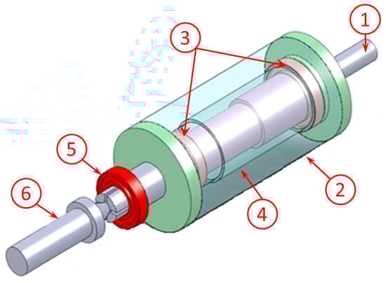
Figure 1.
Housing assembly: (1) main shaft; (2) housing; (3) support bearings; (4) spacer; (5) test bearing; (6) tailstock and live lathe center.
Bearings are usually fitted with an interference fit (forced mounting of type H7m6 or H7p6) on one race and a sliding fit on the other (of type H7h6 or H7g6). If the shaft is rotating and the housing is static, then the junction between the inner ring and the shaft will be forced while the one between the outer ring and the housing will be sliding. Frequent mounting and dismounting of a bearing that is mounted with an interference fit on its supporting shaft is a difficult and time-consuming procedure that, if repeated, may permanently damage the bearing or the shaft or even both of them. Therefore, an innovative solution based on an expandable elastic end was adopted (Figure 2). By making two perpendicular cuts on the tip of the shaft, local elasticity was created, which permitted us to introduce the bearing and lock it in place by inserting a tapered screw inside the threaded axial hole.
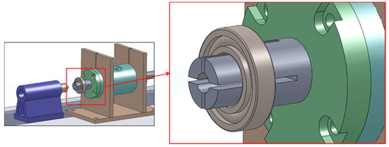
Figure 2.
The expandable elastic end for repeated mounting/dismounting of the bearing.
2.2.2. Tailstock and Live Lathe Center
A tailstock equipped with a live (rotating) lathe center was used in this test rig for two purposes:
- To prevent the rotating shaft from bending: since the test bearing is located at the end of the shaft (a cantilevered position), beyond the span of the two supporting bearings, there is always a risk of deformation of the shaft when the radial load applied is excessive, and,
- To push on the elastic end of the shaft and make it expand or retract, and hence make the locking of the bearing at its support easier and faster.
2.2.3. Support Base
A square steel support base (1 m × 1 m × 2 cm) held all the test rig components together. Three U-shaped steel beams were welded to the support base to prevent it from bending. A total of six anti-vibration rubber pads was also fitted to these beams to dampen the generated vibrations, as shown in Figure 3.
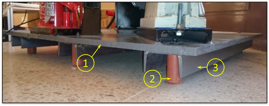
Figure 3.
Support base system: (1) 1 m × 1 m × 2 cm supporting plate; (2) 6× anti-vibration rubber pads; (3) 3× U-shaped steel beams.
2.3. The Loading Function
As shown in Figure 4, the loading function’s primary role was to apply a radial load on the test bearing. It consisted of a hydraulic jack (1), a lever (2), and a load cell (3).
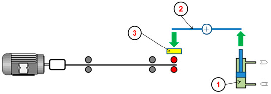
Figure 4.
Hydraulic loading system: (1) hydraulic jack; (2) lever; (3) load cell.
When the hydraulic jack was activated, its piston pushed on a rectangular steel bar used as a lever, which was free to turn about a fixed support. As shown in Figure 5, the force applied to the lever was transferred to the test bearing through a load cell mounted on a special base. The sensor-mounting base consisted of a round disc 10 cm in diameter, on which an accelerometer was installed alongside the load cell (Figure 6).
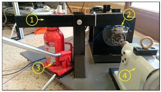
Figure 5.
Loading system: (1) lever; (2) load sensor; (3) hydraulic jack; (4) tailstock.
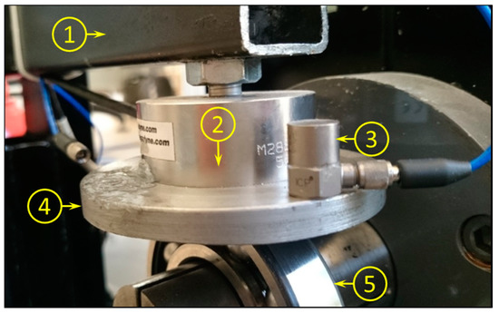
Figure 6.
Sensor mounting device: (1) lever; (2) load sensor; (3) accelerometer; (4) mounting base; (5) test bearing.
2.4. Vibration Measurement Function
The vibration signal was acquired by using a high sensitivity, ceramic shear ICP® accelerometer (from PCB Piezotronics, Model No. 352C33, 100 mV/g, Depew, NY, USA), which was directly fixed on the same mounting base that supported the load cell (from Omegadyne Inc., Model No. LCM204-50KN, Manchester, UK). The readings were controlled by a four-channel NI-9234 sound and vibration input module at a sampling frequency of 51.2 kHz during a time interval of 10 s for each acquisition. In the final stage, all the electrical connections were fixed, the test rig was painted, and the motor was aligned with the shaft. The manufactured test rig at its final stage is shown in Figure 7.
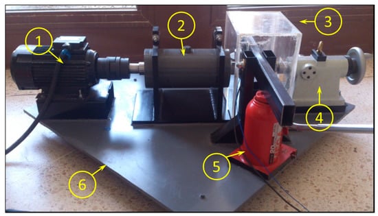
Figure 7.
The manufactured test rig with a protective box: (1) motor; (2) housing; (3) protection cover; (4) tailstock; (5) hydraulic jack; (6) base.
A protective safety box made of an acrylic sheet was specially manufactured to cover the test bearing during the experiments and to protect the user from any disconnected flying objects.
3. Defect Insertion
3.1. Dismounting the Bearings
The test bearings used in this research were of the deep-groove ball bearing type ((Nihon Shinbun Kyokai) NSK 6208). To dismount the different parts of the bearings, the heads of their rivets were simply removed by drilling through each of them (Figure 8a). To avoid deformation of the cage during the drilling process, a special mold was prepared from epoxy clay (made by combining resin and hardener) to support the bearing correctly (Figure 8b).
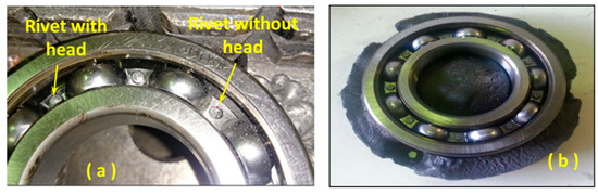
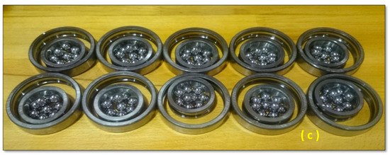
Figure 8.
Dismounting of bearings. (a) rivet head removal; (b) epoxy clay mold used to hold the bearing cage; (c) fully dismounted bearings.
3.2. Controlled Defect Insertion: Impacting System
In real situations, the defects that occur in bearings are usually encountered on both rings. Therefore, an impacting system was designed and manufactured to seed defects on both the outer and inner raceways. The system transmitted the energy of a falling mass to a sharp conical tool that punched a hole in the impact surface. The tool used for this purpose was a tungsten carbide-tipped dead center that is commonly used in lathe machines (Figure 9).
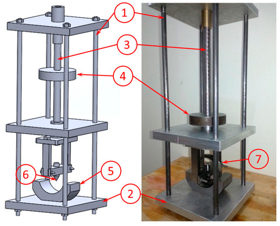
Figure 9.
The impacting system: (1) four supporting columns; (2) three supporting plates; (3) graduated guiding bar; (4) falling mass; (5) ring support; (6) sharp conical punch; (7) bearing ring.
To control the size of the seeded defects, the relationship between the mass value, its drop height, and the defect size needed to be understood beforehand. Therefore, to fit correctly inside the device, three different masses were manufactured (0.666 kg, 1.408 kg, and 2.843 kg). Each one of these masses had to be dropped from various heights. The combination of all previous masses, together with their drop heights, permitted us to generate the calibration curve displayed in Figure 10.
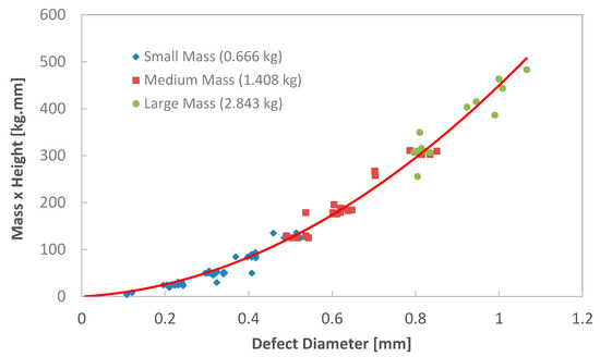
Figure 10.
Defect insertion calibration curve.
After seeding the defects, a Universal Serial Bus (USB) digital microscope was used to control their sizes (Figure 11). The observations showed that the method was able to generate defects at an accuracy of 15%, relative to the predicted defects based on the calibration curve.
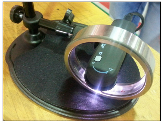
Figure 11.
Microscopic observation of the defects.
3.3. Remounting the Bearings
Once the defects were correctly seeded into appropriate locations, the bearings were reassembled back into their original configurations. To avoid any possibility of inadvertent opening, a set of 3.2-mm rivets were used to close the bearing cages (Figure 12b). Finally, the mounted bearings were lubricated and tagged (Figure 12c). During all these steps, particular effort was made to keep the balls safe and clean to avoid any damage or scratching that may have affected the overall vibration response of the bearing when remounted.
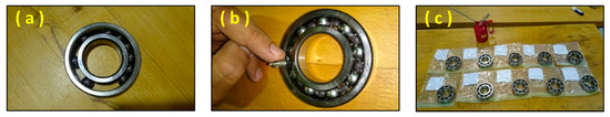
Figure 12.
Remounting of the bearings: (a) insertion of the balls between the inner and outer rings; (b) riveting of the cage; (c) lubrication and storage.
4. Methodology and Experimental Investigation
The experiments were conducted for three healthy bearings and 16 defective ones. Eight bearings had defects inserted into their inner rings, and another eight bearings had defects inserted into their outer rings. As displayed in Table 2, the defects ranged from 0.35 mm to 2.0 mm in diameter.
Table 2.
Defect sizes on the outer and inner rings.
During the experimental investigation, each test was repeated ten times to reduce random interference and enhance the reliability of the acquired data.
4.1. Time Domain Waveform
When a defect is found on the outer ring of a bearing, and that particular ring is stationary, the defect will be located inside the stress zone the entire time (Figure 13a). When balls roll across defects of this type, they will produce a set of impulsive forces with equal amplitudes (Figure 13b). Consequently, the waveform of the vibration response will be repeated identically each time the ball strikes the defect (Figure 13c). This cyclic signature could be used to pinpoint the location of faults on a fixed ring of a damaged bearing.
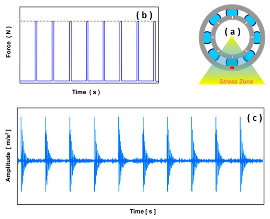
Figure 13.
Typical case of localized damage on the outer race: (a) location of damage on outer race, which is stationary; (b) pattern of impacting force; (c) time response waveform.
When the defect is located on the inner ring, and that specific ring is rotating, the defect will be moving episodically in and out of the stress zone (Figure 14a). Consequently, the point at which the rolling elements encounter the defect will keep moving from one position to another, and the resulting impact forces will be modulated (Figure 14b). Because of this, the time waveform will also be modulated (Figure 14c).
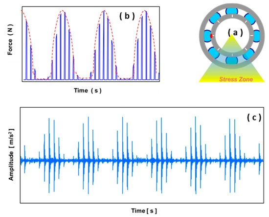
Figure 14.
Typical case of localized damage on the inner race. (a) Location of damage on inner race, which is rotating; (b) pattern of impacting force; (c) time response waveform.
4.2. Health Indicators and Vibration Analysis
The supervision and monitoring of a machine’s condition require investigators to choose a particular number of indicators ahead of time. An indicator arises from a parameter that can be acquired when the machine is running and must clearly reflect the state and performance of that machine. The evolution of these indicators over time is indicative of the appearance or aggravation of a defect.
4.3. Time Domain Analysis
Time domain analysis is considered to be the easiest and simplest technique for analyzing vibration signals. This technique can pinpoint the presence of defects inside bearings but, unfortunately, in some cases, it does not give information about the location of the defect (e.g., the inner race, the outer race, the cage or the rolling element). For example, in the case of two different bearings with different sizes and different locations, the distinguishing and recognition of the damaged bearing from the healthy one is an easy and straightforward task in the frequency-domain since their frequency families are different and appear distinctly from each other on the same spectrum. However, in the time-domain, because of the different locations of both bearings with respect to the same accelerometer, their phase components may be different from each other, and consequently, the summing of both signal may be not recognizable. The troubleshooting in the time domain is in general a challenging task that requires extra skills not always in the reach of common users.
To monitor the effect of increasing defect sizes on the bearings’ vibration responses, several statistical parameters extracted from the time domain have been reported in the literature [25]. In general, an indicator’s value does not have fundamental significance. However, its evolution over time is usually indicative of the occurrence or propagation of a defect. The six statistical scalar parameters most commonly used for diagnosing bearing faults are maximum or peak value (MAX or PEAK), root mean square (RMS), crest factor (CF), kurtosis value (KU), shape factor (SF), and impulse factor (IF) [26]. Table 3 shows the definitions of these parameters.
Table 3.
Time domain indicators used for detecting bearing vibrations.
5. Results and Discussion
The principles and procedures of the analytical methodology are depicted in Figure 15. First, a healthy bearing free from any surface defects was mounted on the test rig, and its vibration signals were acquired, analyzed, and stored. The time domain parameters extracted from the healthy bearing’s vibration data served as a reference for further signal processing efforts. Next, the healthy bearing was removed and replaced on the test rig by a defective one. Again, the time-domain parameters were recorded and analyzed. Since the vibration signal emanating from the bearing passes through the machine to reach the sensor, it is evident that the contribution of the machine, with all its imperfections, will be visible in all the measurements, regardless of whether the test bearings installed on the rig are healthy or damaged. The ability of the statistical time-domain parameters to detect or quantify bearings faults would lack accuracy because such parameters are likely to be strongly influenced by non-bearing faults such as electrical problems, shaft imbalances, pitting on the gear tooth, or misalignment. In particular, when the defect is newly created, its vibration pattern may not be precisely identifiable among all the inputs generated by the neighboring mechanical components. To enhance the visibility of the bearing’s vibrations, the disturbing effect of the machine should be canceled, if possible, or minimized, at the very least. This aim could be achieved by performing a spectral subtraction between the first spectrum collected from the machine holding a healthy bearing, and a second spectrum from the same machine but with a defective bearing. Of course the previously mentioned subtraction would be possible only in the frequency-domain, again because all the frequency components are distinct in that case. The result of this procedure should theoretically cancel or reduce the effect of the hosting environment (present in both spectra) and leave the effect of the damaged bearing alone. Returning back to the time-domain would theoretically generate statistical parameters that are more stable and less sensitive to the machine contribution.
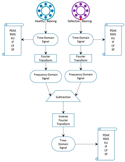
Figure 15.
Flow diagram of the experimental method.
5.1. Evolution of Time Domain Scalar Parameters
The variations of the two statistical parameters PEAK and RMS (presented in Table 3) are plotted, as an example, in Figure 16. The PEAK value could be measured in either the time domain or the frequency domain. It is the maximum acceleration in the signal amplitude. Both PEAK and RMS values increase as fault sizes grow. However, in the early stages of bearing degradation, the RMS value does not change so quickly. In order to quantify the dependence relationship between the increase in damage size and these parameter values, we analyzed this relationship via the regression model, shown on top of each curve. Based on the displayed equations, it seems that the evolution of PEAK is more linear than quadratic.
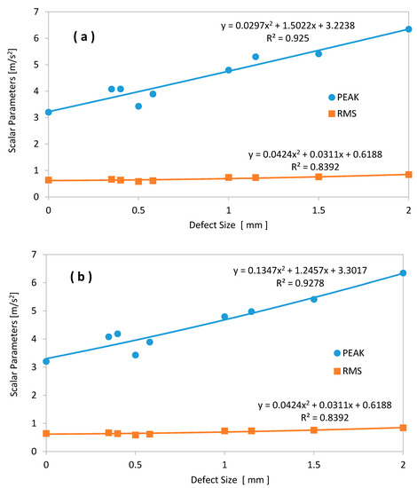
Figure 16.
Evolution of the scalar values peak value (PEAK) and RMS: (a) defects on the inner bearing race; (b) defects on the outer bearing race.
Even though the actual values of the different health indicators are meaningful, their degrees of change are much more important. Therefore, to make a direct comparison of the trend of each indicator, their values should be divided by their initial values (obtained from the reference, i.e., the healthy bearings). Consequently, in all the following graphs, the parameters have unity as the starting value. This process is known as “normalization” and allows for better comparisons of the evolution of the parameters. The new “normalized” PEAK and RMS parameters are displayed in Figure 17. One can see that, in contrast to the amplitude of RMS, PEAK is much more sensitive to increases in the size of the damage.
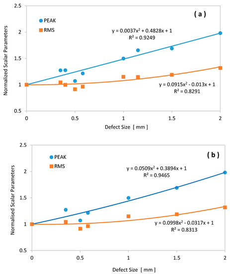
Figure 17.
Evolution of normalized PEAK and RMS values: (a) defects on the inner bearing race; (b) defects on the outer bearing race.
5.1.1. Inner Ring Defects
The evolutions of other time-domain parameters (KU, IF, CF, and SF) versus the size of the defects seeded on the inner ring are portrayed in Figure 18, from spall initiation (zero defect size) up to a defect 2 mm in diameter. These data were collected from test bearings damaged on their inner rings, at a speed of 800 rpm, and an external load of 0.5 kN. One can see that KU, PEAK, and CF were the most sensitive parameters (i.e., they had the highest rate of change) to an increase in defect size on the inner ring.
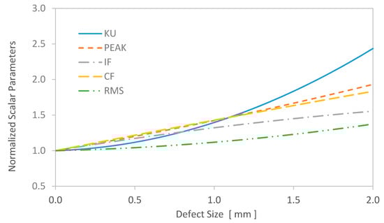
Figure 18.
Evolution of time-domain parameters with respect to inner ring defect size.
5.1.2. Outer Ring Defects
For the case where the defects were located on the outer ring, the changes in the normalized scalar parameters are plotted in Figure 19. This result was again obtained under a specific rotation speed of 800 rpm and an applied load of 0.5 kN.
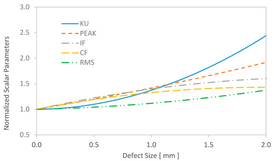
Figure 19.
Evolution of time-domain parameters with respect to outer ring defect size.
At first glance, the normalized curves indicate that KU appears to be the most sensitive time domain parameter to increases in defect size, regardless of whether the defect is located on the outer race or the inner race. This finding is in good accordance with previously published work [26].
When a comparison is made between outer ring defects and inner ring defects, the extracted parameters have similar degrees of sensitivity, contrary to what was previously expected. Usually, when the defect is located on the outer race, the sensitivity of the time-domain parameters is higher. This is probably caused by two main factors:
- When a defect is located on the inner ring, as displayed in Figure 20, the vibration wave should travel through a relatively long path to reach the sensor. As it moves through the different interfaces, the energy of the signal is considerably dampened. On the other hand, if the defect is on the outer ring, the transmission path is considerably shorter. Therefore, the signal energy coming from the outer ring is higher.
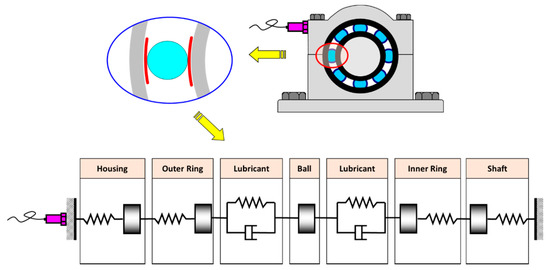 Figure 20. Effect of the vibration wave’s path length on accelerometer readings.
 - When the defect is located on an outer ring that is fixed, the defect remains inside the load zone for a longer time. On the other hand, when the defect is located on a rotating inner ring, the defect will cross the load zone once every cycle and only for a short time.
In this research, a comparison between Figure 18 and Figure 19 shows that no significant difference was found between the cases where the defects were located on the outer ring and when the defects were on the inner ring. This is probably because the applied load was not high enough to magnify the effects of the outer ring defects. As a matter of fact, because the testing procedures were made over long periods of time (17 bearings in total and 10 readings for each case) and to avoid damaging the main machine shaft, the radial load was considerably reduced. The applied load (~0.5 kN) was only just enough to close the internal bearing clearance and prevent rotation of the outer ring.
5.2. New Time Domain Parameters
All the parameters presented above showed an increase with respect to the evolution of defect size but at different rates of sensitivity. In general, KU and PEAK were the most sensitive indicators of the evolution of any defects inside the bearing. In the first stage of degradation, PEAK was more responsive to the increase in damage size. However, at later stages, KU became more dominant and quickly took the lead over all other parameters. Since the sensitivity of the parameters was variable throughout the duration of the bearing test, one might wonder whether their combination with any other mean value would generate a better parameter with higher sensitivity. In a previous paper [26], the introduced parameters Talaf and Thikat were found to be more efficient for monitoring the health condition of damaged bearings. The same parameters were tested again in this investigation, together with two new parameters, called Siana and Inthar. The definitions of these four new parameters are listed in Table 4.
Table 4.
New time domain parameters.
The evolution of the new parameters is presented in Figure 21 and Figure 22 for outer and inner ring defects, respectively.
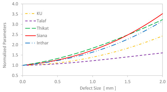
Figure 21.
Evolution of the new time domain parameters with respect to the size of the inner ring defects, in comparison with kurtosis.
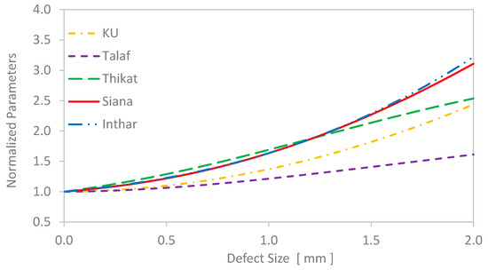
Figure 22.
Evolution of the new time domain parameters with respect to the size of outer ring defects, in comparison with kurtosis.
6. Conclusions
This research presents an experimental study to investigate the vibration behavior of defective bearings by using an efficient test rig that was specially designed and manufactured for this purpose. A practical method of opening bearings, seeding defects, and dismounting and remounting bearings was used efficiently to insert surface defects with diameters ranging from 0.35 mm to 2.0 mm. By deliberately adding defects of different sizes on the raceways of a deep-groove ball bearing, several experiments were conducted to recognize and quantify the existence of these defects from the vibration signal. To keep monitoring the evolution of the defects, various parameters extracted from the time domain were considered. They all showed a noticeable relationship with the growth in defect size but at different degrees of sensitivity. The most sensitive ones were found to be the kurtosis value and the peak amplitude. In addition to the conventional time-domain parameters commonly used by vibration analysts, two new time-domain parameters were introduced. These were named SIANA and INTHAR. Both of these demonstrated high sensitivity to growth in the size of bearing defects. In conclusion, this study has the potential to offer vibration analysts a broad list of parameters that may be used as a control panel for the early detection of bearing faults.
Author Contributions
The test rig was designed by S.S. and manufactured by A.S. The experiments were performed by A.S. and A.A. The data were analyzed by S.S. and J.R., S.S. wrote the paper.
Funding
This research was funded by the College of Engineering at Qatar University, grant number QUST-CENG-FALL-14/15-3.
Conflicts of Interest
The authors declare no conflict of interest.
References
- International Trade Center. Trade Map. Available online: http://www.trademap.org/tradestat/ (accessed on 2 August 2018).
- Smith, R.; Mobley, R.K. Industrial Machinery Repair: Best Maintenance Practices Pocket Guide; Butterworth-Heinemann: Oxford, UK, 2003. [Google Scholar]
- Howard, I. A Review of Rolling Element Bearing Vibration: Detection, Diagnosis and Prognosis; Tech. Rep. DSTO-RR-0013; Defense Science and Technology Organization: Melbourne, Australia, 1994.
- Halme, J.; Andersson, P. Rolling contact fatigue and wear fundamentals for rolling bearing diagnostics—State of the art. Proc. Inst. Mech. Eng. Part J. J. Eng. Tribol. 2010, 224, 377–393. [Google Scholar] [CrossRef]
- Rycerz, P.; Olver, A.; Kadiric, A. Propagation of surface initiated rolling contact fatigue cracks in bearing steel. Int. J. Fatigue 2017, 97, 29–38. [Google Scholar] [CrossRef]
- Sassi, S.; Badri, B.; Thomas, M. Tracking surface degradation of ball bearings by means of new time domain scalar indicators. Int. J. COMADEM 2008, 11, 36–45. [Google Scholar]
- Qiu, H.; Lee, J.; Lin, J.; Yu, G. Robust performance degradation assessment methods for enhanced rolling element bearing prognostics. Adv. Eng. Inf. 2003, 17, 127–140. [Google Scholar] [CrossRef]
- McFadden, P.D.; Smith, J.D. Model for the vibration produced by a single point defect in a rolling element bearing. J. Sound Vib. 1985, 96, 69–82. [Google Scholar] [CrossRef]
- McFadden, P.D.; Smith, J.D. The vibration produced by multiple point defects in a rolling element bearing. J. Sound Vib. 1985, 98, 263–273. [Google Scholar] [CrossRef]
- Tandon, N.; Choudhury, A. An analytical model for the prediction of the vibration response of rolling element bearing due to a localized defect. J. Sound Vib. 1997, 205, 275–292. [Google Scholar] [CrossRef]
- Tandon, N.; Choudhury, A. Vibration response of rolling element bearings in a rotor bearing system to a local defect under radial load. ASME J. Tribol. 2006, 128, 252–261. [Google Scholar]
- Kiral, Z.; Karagulle, H. Simulation and analysis of vibration signals generated by rolling element bearing with defects. Tribol. Int. 2003, 36, 667–678. [Google Scholar] [CrossRef]
- Kiral, Z.; Karagulle, H. Vibration analysis of rolling element bearings with various defects under the action of an unbalanced force. Mech. Syst. Signal Process. 2006, 20, 1967–1991. [Google Scholar] [CrossRef]
- Sassi, S.; Badri, B.; Thomas, M. A numerical model to predict damaged bearing vibrations. J. Vib. Control 2007, 13, 1603–1628. [Google Scholar] [CrossRef]
- Behzad, M.; Bastami, A.R.; Mba, D. A new model for estimating vibrations generated in the defective rolling element bearings. ASME J. Vib. Acoust. 2011, 133, 041011. [Google Scholar] [CrossRef]
- Dipen, S.S.; Vinod, N.P. A Review of dynamic modeling and fault identifications methods for rolling element bearing. Procedia Technol. 2014, 14, 447–456. [Google Scholar]
- Antoni, J. The spectral kurtosis: A useful tool for characterizing non-stationary signals. Mech. Syst. Signal Process. 2006, 20, 282–307. [Google Scholar] [CrossRef]
- Qiu, H.; Lee, J.; Lin, J.; Yu, G. Wavelet filter-based weak signature detection method and its application on rolling element bearing prognostics. J. Sound Vib. 2006, 289, 1066–1090. [Google Scholar] [CrossRef]
- Cui, L.; Huang, J.; Zhang, F. Quantitative and localization diagnosis of a defective ball bearing based on vertical-horizontal synchronization signal analysis. IEEE Trans. Ind. Electron. 2017, 64, 8695–8705. [Google Scholar] [CrossRef]
- Lei, Y.; He, Z.; Zi, Y. EEMD method and WNN for fault diagnosis of locomotive roller bearings. Expert Syst. Appl. 2011, 38, 7334–7341. [Google Scholar] [CrossRef]
- Antoni, J.; Bonnardot, F.; Raad, A.; El Badaoui, M. Cyclostationary modelling of rotating machine vibration signals. Mech. Syst. Signal Process. 2004, 18, 1285–1314. [Google Scholar] [CrossRef]
- Sawalhi, N.; Randall, R.B.; Endo, H. The enhancement of fault detection and diagnosis in rolling element bearings using minimum entropy deconvolution combined with spectral kurtosis. Mech. Syst. Signal Process. 2007, 21, 2616–2633. [Google Scholar] [CrossRef]
- Tan, J.; Chen, X.; Wang, J.; Chen, H.; Cao, H.; Zi, Y.; He, Z. Study of frequency-shifted and re-scaling stochastic resonance and its application to fault diagnosis. Mech. Syst. Signal Process. 2009, 23, 811–822. [Google Scholar] [CrossRef]
- Song, L.; Wang, H.; Chen, P. Vibration-based intelligent fault diagnosis for roller bearings in low-speed rotating machinery. IEEE Trans. Instrum. Meas. 2018, 67, 1887–1899. [Google Scholar] [CrossRef]
- Zhu, J.; Nostrand, T.; Spiegel, C.; Morton, B. Survey of condition indicators for condition monitoring systems. In Proceedings of the Annual Conference of the Prognostics and Health Management Society, Fort Worth, TX, USA, 27 September–3 October 2014. [Google Scholar]
- Sassi, S.; Badri, B.; Thomas, M. “TALAF” and “THIKAT” as innovative time domain indicators for tracking ball bearings. In Proceedings of the 24th Canadian Machinery Vibration Association Seminar on Machinery Vibration, Montréal, QC, Canada, 25–27 October 2006. [Google Scholar]
© 2018 by the authors. Licensee MDPI, Basel, Switzerland. This article is an open access article distributed under the terms and conditions of the Creative Commons Attribution (CC BY) license (http://creativecommons.org/licenses/by/4.0/).