Optimizing Fine-Tuning of Earth Foundation Models via Multidimensional Latin Hypercube Sampling for Small-Scale Burn Scar Identification

Abstract

Identifying small-scale burn scars is critical for global carbon accounting, yet remains computationally challenging due to spectral complexity and ground truth scarcity in heterogeneous landscapes. Conventional deep learning models often fail to generalize in such environments, lacking both domain-specific priors and representative training distributions required for precise segmentation. Here, we show that optimizing the fine-tuning of the Prithvi Earth Foundation Model (EFM) via Multidimensional Latin Hypercube Sampling (LHS) establishes a robust framework for this task. Our comparative analysis reveals that the domain-adapted Prithvi model achieves a Mean Intersection over Union (mIoU) of 0.91, outperforming standard Vision Transformers (ViT) by 31.9% and significantly surpassing reconstruction-based architectures, such as Scale-MAE. We demonstrate that LHS is superior to Simple Random Sampling (SRS) for optimizing foundation models, as it ensures statistical fidelity with a Kolmogorov–Smirnov (KS) statistic below 0.1 and effectively captures the tail distributions of fire weather indices. Furthermore, our framework exhibited exceptional data efficiency, retaining 94.5% of its peak accuracy with only 100 training samples. These findings provide a scalable solution for monitoring small-scale disasters in data-constrained regions and validate the synergy between rigorous sampling strategies and EFMs.

1. Introduction

Wildfires play a significant role in global ecosystem dynamics, with Africa contributing approximately 70% of the global annual burned area [1]. Despite this extensive coverage, accurate monitoring is challenging because of the prevalence of small fires covering less than 100 hectares. Global satellite observations have advanced our understanding through sensors such as MODIS and VIIRS [2], yet existing products such as MODIS MCD64A1 are limited by their coarse spatial resolution of 500 m [3]. This limitation causes a mixed-pixel problem, where the signal of a small burn is mixed with unburned vegetation, resulting in frequent missed detections [1]. Recent studies have indicated that overlooking these fires results in substantial uncertainties in burned area estimates and associated carbon emissions. For instance, in the fragmented landscapes of Sub-Saharan Africa, Sentinel-2 has been shown to detect approximately 80% more burned areas than coarse-resolution products [4,5]. Consequently, although high-resolution sensors such as Landsat and Sentinel-2 offer the necessary detail, relying on them individually often leaves gaps in temporal coverage. Therefore, the Harmonized Landsat Sentinel-2 (HLS) dataset proposed by [6], which combines both sources to improve observation frequency, is essential for the precise segmentation of burn scars.

Deep Learning architectures have become the standard approach to automate the interpretation of such high-resolution imagery [7]. Specifically, Convolutional Neural Networks (CNNs) [8], such as U-Net [9] and DeepLabV3+ [10], have improved detection boundaries [11,12,13]. However, the performance of these fully supervised models is often bottlenecked by the lack of diverse, high-quality labels [14]. Moreover, they face challenges in the temporal evolution of burn scars. Because burn signatures fade and vegetation regrowth occurs rapidly [15], burn scars can easily be confused with dark soils or wetlands [16]. Furthermore, models trained on curated datasets often perform poorly when applied to African savannas due to significant differences in vegetation structure and fire severity [14]. To address these limitations, EFMs, such as Prithvi [17], offer compelling solutions. By leveraging self-supervised learning (SSL) [18] strategies that combine Masked Autoencoding (MAE) [19] with ViT [20], these models extract rich feature representations from extensive unlabeled archives, thereby enhancing the detection of small and fragmented burn scars in complex landscapes.

Despite the robust pre-trained representations of EFMs, their effectiveness during the fine-tuning stage is contingent on the quality of the downstream training data [21]. This presents a critical yet frequently overlooked challenge in terms of sample representativeness. The prevailing practice often relies on SRS, which is not optimal for geospatial data. As environmental conditions and fuel types are spatially correlated, samples drawn from nearby locations often contain redundant information [22]. More critically, wildfires follow a long-tail distribution [23] driven by the complex interactions of environmental variables. SRS inevitably biases the training set towards average background conditions and systematically under-represents rare but critical cases, such as fires occurring under extreme weather [24,25]. Recent research suggests that training on such narrow distributions can cause models to fail unexpectedly when faced with broader or unseen contexts [26]. This sampling bias restricts the model’s ability to generalize, as it remains unexposed to the full physical range of fire regimes [27,28]. Therefore, optimizing sample selection to ensure comprehensive coverage is as crucial as architectural advancement [29].

To mitigate the limitations of SRS, this study proposes a fine-tuning strategy for the Prithvi model that prioritizes environmental representativeness over the training period. We employed Multidimensional LHS from [30] to construct a training set that uniformly covers the complex fire regimes of Africa. To define this high-dimensional parameter space, we utilized the SeasFire dataset [31], which was selected for its comprehensive integration of critical wildfire drivers, such as temperature, precipitation, and wind speed. For rigorous validation, we adopted PANGAEA [32], a standardized evaluation protocol specifically designed to benchmark geospatial foundation models across diverse tasks and sensor modalities. Leveraging this robust framework, we conducted a systematic evaluation that included contrasting the proposed LHS strategy against SRS, analyzing the model performance across varying training sample sizes to assess data efficiency, and benchmarking against multiple state-of-the-art (SOTA) deep learning models. Ultimately, this study aims to demonstrate whether optimizing sample diversity based on environmental factors can significantly enhance the ability of foundation models to segment small-scale burn scars with limited supervision.

2. Materials and Methods

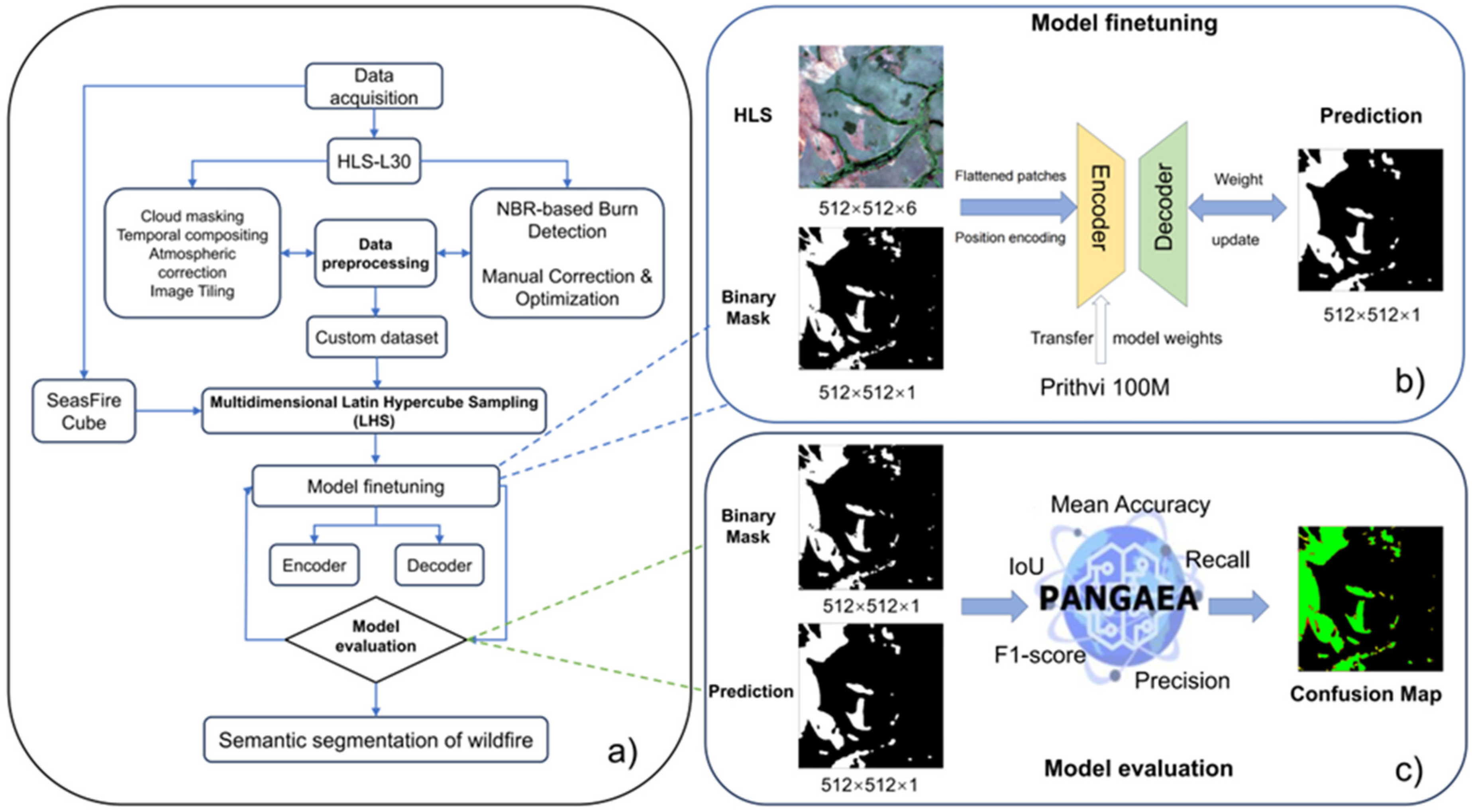
To provide a clear logical explanation of our methodology, we first outline the overall technical framework of this study before detailing the specific datasets and analytical configurations. The framework begins with data acquisition and preprocessing, where high-resolution imagery and multidimensional environmental variables are integrated and rigorously filtered. Next, a multidimensional LHS strategy is applied to build a highly representative training subset. The following step is model fine-tuning, which adapts the Prithvi EFM to the specific task of identifying small-scale burn scars. Finally, the workflow concludes with evaluation and statistical analysis, where we comprehensively assess both the model’s segmentation performance and the sampling strategy’s statistical reliability. The detailed implementation of each stage, along with the comprehensive visualization of the entire workflow, are presented in the subsequent subsections.

2.1. Study Area

The African region is the primary focus of this study. While it contributes approximately 70% of the global burned area, the fire regime in Africa is uniquely characterized by small-scale, fragmented agricultural burnings and shifting cultivation practices, rather than just large contiguous wildfires [1,33]. These fires often occur in highly heterogeneous transition zones, resulting in burn scars that are spatially scattered and spectrally subtle in nature. Effective management depends on the accurate mapping of these fragmented burns, given the ecological sensitivity of these biomes and their significant contribution to global carbon emissions [34].

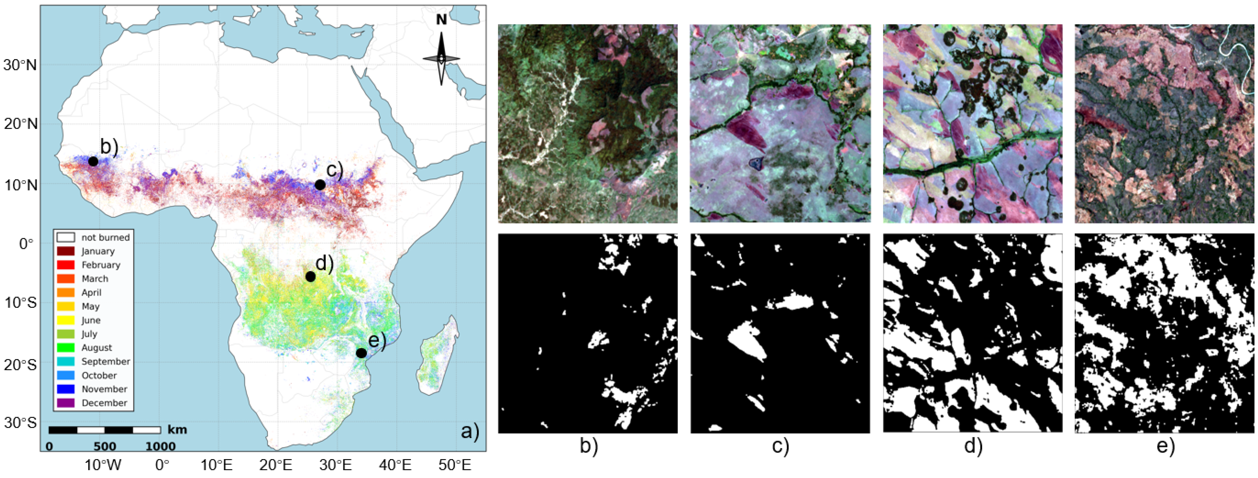
From a methodological perspective, Africa’s environmental complexity provides an ideal testing ground for data-centric strategies. As illustrated in Figure 1, this study utilized the FireCCI Small Fire Database (FireCCISFD20) [5] to map the spatiotemporal distribution of wildfires across the continent for the year 2019. This dataset was specifically selected because it was derived from high-resolution Sentinel-2 imagery (20 m), enabling the detection of small-scale burn scars that are frequently omitted by coarse-resolution global products. The visualization highlights the distinct seasonality of fire regimes, shifting from the Northern Hemisphere in the early months to the Southern Hemisphere later in the year. The selected examples (b, c, d, and e) capture this wide range of pyromes, extending from the Sahelian zone to the Miombo woodlands. This high degree of variance in both phenology and physical appearance creates a complex feature space that challenges SRS. By specifically targeting these diverse landscape characteristics and burn severities, we aimed to construct a dataset that included hard examples. This lays the necessary groundwork for the subsequent LHS strategy to ensure a robust model generalization.

2.2. Data Acquisition and Preparation

2.2.1. Satellite Imagery and Preprocessing

To capture the fine-grained spatial details of fragmented burn scars and their temporal evolution, we used HLS L30 products [6]. The HLS L30 dataset provides seamless 30 m spatial resolution with a high revisit frequency, which is critical for monitoring the rapid dynamics of vegetation fires in Africa. We acquired data covering the entire year of 2019 to encompass the full seasonal cycle of the wildfire dynamics. As illustrated in the workflow, the preprocessing pipeline was designed rigorously to ensure high-quality inputs. This included cloud masking using the Function of Mask (Fmask) algorithm [35], a robust method that leverages object-based cloud and cloud shadow matching to accurately identify atmospheric contaminants. We also applied temporal compositing to minimize residual noise and systematic image tiling to standardize the input dimensions (512 × 512 pixels) for the neural network.

2.2.2. Ground Truth Generation

A realistic and high-precision ground-truth dataset was developed using a hybrid semi-automated approach. First, we calculated the Normalized Burn Ratio (NBR) from the HLS data to generate initial burn masks. As noted in recent studies [36], NBR-based thresholding provides a solid starting point for identifying burned areas. However, automated methods often confuse burn scars with water bodies, cloud shadows and dark soils. To fix these errors and ensure accurate labels, we implemented a strict quality control mechanism like double-blind grading. Specifically, each image was manually corrected by two independent annotators. We then compared their results by calculating the Intersection over Union (IoU) score to measure agreement. If the IoU between the two annotations was high (above 0.85), the overlapping area was accepted as a valid ground truth. If the discrepancy was significant (IoU < 0.85), the sample was forwarded to a senior researcher for a final decision. This rigorous process minimized subjective errors and ensured consistency. By directly relying on the 30 m high-resolution HLS imagery rather than coarse-resolution automated products, this manual validation guarantees the reliability of the ground truth. It effectively captures the highly irregular boundaries, spectral complexity, and spatial heterogeneity inherent to small wildfires. The final dataset consisted of 1000 high-quality image-label pairs covering various burn severities and landscape types to serve as a reliable benchmark for model training.

2.2.3. Environmental Variables for Sampling Strategy

To construct a representative feature space for the subsequent sampling strategy, we integrated multidimensional environmental drivers from the SeasFire dataset [31], which aggregates data from sources such as ERA5 reanalysis and MODIS. We selected 31 distinct variables that were categorized into three physical groups: Meteorological conditions (e.g., Temperature, Vapor Pressure Deficit), Vegetation status (e.g., NDVI, Leaf Area Index), and Anthropogenic factors (e.g., Population Density). These variables were chosen because they fundamentally govern the fire ignition and spread probabilities. To ensure full methodological transparency, the complete list of these 31 variables, along with their units, is detailed in

Table 1. Complete list of the 31 multidimensional environmental variables used for LHS. Variables with numerical suffixes represent multi-layered or multi-class data extracted from the SeasFire dataset. Specifically, swvl1–4 denote volumetric soil water at four distinct depth layers defined by the ERA5 land surface model (0–7 cm, 7–28 cm, 28–100 cm, and 100–289 cm), which capture both immediate surface dryness and long-term subsurface drought. lccs_class_1–8 represent the fractional coverage of eight specific land cover classes within a grid cell: (1) Agriculture, (2) Forest, (3) Grassland, (4) Wetlands, (5) Settlement, (6) Shrubland, (7) Sparse vegetation, bare areas, permanent snow and ice, and (8) Water Bodies.

Full Name	DataArray Name	Unit
Vapor Pressure Deficit	vpd	hPa
Skin temperature	skt	K
Surface net solar radiation	ssr	MJ m−2
Surface Solar Radiation Downwards	ssrd	MJ m−2
Volumetric Soil Water Layer 1–4	swvl1, swvl2, swvl3, swvl4	m3/m3
Land Surface Temperature Day	lst_day	K
10 m Wind Speed	ws10	m s−1
Total Precipitation	tp	m
2 m Temperature (Max, Min, Mean)	t2m_max, t2m_min, t2m_mean	K
Mean Sea Level Pressure	mslp	Pa
Relative Humidity	rel_hum	%
Leaf Area Index	lai	m2/m2
Normalized Difference Vegetation Index	ndvi	Dimensionless
Land Cover Class 1–8	lccs_class_1 to lccs_class_8	%
Drought Code (Max, Mean)	drought_code_max, drought_code_mean	Dimensionless
Fire Weather Index (Max, Mean)	fwi_max, fwi_mean	Dimensionless
Population Density	pop_dens	persons/km2

.

Our variable selection focused on these dynamic drivers because they fundamentally govern pre-fire fuel accumulation, burn severity, and the resulting post-fire spectral signatures. For instance, Skin Temperature was specifically selected alongside 2 m air temperature because it directly reflects the radiative thermal state of the land surface. It is highly sensitive to canopy moisture stress and fuel dryness, making it a critical indicator of burn intensity. Conversely, static topographic and geomorphological characteristics (e.g., elevation, slope) were not explicitly included in the LHS feature space. While topography significantly influences active fire spread behavior, the post-fire spectral appearance and segmentation boundaries in optical imagery are predominantly governed by the burned vegetation type and weather-driven fire severity, which are already comprehensively captured by our selected variables. Unlike using geographic coordinates alone, leveraging these biophysical variables allows us to characterize the environmental heterogeneity of the study area, providing the necessary high-dimensional input for the LHS method.

2.3. Multidimensional LHS Strategy

To mitigate the challenges posed by spatial autocorrelation and the long-tail distribution inherent in wildfire events, we implemented a physics-informed sampling strategy known as Multidimensional LHS. Unlike SRS, which typically operates in geographic coordinates and frequently oversamples dominant background classes, LHS operates directly within the environmental feature space. We constructed a 31-dimensional hypercube using environmental variables derived from the SeasFire dataset, as defined in Section 2.2.3. The range of each variable, such as Vapor Pressure Deficit, NDVI, and Skin Temperature, was divided into N equiprobable intervals, where N represents the target sample size. The algorithm selects sample locations to ensure that exactly one sample is drawn from each interval of every dimension [37].

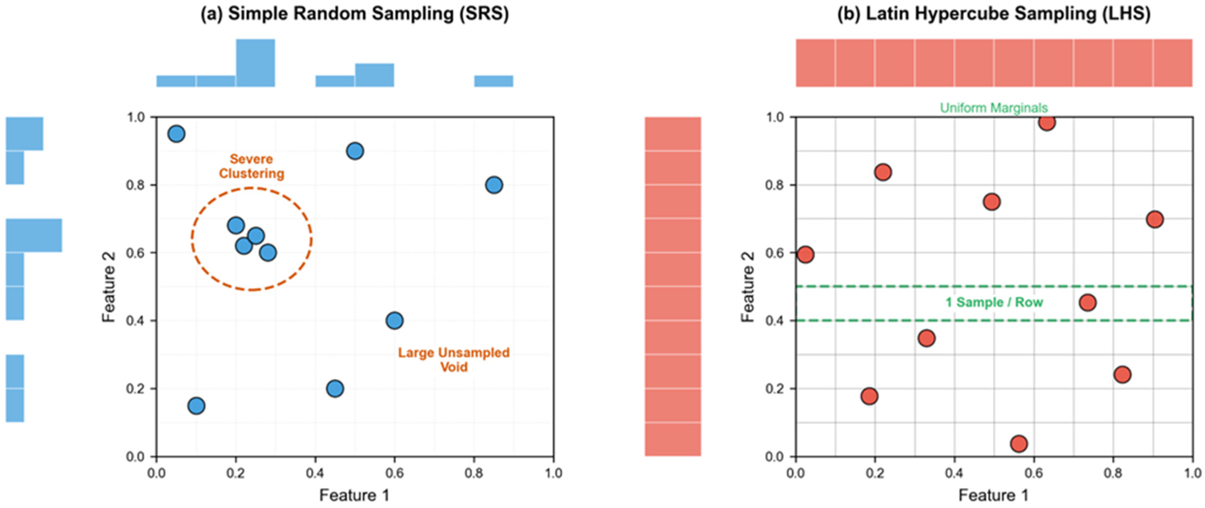
The theoretical advantage of this approach is explicitly visualized in Figure 2, which contrasts the efficacy of SRS against LHS within a normalized feature space. As shown in Figure 2a, SRS suffers from stochastic volatility, as evidenced by severe clustering (circled in orange) and large unsampled voids. Crucially, the jagged marginal histograms (blue bars) confirm that SRS fails to cover the feature space uniformly, leaving significant gaps in the data representation. In the context of geospatial fine-tuning, such clustering can cause the model to overfit specific local geomorphologies while failing to learn the global features. Conversely, Figure 2b demonstrates how LHS functions as a near-orthogonal design-of-experiments technique. The flat, uniform marginal histograms (red bars) visually confirm that every interval of the feature distribution is represented equally. Furthermore, the green dashed lines highlight the “1 Sample/Row” constraint, ensuring a maximally stratified distribution across the entire multidimensional feature space.

Crucially, this strategy ensures that the model is not merely trained under average conditions but is explicitly forced to learn from hard examples located at the boundaries of the ecological envelope. These include fires occurring under extremely humid conditions, low-biomass deserts, or complex urban-wildland interfaces. By capturing these edge cases and rare geophysical phenomena, the LHS minimizes redundancy and maximizes the information content per sample. For the fine-tuning of large-scale models on petabyte-scale satellite imagery, this approach yields more stable gradient updates and achieves the target accuracy with significantly fewer samples. Consequently, it reduces both the computational cost and carbon footprint of the training process [27].

2.4. Model Architecture and Fine-Tuning Verification

2.4.1. Foundation Model Backbone

In this study, we proposed a specialized semantic segmentation framework for wildfire burn scars, constructed by optimizing the Prithvi 100 M EFM as an encoder backbone and integrating it with a hierarchical decoding strategy. Prithvi 100 M represents a paradigm shift in Earth observation AI, built on a scalable ViT architecture [20]. Unlike traditional CNNs that rely on local receptive fields, Prithvi utilizes self-attention mechanisms to capture long-range dependencies and global contextual information, which are critical for identifying large-scale environmental patterns across diverse landscapes. The model was pre-trained using a MAE objective [19] on the massive HLS dataset. This SSL strategy compels the model to reconstruct random masked patches of multispectral imagery, thereby learning robust and spectrally aware feature representations without the need for labeled data [17].

2.4.2. Hierarchical Decoding and Fine-Tuning

The fine-tuning process, as illustrated in Figure 3b, adopts a sophisticated transfer-learning paradigm. The workflow begins with processing HLS imagery (tensor shape 512 × 512 × 6) into flattened patches, which are then embedded with positional information and fed into the encoder. Instead of using the final output of the transformer, we implemented a hierarchical feature aggregation strategy. We extracted multilevel feature maps from the intermediate layers of the transformer (indices 3, 5, 7, and 11). This design allows the model to simultaneously leverage low-level spatial details (from shallow layers) for precise boundary delineation and high-level semantic contexts (from deep layers) for object categorization to achieve accurate segmentation. These hierarchical features are fused using a Unified Perceptual Parsing Network (UPerNet) decoder [38]. The UPerNet architecture incorporates a Pyramid Pooling Module to aggregate the global context and a Feature Pyramid Network to unify the multi-scale features. This configuration is particularly effective for wildfire segmentation because it ensures scale invariance, enabling the accurate detection of both extensive burn scars and small, fragmented fire spots.

2.4.3. Evaluation Protocol

To ensure a rigorous and reproducible assessment, model evaluation was performed using the PANGAEA benchmarking suite [32]. As shown in Figure 3c, the evaluation phase transcends the simple accuracy metrics. By aligning with PANGAEA’s standardized protocols, we computed a comprehensive set of metrics, including Mean Accuracy, IoU, Recall, F1-score, and Precision. These metrics provide a holistic view of the model’s performance, particularly in handling class imbalance. Furthermore, the generation of Confusion Maps serves as a critical diagnostic tool. By visualizing pixel-wise classification errors (distinguishing between True Positives, False Positives, and False Negatives), we can qualitatively analyze the robustness of the model in complex transition zones, such as distinguishing fresh burn scars from dark soils or water bodies.

2.5. Baseline Models for Comparative Analysis

To rigorously evaluate the efficacy of our fine-tuned Prithvi 100 M framework, we conducted a comparative analysis with five SOTA foundation models. To ensure fairness, all baseline models were fine-tuned on the same dataset using identical computational resources and evaluated using standardized PANGAEA benchmark protocols.

We first examined models that focused on spatial and geometric representations. ViT was included for its global context capabilities via self-attention [20]. However, as it was originally designed for RGB imagery, ViT lacks the inherent capacity to process non-visible spectral bands (e.g., SWIR), which are critical for burn scar discrimination. To address spatial heterogeneity, we selected Scale-MAE, the SOTA in multi-scale representation learning [39]. While Scale-MAE excels in geometric invariance through Ground Sample Distance encoding, this focus often compromises spectral depth, reducing its sensitivity in distinguishing spectrally similar classes, such as old burn scars and dark soils.

Regarding spectral adaptability and multimodal fusion, we evaluated the Dynamic Optical Foundation Model (DOFA) and CROMA. DOFA employs a wavelength-adaptive mechanism to generate dynamic weights for different sensors [40]. Although flexible, its generalized approach fails to capture the granular feature representations of the HLS dataset as effectively as a domain-specific model. Similarly, CROMA is designed to fuse radar and optical data [41]. Although powerful for structural analysis, its cross-modal architecture introduces redundancy for our purely optical task, diverting the model capacity to unnecessary radar feature alignment.

Finally, to explore semantic understanding, we selected RemoteCLIP, a vision–language foundation model [42]. Although RemoteCLIP excels in high-level concept retrieval through text–image alignment, this capability is often misaligned with the requirements of dense prediction tasks. Semantic segmentation requires pixel-level precision for boundary delineation, an area where reconstruction-based models typically outperform alignment-based models.

In conclusion, while these baselines exhibit exceptional strengths in their respective niches, Prithvi 100 M offers the most balanced solution for wildfire segmentation. Its superiority stems from two core factors: first, its MAE objective forces the model to reconstruct pixel-level details, which is intrinsically better suited for dense segmentation than contrastive learning approaches; second, its native pre-training on HLS data ensures optimal alignment with the specific spectral characteristics of the target wildfire dataset.

2.6. Experimental Design

To systematically evaluate the methodologies detailed in the preceding sections and to ensure a logical transition to our findings, we established a structured experimental framework. This framework was designed to validate the statistical reliability of the Multidimensional LHS approach, measure the data efficiency of the fine-tuned Prithvi 100 M foundation model, and benchmark its segmentation accuracy against current SOTA methods. All computational experiments were conducted under identical hardware configurations to guarantee fair and reproducible comparisons.

The first phase of the experimental design focused on validating the statistical fidelity of the proposed sampling strategy. Before analyzing any image segmentation outputs, we applied the two-sample KS test across all 31 environmental variables, which encompass meteorological conditions, vegetation status, and other factors. This step was necessary to quantitatively confirm that the selected sample subset accurately mirrored the global environmental distribution without introducing the sampling bias typically associated with SRS.

Following the statistical validation, the second phase comprised a rigorous ablation study aimed at isolating the impacts of training data volume and sampling methodology. We sequentially trained the model using datasets comprising 100, 500, and 1000 image pairs to evaluate its few-shot learning capabilities and overall scalability. Concurrently, we compared the segmentation performance and training stability of models trained via our proposed sampling strategy against those trained using conventional random sampling under identical data constraints. This evaluation relied on specific metrics including Mean Accuracy, IoU, Recall, Precision, and F1-score to capture the detailed performance variations.

The final phase of the experiment was designed to benchmark the fine-tuned Prithvi 100 M model against 5 mainstream foundation models, specifically ViT, Scale-MAE, DOFA, CROMA, and RemoteCLIP. By employing the standardized evaluation metrics mentioned above and generating pixel-level error maps, we assessed the capacity of each architecture to delineate fragmented burn scars and manage severe class imbalances. This comprehensive testing sequence directly establishes the foundation for the performance analysis detailed in the subsequent Section 3.

2.7. Evaluation Metrics

Semantic segmentation models in remote sensing applications depend on rigorous evaluation using suitable metrics to precisely define land cover and boundary objects. In this study, following the standardized protocols of the PANGAEA benchmark [32], we employed a comprehensive set of metrics to assess the model performance from multiple dimensions.

Overall Accuracy provides a worldwide perspective of the properly categorized pixels for general model performance. However, in wildfire detection tasks characterized by severe class imbalance, accuracy alone can be misleading. The IoU is especially helpful for tasks requiring exact object localization and boundary delineation of irregular burn scars [43,44]. This statistic provides a complete picture of the object segmentation quality by quantifying the spatial overlap between the predicted mask and ground truth.

To further diagnose the model’s behavior regarding false positives and false negatives, we computed the Precision, Recall, and the F1-score. Recall is critical for environmental monitoring because it measures the ability to identify all fire-affected areas, whereas precision ensures the reliability of detection by minimizing false alarms. The F1-score offers a balanced assessment that guides decisions in post-disaster resource management. The metrics were calculated as follows:

$$\mathrm{A}\mathrm{c}\mathrm{c}\mathrm{u}\mathrm{r}\mathrm{a}\mathrm{c}\mathrm{y}={\displaystyle \frac{\mathrm{T}\mathrm{P}+\mathrm{T}\mathrm{N}}{\mathrm{T}\mathrm{P}+\mathrm{T}\mathrm{N}+\mathrm{F}\mathrm{P}+\mathrm{F}\mathrm{N}}}$$

(1)

$$\mathrm{P}\mathrm{r}\mathrm{e}\mathrm{c}\mathrm{i}\mathrm{s}\mathrm{i}\mathrm{o}\mathrm{n}={\displaystyle \frac{\mathrm{T}\mathrm{P}}{\mathrm{T}\mathrm{P}+\mathrm{F}\mathrm{P}}}$$

(2)

$$\mathrm{R}\mathrm{e}\mathrm{c}\mathrm{a}\mathrm{l}\mathrm{l}={\displaystyle \frac{\mathrm{T}\mathrm{P}}{\mathrm{T}\mathrm{P}+\mathrm{F}\mathrm{N}}}$$

(3)

$$\mathrm{F}1-\mathrm{s}\mathrm{c}\mathrm{o}\mathrm{r}\mathrm{e}=2\times {\displaystyle \frac{\mathrm{P}\mathrm{r}\mathrm{e}\mathrm{c}\mathrm{i}\mathrm{s}\mathrm{i}\mathrm{o}\mathrm{n}\times \mathrm{R}\mathrm{e}\mathrm{c}\mathrm{a}\mathrm{l}\mathrm{l}}{\mathrm{P}\mathrm{r}\mathrm{e}\mathrm{c}\mathrm{i}\mathrm{s}\mathrm{i}\mathrm{o}\mathrm{n}+\mathrm{R}\mathrm{e}\mathrm{c}\mathrm{a}\mathrm{l}\mathrm{l}}}$$

(4)

$$\mathrm{I}\mathrm{o}\mathrm{U}={\displaystyle \frac{\mathrm{T}\mathrm{P}}{\mathrm{T}\mathrm{P}+\mathrm{F}\mathrm{P}+\mathrm{F}\mathrm{N}}}$$

(5)

While the previous metrics evaluate the spatial segmentation performance of the model, it is equally important to assess the statistical reliability of our sampling strategy. To quantitatively verify whether the sampled subsets accurately represent the global dataset without introducing bias, we used the two-sample KS test. As a standard non-parametric method, the KS test compares the probability distributions of two independent samples without assuming any specific prior distribution. In this study, the null hypothesis states that the multidimensional environmental variables in the sampled subset and those in the original global dataset come from the exact same continuous distribution. The test calculates the KS statistic, denoted as $D$, which measures the maximum absolute distance between the empirical cumulative distribution functions of the two datasets. A lower $D$ value indicates a higher degree of similarity. Additionally, the test provides a $p$-value that is compared against a predefined significance level, $\alpha$. By setting $\alpha =0.05$, we establish a clear threshold to determine whether any observed differences between the sampled subset and the global dataset are statistically meaningful or simply due to random chance. If the calculated $p$-value is greater than this threshold ($p>0.05$), it means there is no statistically significant difference between the two distributions. Therefore, a low $D$ statistic combined with a $p$-value greater than 0.05 provides strong evidence that our LHS strategy successfully preserves the global multidimensional feature space without introducing sampling bias. This ensures that the model is trained on a truly representative dataset.

3. Results

3.1. Validation of the Multidimensional LHS Strategy

The credibility of the segmentation performance reported in the previous sections is fundamentally underpinned by the high quality of the validation dataset constructed via our proposed Multidimensional LHS strategy. Unlike SRS, LHS is designed to ensure stratified and uniform coverage of the high-dimensional feature space. This section provides a rigorous validation of the proposed approach, demonstrating its superiority in preserving the statistical properties of the global population within a compact sample subset.

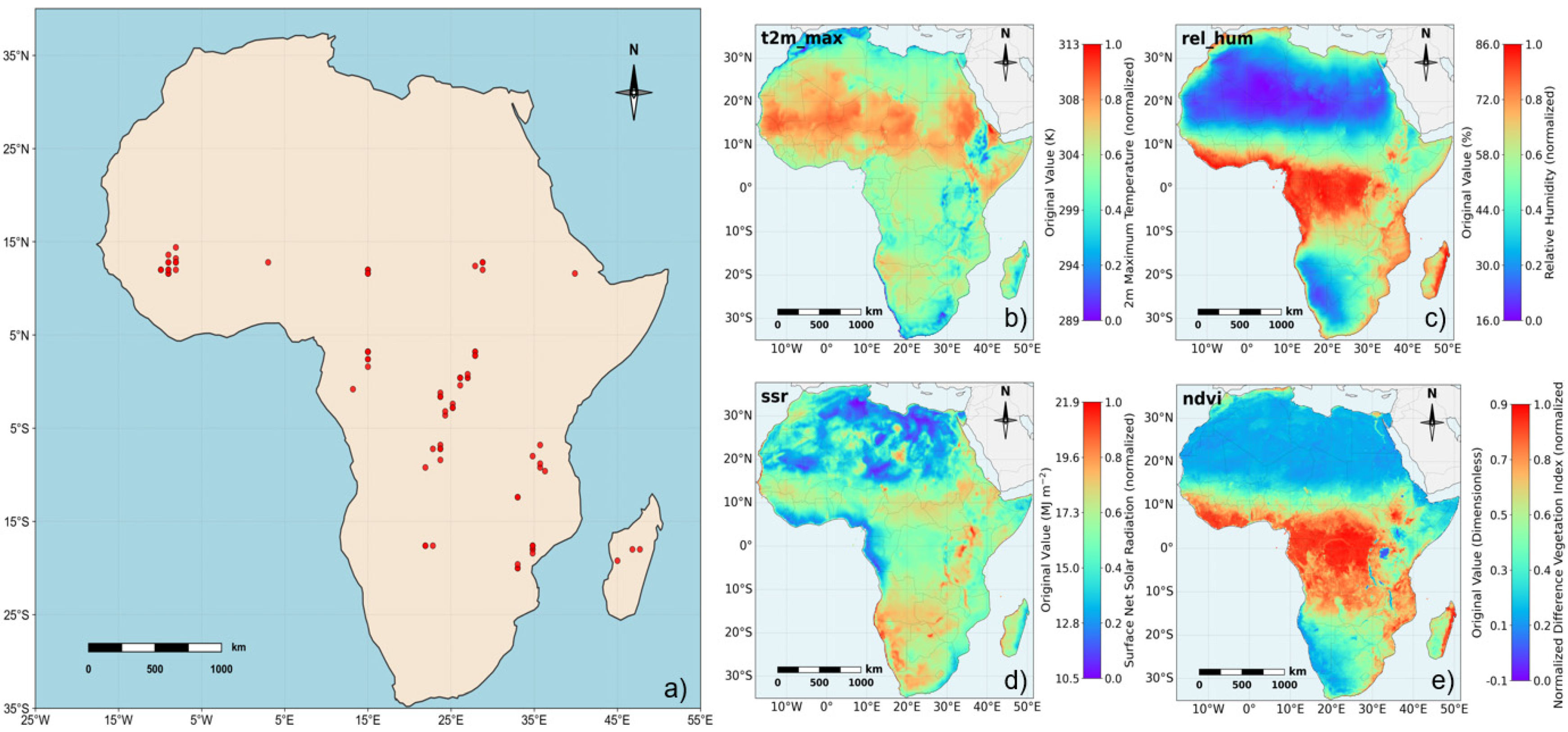
The efficacy of the sampling strategy extends beyond mere geographic coverage to a comprehensive representation of the environmental feature space. As illustrated in Figure 4, the selected sites are not only spatially dispersed but also span the critical climatic and ecological gradients that drive fire dynamics. The spatial patterns of the Maximum Temperature (Figure 4b) and Relative Humidity (Figure 4c) highlight the dataset’s inclusion of diverse thermodynamic conditions, which directly influence the fuel moisture content and ignition probabilities. Furthermore, the variation in NDVI (Figure 4e) confirmed that the sampling captured a wide spectrum of vegetation densities, ranging from sparse shrublands to dense forests. By covering these environmental extremes rather than clustering around the mean, this strategy ensures that the model is exposed to the full physics of fire regimes, including the hard examples found at the boundaries of these ecological envelopes.

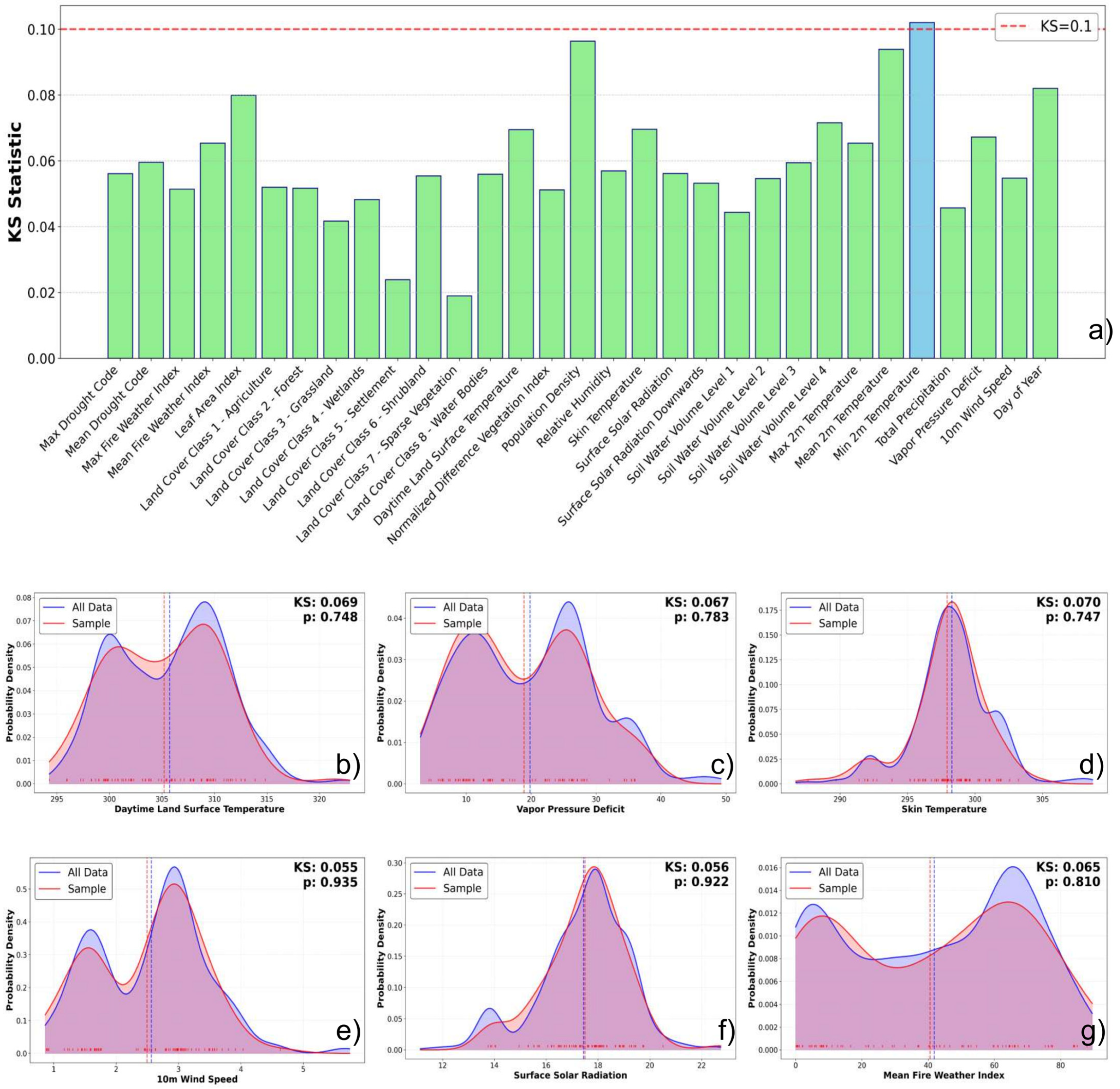
The statistical fidelity of the proposed sampling framework is rigorously quantified in Figure 5. Addressing the non-Gaussian nature of environmental variables is a critical challenge in wildfire modeling. Figure 5a demonstrates that the Multidimensional LHS strategy effectively mitigates the sampling bias. As illustrated, the KS statistics for the vast majority of variables remain well below the stringent threshold of 0.1, and the corresponding p values consistently exceed 0.05. This statistical evidence confirms that the marginal distributions of the sample are statistically identical to the global population. More importantly, the Probability Density Functions presented in Figure 5b–g reveals the ability of the method to preserve complex distributional topologies. For instance, the “10 m Wind Speed” variable in Figure 5e exhibits a distinct bimodal distribution, which is characteristic of varying atmospheric stability regimes. Unlike SRS, which often smooths such multimodal features toward a normal distribution, the LHS-derived subset (red curves) faithfully reproduces these peaks, closely tracking the global dataset (blue curves). Similarly, the method captures the skewness in the “Mean Fire Weather Index” (Figure 5g) and the leptokurtic nature of “Skin Temperature” (Figure 5d). Preserving such distributional details is fundamental for training robust foundation models, as it prevents the network from overfitting to the average conditions and enhances its generalization capability across heterogeneous landscapes.

Crucially, this representativeness was quantitatively validated by the computed statistical metrics shown in the subplots. The visualized variables exhibited consistently low KS distances ranging from 0.055 to 0.070, accompanied by high p-values exceeding 0.74 across all cases. Notably, the “10 m Wind Speed” variable achieved a p-value of 0.935, providing strong evidence that the null hypothesis cannot be rejected. This result supports the conclusion that the sample and global distributions are statistically identical, confirming that the stratified sampling strategy successfully captures the full dynamic range of the feature space without introducing a statistical bias.

Preserving these distributional details is fundamental for training robust foundation models. The core principle is that matching the training data distribution with real-world environments minimizes data mismatch during the learning process. By ensuring the model learns from the full variety of environmental conditions, including the extreme values shown in the tails of the probability density curves, the network avoids overfitting to average situations. In practice, capturing the bimodal wind speed allows the model to accurately identify both highly directional burn scars caused by strong winds and more circular scars formed under calm weather. Additionally, keeping the skewed distribution of the Fire Weather Index helps the model detect the subtle visual signs of low-intensity fires, rather than only finding severe burns. This complete training exposure builds a more accurate decision boundary, which directly leads to the higher mIoU and the significant drop in omission errors seen in our results. Therefore, this statistical matching is the main reason the model achieves better boundary accuracy and stronger generalization across different African landscapes.

3.2. Ablation Study

The ablation analysis reveals the individual contributions of the dataset size and sampling strategy to the overall model performance. These results verify the data efficiency of the fine-tuned Prithvi foundation model and highlight the specific advantages of the proposed Multidimensional LHS method.

3.2.1. Impact of Sample Size

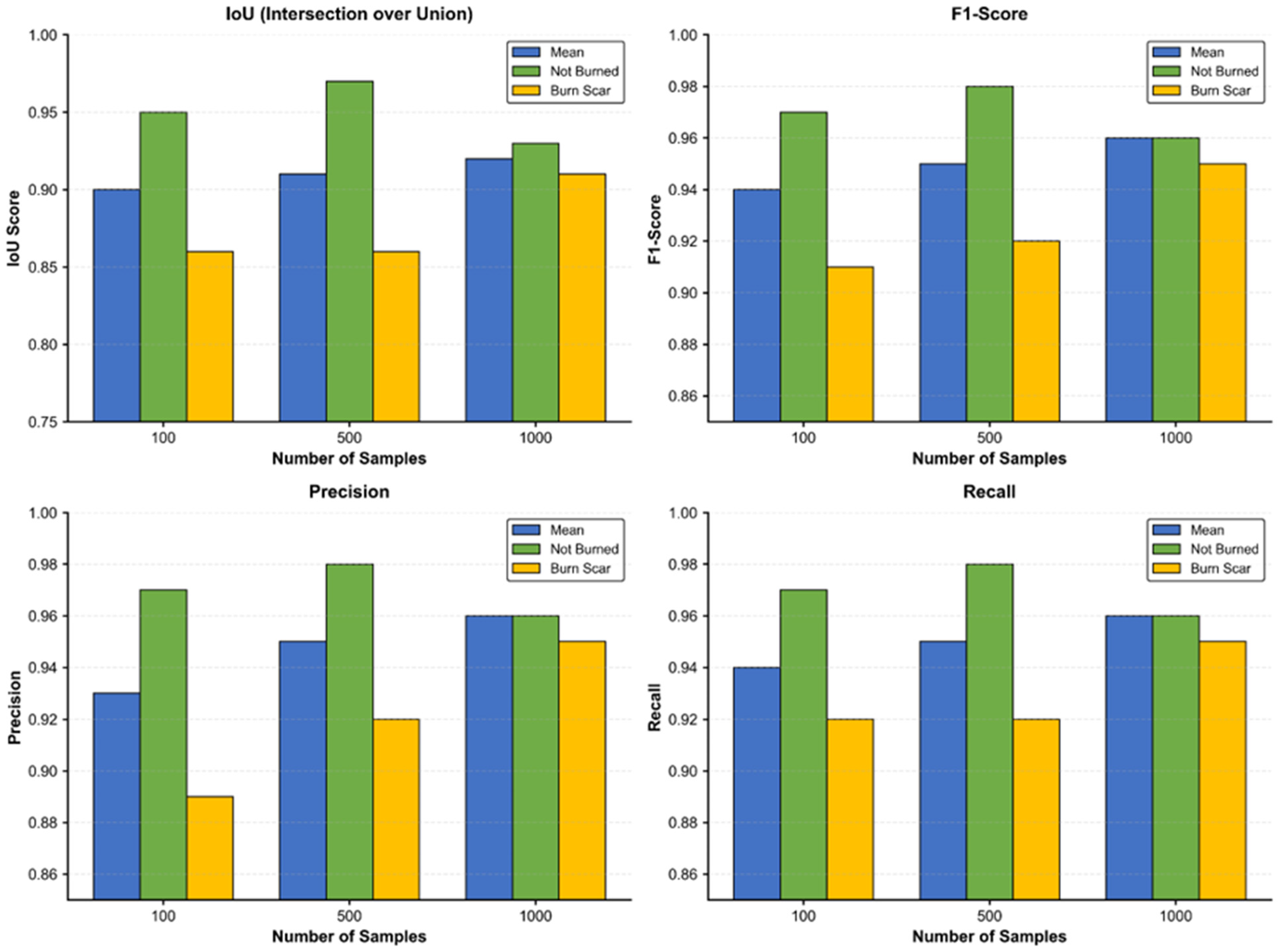
The model’s sensitivity to the training data volume across 100, 500, and 1000 sample pairs, as detailed in

Table 2. Quantitative performance metrics (IoU, F1-score, Precision, Recall, Mean Accuracy) were evaluated at different sizes (100, 500, and 1000). The values represent the mean ± standard deviation across multiple experimental runs, demonstrating both the high baseline performance at 100 samples and the improved stability at 1000 samples.

Evaluation Metrics		Number of Samples
		100	500	1000
IoU	mean	0.90 ± 0.0006	0.91 ± 0.0004	0.92 ± 0.0003
	Not burned	0.95 ± 0.0005	0.97 ± 0.0005	0.93 ± 0.0004
	Burn scar	0.86 ± 0.0007	0.86 ± 0.0006	0.91 ± 0.0005
F1-score	mean	0.94 ± 0.0005	0.95 ± 0.0004	0.96 ± 0.0002
	Not burned	0.97 ± 0.0007	0.98 ± 0.0005	0.96 ± 0.0004
	Burn scar	0.91 ± 0.0006	0.92 ± 0.0005	0.95 ± 0.0003
Precision	mean	0.93 ± 0.0007	0.95 ± 0.0006	0.96 ± 0.0004
	Not burned	0.97 ± 0.0005	0.98 ± 0.0005	0.96 ± 0.0002
	Burn scar	0.89 ± 0.0008	0.92 ± 0.0006	0.95 ± 0.0005
Recall	mean	0.94 ± 0.0006	0.95 ± 0.0006	0.96 ± 0.0004
	Not burned	0.97 ± 0.0005	0.98 ± 0.0004	0.96 ± 0.0003
	Burn scar	0.92 ± 0.0008	0.92 ± 0.0007	0.95 ± 0.0004
Mean Accuracy		0.96 ± 0.0005	0.97 ± 0.0005	0.96 ± 0.0003

and visualized in Figure 6, reveals a dual advantage of robust few-shot learning capabilities and significant performance scalability.

Remarkably, even with a minimal dataset of 100 samples, the model demonstrated exceptional data efficiency. It achieved a Mean Accuracy of 0.96 and a Burn Scar IoU of 0.86. This high baseline suggests that the pretrained foundation model effectively leverages learned priors to generalize from sparse supervision, validating its potential for rapid deployment in data-scarce scenarios. However, increasing the sample size yields critical refinements in the segmentation precision. As the dataset expanded to 1000 samples, we observed a monotonic improvement across all metrics. Notably, the Burn Scar IoU surged to 0.91, and the F1-score reached 0.95. The narrowing standard deviations in Table 2 further indicate that larger datasets not only boost accuracy but also enhance the stochastic stability of the training process.

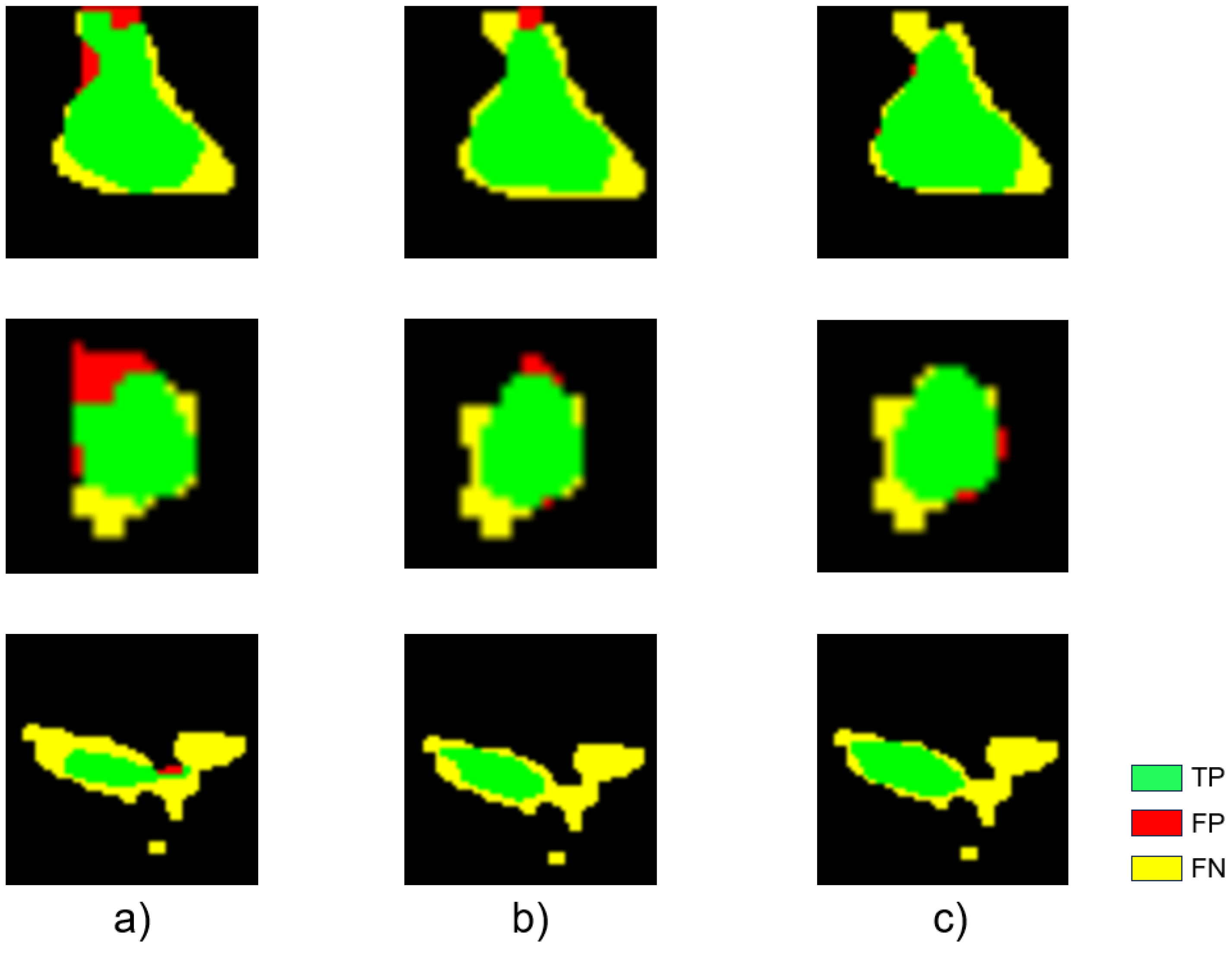
This quantitative trajectory is visually corroborated in Figure 7. At a sample size of 100 shown in Figure 7a, although the primary burn areas were correctly identified, the outputs exhibited minor fragmentation and boundary noise, indicated by red and yellow pixels. Conversely, the model trained on 1000 samples in Figure 7c produced highly coherent masks with smooth boundaries that aligned precisely with the ground truth. This confirms that, while the model is inherently few-shot capable, a sufficient volume of high-quality data remains essential for resolving complex boundary details and eliminating false positives.

3.2.2. Impact of Sampling Strategy

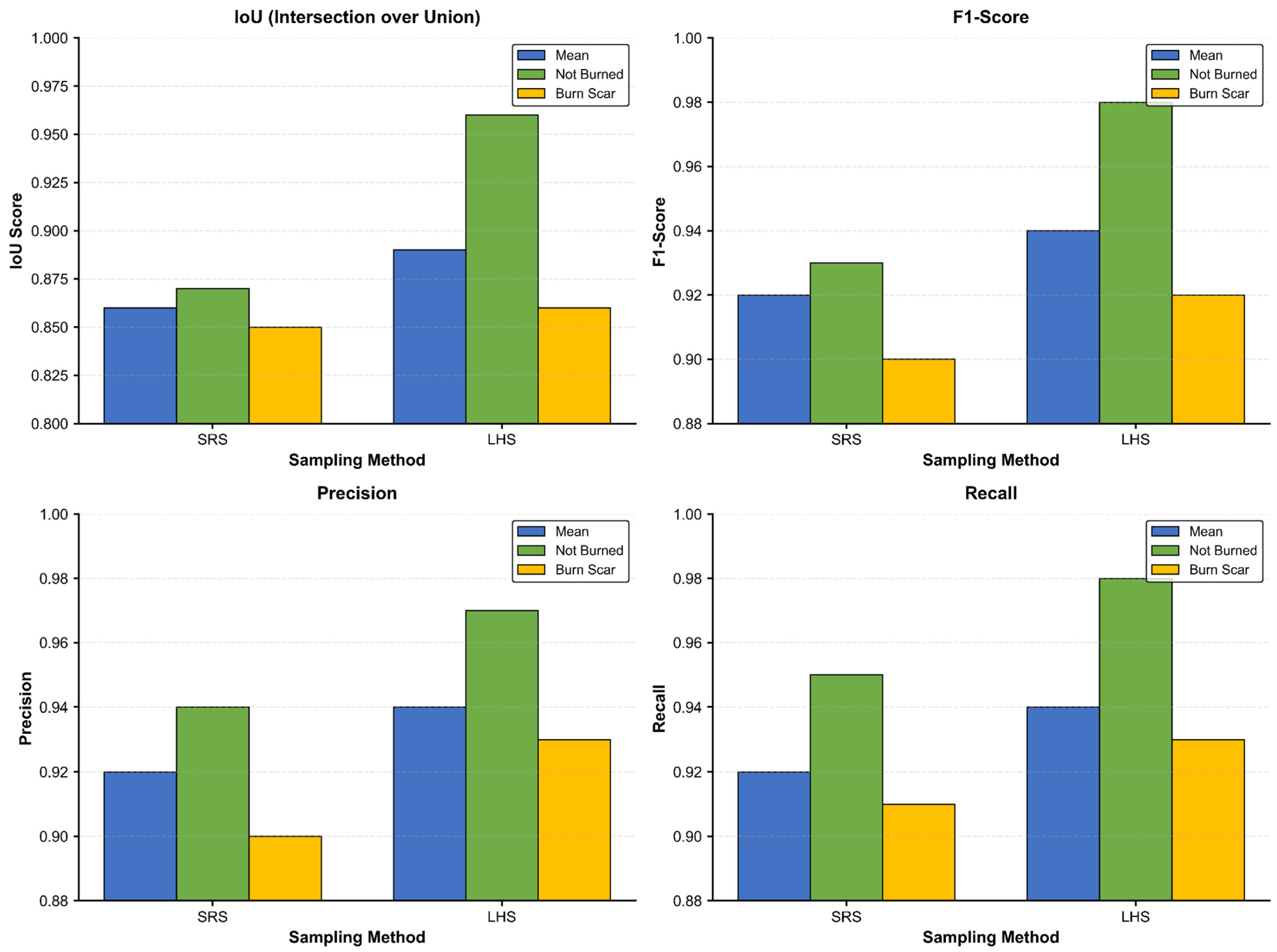
The comparison between the Multidimensional LHS strategy and conventional SRS, as shown in

Table 3. Comparative ablation study of segmentation performance using SRS and the proposed LHS strategy. The values are presented as mean ± standard deviation, indicating that LHS achieves both higher accuracy and better stability.

Evaluation Metrics		Sampling Method
		SRS	LHS
IoU	mean	0.86 ± 0.0015	0.89 ± 0.0007
	Not burned	0.87 ± 0.0013	0.96 ± 0.0005
	Burn scar	0.85 ± 0.0018	0.86 ± 0.0006
F1-score	mean	0.92 ± 0.0014	0.94 ± 0.0004
	Not burned	0.93 ± 0.0011	0.98 ± 0.0006
	Burn scar	0.90 ± 0.0017	0.92 ± 0.0004
Precision	mean	0.92 ± 0.0013	0.94 ± 0.0006
	Not burned	0.94 ± 0.0010	0.97 ± 0.0005
	Burn scar	0.90 ± 0.0016	0.93 ± 0.0007
Recall	mean	0.92 ± 0.0015	0.94 ± 0.0005
	Not burned	0.95 ± 0.0012	0.98 ± 0.0008
	Burn scar	0.91 ± 0.0019	0.93 ± 0.0006
Mean Accuracy		0.92 ± 0.0009	0.96 ± 0.0005

and Figure 8, indicates that the LHS strategy offers a dual advantage: it improves segmentation performance and enhances training stability.

First, regarding the performance accuracy, LHS consistently achieved higher scores across all metrics. As detailed in Table 3, the mIoU increased from 0.86 (SRS) to 0.89 (LHS). This improvement was particularly noticeable in the “Burn Scar” class, where the Recall rate increased from 0.91 to 0.93. This suggests that the model can identify fire perimeters more effectively when trained with LHS-sampled data. Second, regarding model stability, LHS demonstrated a significantly lower variance between different experimental runs. The standard deviation values in Table 3 are consistently smaller for LHS than for SRS, with the Burn Scar Recall standard deviation dropping from 0.0019 to 0.0006. This indicates that LHS reduces randomness in the training process, leading to more reliable and reproducible results.

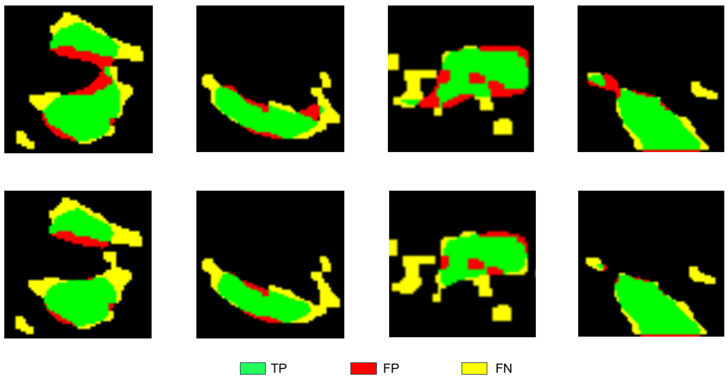
These quantitative improvements are visually confirmed in Figure 9. The top row shows that the model trained using SRS tends to produce scattered misclassified pixels, visible as red and yellow areas, resulting in fragmented segmentation maps. In contrast, the bottom row shows that the LHS strategy produced fewer error pixels overall, with a noticeable reduction in red false positives in the background and fewer yellow false negatives along the burn-scar edges in several examples. As a result, the predicted burn regions show fewer small breaks caused by misclassified pixels, and the main burned patches appear more consistently connected across the compared cases. This difference is likely because SRS often selects redundant data points that are close to each other, whereas LHS ensures a more uniform coverage of the data distribution, allowing the model to learn a more complete representation of the features and thus reducing these types of errors.

3.3. Assessing Model Superiority and Universality in Complex Burn Scar Detection

Our experimental study established a new SOTA for wildfire burn scar segmentation by demonstrating that fine-tuning the Prithvi 100 M model end-to-end consistently achieved outstanding performance. As reported in

Table 4. Quantitative performance comparison of the segmentation results. The table reports the IoU, F1-score, Precision, Recall, and Mean Accuracy for the Prithvi 100 M fine-tuned framework compared against mainstream foundation models (CROMA, DOFA, RemoteCLIP, Scale-MAE, and ViT). Specific metrics for the “Not burned” and “Burn scar” classes are detailed to highlight the class-wise performance differences. Values are presented as mean ± standard deviation, highlighting that Prithvi achieved not only the highest accuracy but also the highest stability among all tested models.

Evaluation Metrics		Model
		CROMA	DOFA	RemoteCLIP	Scale-MAE	ViT	Prithvi
IoU	mean	0.88 ± 0.0007	0.85 ± 0.0006	0.65 ± 0.0023	0.67 ± 0.0018	0.69 ± 0.0014	0.91 ± 0.0005
	Not burned	0.95 ± 0.0005	0.93 ± 0.0005	0.77 ± 0.0019	0.83 ± 0.0015	0.84 ± 0.0011	0.96 ± 0.0004
	Burn scar	0.82 ± 0.0010	0.77 ± 0.0009	0.50 ± 0.0029	0.51 ± 0.0024	0.54 ± 0.0019	0.87 ± 0.0007
F1-score	mean	0.94 ± 0.0006	0.91 ± 0.0005	0.77 ± 0.0021	0.79 ± 0.0017	0.81 ± 0.0013	0.95 ± 0.0005
	Not burned	0.97 ± 0.0005	0.96 ± 0.0005	0.87 ± 0.0018	0.90 ± 0.0014	0.91 ± 0.0010	0.98 ± 0.0003
	Burn scar	0.90 ± 0.0009	0.87 ± 0.0008	0.66 ± 0.0026	0.68 ± 0.0022	0.70 ± 0.0017	0.93 ± 0.0006
Precision	mean	0.93 ± 0.0008	0.91 ± 0.0007	0.82 ± 0.0025	0.80 ± 0.0020	0.81 ± 0.0015	0.94 ± 0.0006
	Not burned	0.97 ± 0.0006	0.97 ± 0.0006	0.81 ± 0.0020	0.90 ± 0.0016	0.90 ± 0.0012	0.97 ± 0.0004
	Burn scar	0.89 ± 0.0011	0.85 ± 0.0008	0.84 ± 0.0031	0.70 ± 0.0026	0.73 ± 0.0020	0.93 ± 0.0008
Recall	mean	0.94 ± 0.0007	0.92 ± 0.0007	0.75 ± 0.0024	0.78 ± 0.0019	0.80 ± 0.0014	0.95 ± 0.0005
	Not burned	0.97 ± 0.0005	0.95 ± 0.0006	0.94 ± 0.0019	0.91 ± 0.0015	0.92 ± 0.0011	0.96 ± 0.0004
	Burn scar	0.92 ± 0.0010	0.89 ± 0.0007	0.55 ± 0.0030	0.66 ± 0.0025	0.68 ± 0.0018	0.94 ± 0.0007
Mean Accuracy		0.96 ± 0.0007	0.94 ± 0.0005	0.81 ± 0.0018	0.85 ± 0.0015	0.86 ± 0.0012	0.97 ± 0.0004

, the model produced exceptional results, achieving a Mean Accuracy of 0.97 ± 0.0004 and mIoU of 0.91 ± 0.0005. Compared to the generic ViT model, this performance was remarkable. Despite sharing a similar architectural foundation, the ViT model recorded significantly lower metrics, with mIoU and Burn Scar IoU values of only 0.69 ± 0.0014 and 0.54 ± 0.0019, respectively. Furthermore, the extremely low standard deviation observed for Prithvi in Table 4 (e.g., 0.0005 for mIoU) confirms its training stability, which is superior to the high variance seen in baselines such as RemoteCLIP. This statistical robustness indicates that Prithvi is not only accurate but also highly reproducible across the experimental runs.

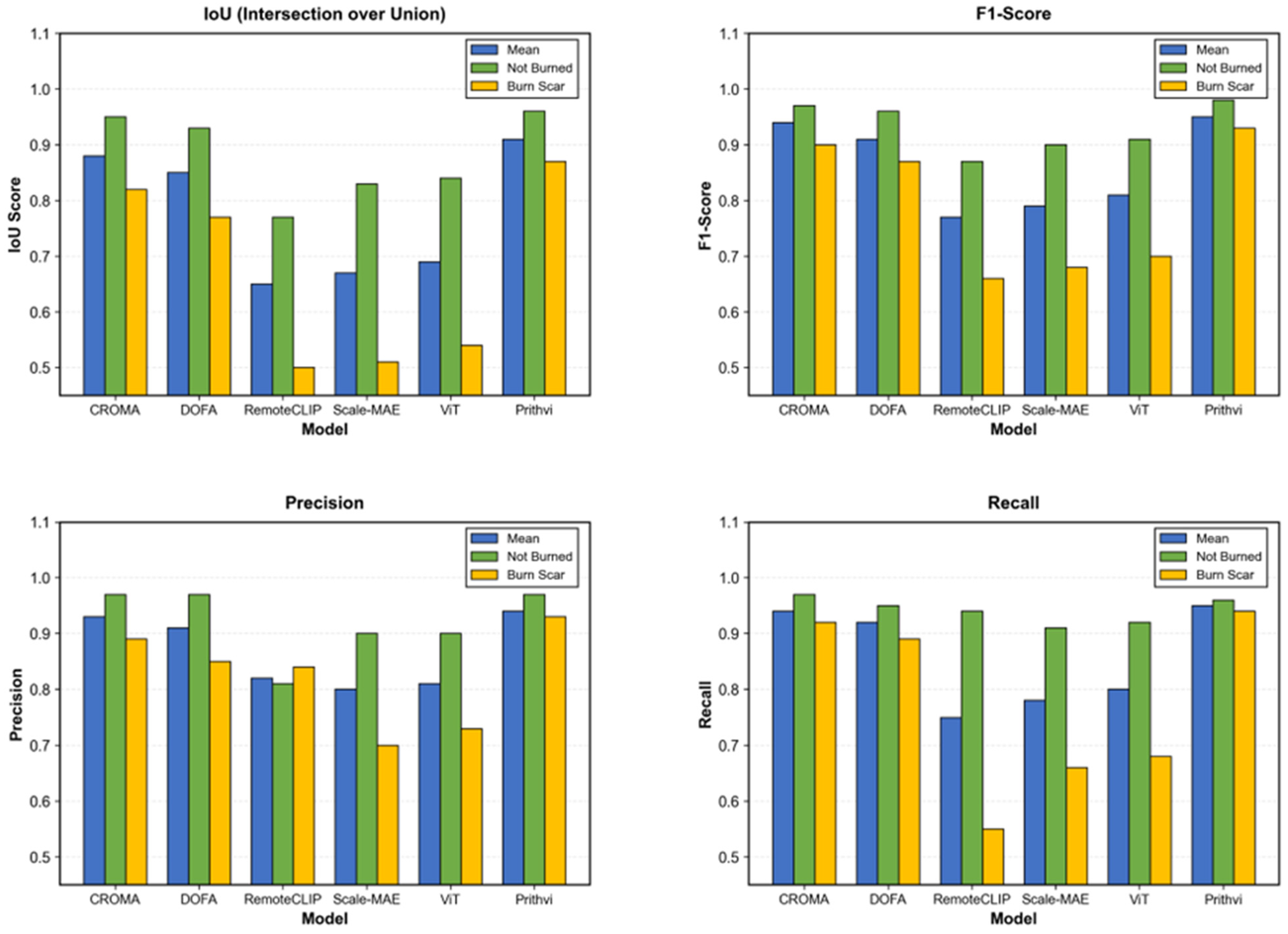
This quantitative gap is visually reinforced by the bar charts in Figure 10. Prithvi (the far-right group) dominated all four metrics (IoU, F1, Precision, Recall). The advantage is most pronounced in the challenging “Burn Scar” category (yellow bars), where Prithvi achieves an IoU of 0.87 compared to ViT’s 0.54. In contrast, the RemoteCLIP model showed a remarkable imbalance between precision and recall: while its Burn Scar Precision was decent (0.84), its Recall was critically low (0.55, as shown by the short yellow bar in the RemoteCLIP group), resulting in a mIoU of only 0.65. This discrepancy suggests that although the model is conservative in its predictions, it misses nearly half of the actual fire damage, making it less suitable for comprehensive hazard detection.

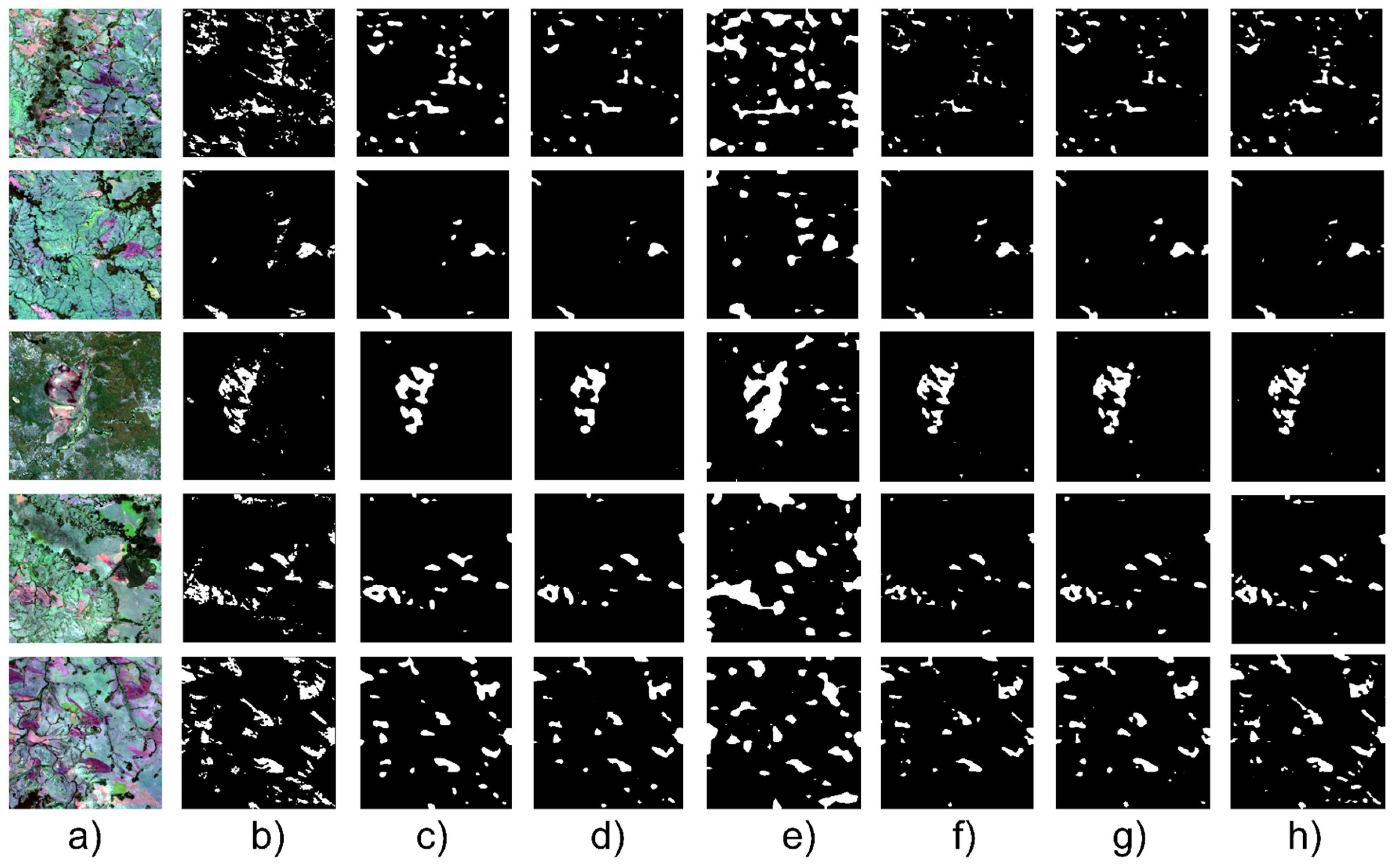
Having established the statistical advantage, Figure 11 presents convincing qualitative visual evidence of the superiority of the Prithvi framework in defining wildfire burn scars. In the difficult scenarios shown in each row, the Prithvi model (column h) consistently generated accurate and refined segmentation masks. As demonstrated by the precise delineation of scattered small burn patches in the first two rows and complex patterns in the third and fifth rows, it faithfully captured detailed scar boundaries and subtle internal unburned islands. In contrast, baseline models exhibit varying degrees of limitations. A key source of error is confusion between burn scars and other dark surfaces (e.g., shadows or dark soil), which can lead to false positives or missing regions. Scale-MAE (column f) exhibited significant noise and over-segmentation, failing to effectively distinguish unburned vegetation from burn scars. This results in many small isolated detections and fragmented masks, indicating limited spatial consistency. While CROMA (column c) and DOFA (column d) outperform weaker baselines, they still fail to match the boundary precision of Prithvi, showing minor fragmentation at the edges. These boundary breaks are more visible in transition areas where burn severity changes gradually, making the true boundary less sharp. RemoteCLIP (column e) often produces masks that are either too small (under-segmentation) or locally expanded (over-segmentation), suggesting limited suitability for fine pixel-level boundary extraction. The ViT baseline (column g) tends to generate smoother and coarser boundaries and sometimes fills small internal holes, which reduces the representation of unburned islands; this is likely related to insufficient multi-scale detail in the features. Overall, the Prithvi model (column h) produces cleaner masks with fewer isolated false positives and more accurate boundary alignment across all difficult scenarios.

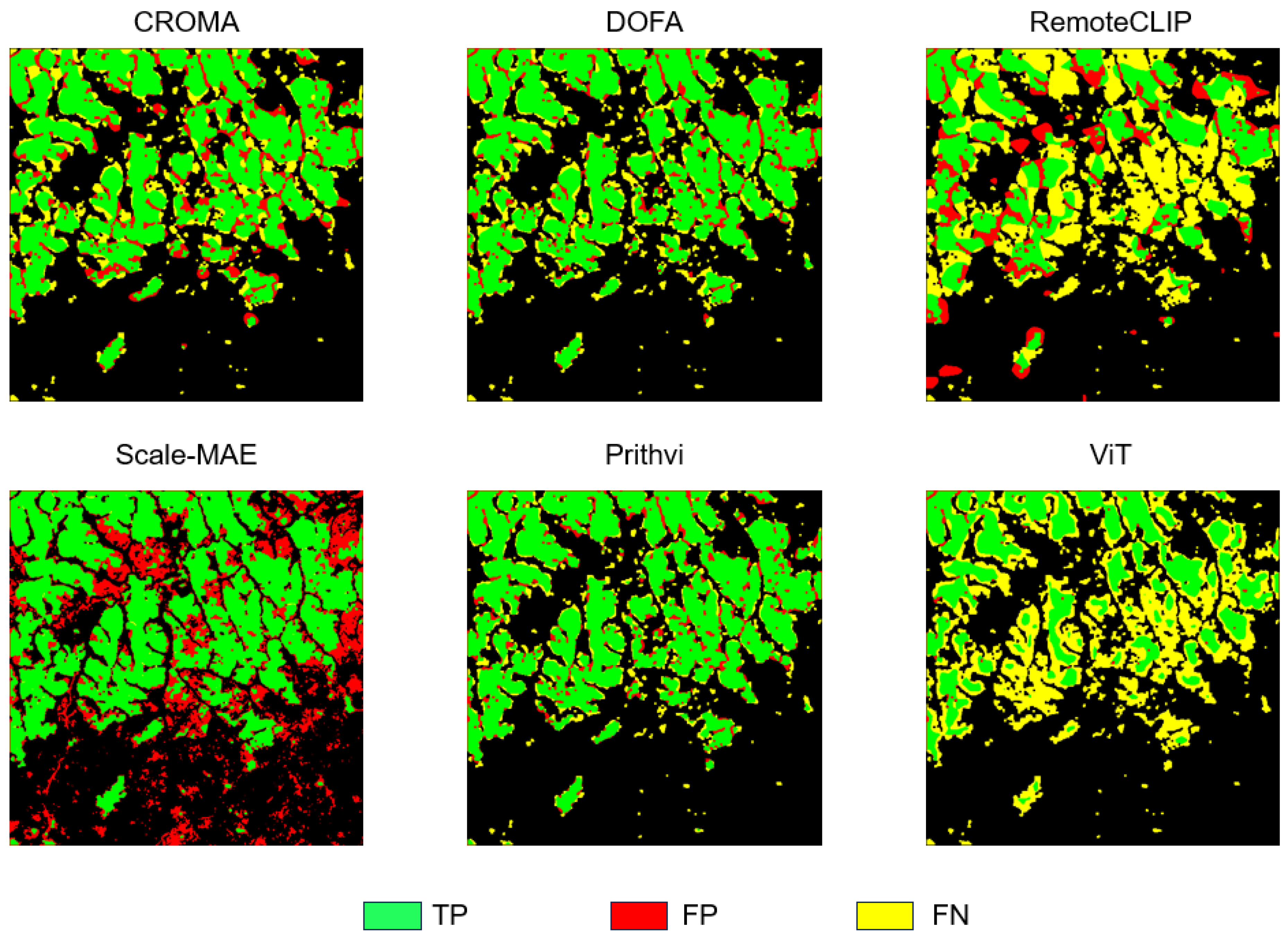
This visual superiority is corroborated by the error maps in Figure 12. Prithvi exhibited the most coherent True Positive (green) regions with negligible False Positive (red) noise or False Negative (yellow) omissions, demonstrating its precise adherence to the ground truth. In contrast, the standard ViT suffers from substantial under segmentation, characterized by extensive yellow (False Negative) areas, indicating that it missed significant portions of the burn scar. Similarly, RemoteCLIP produced large patches of misclassification (interleaved red and yellow blocks) and failed to define clear burn structures. This explicitly highlights the critical benefit of Prithvi’s domain-specific pre-training in Remote Sensing, enabling it to faithfully reconstruct difficult geographical features with minimal pixel-level errors.

In summary, this comparative analysis elucidates the synergy between the model architecture, pre-training domain, and sampling strategy. While increasing the dataset size provides statistical breadth, the specific Earth Observation pre-training of Prithvi ensures topological completeness. Consequently, the combination of the data-efficient Prithvi foundation model with the robust LHS strategy constitutes the optimal configuration, maximizing the segmentation accuracy while achieving a superior trade-off between performance and stability.

4. Discussion

The credibility of the segmentation performance reported in this study is fundamentally underpinned by the representativeness of the training data constructed using the Multidimensional LHS strategy. Our analysis indicates that the LHS method functions as a critical regularizer that shapes the decision boundary of the model more effectively than SRS. While SRS tends to oversample the mean of the distribution due to the central limit theorem, often leading to redundant data clusters [31,37], LHS enforces a stratified coverage of the high-dimensional feature space. This mechanism explains the 3.5% relative improvement in mIoU and the significant reduction in performance variance, where the standard deviation for Burn Scar Recall dropped by approximately 68% in our ablation studies. The underlying reason for this enhancement is the preservation of distributional topologies. As evidenced by the KS statistics consistently falling below 0.1, LHS successfully captured the bimodal nature of variables such as wind speed and the tail distributions of fire weather indices. By exposing the model to these complex examples at the boundaries of ecological envelopes, rather than solely the average conditions, the model learns to distinguish edge cases more effectively [45]. This capability directly translates to cleaner boundary adherence and reduced misclassification noise observed in the qualitative results, confirming that optimizing information density is more effective than merely increasing data volume [27,46].

An in-depth analysis reveals that the performance of the model is significantly influenced by environmental heterogeneity across different ecological zones in Africa. Specifically, the contribution of the Sentinel-2 red-edge bands varies across different landscapes. In arid and semi-arid savanna zones, wildfires are highly seasonal and scattered. The primary detection challenge during the dry season is distinguishing actual burn scars from naturally senescent grasses. Under these conditions, the red-edge bands are highly effective because their sensitivity to chlorophyll degradation allows the model to capture subtle spectral differences between dry vegetation and charred surfaces. Conversely, in denser and more humid woodland zones, environmental factors including canopy shadows and varying soil moisture introduce different types of spectral confusion. In these denser landscapes, the reliance on red-edge bands decreases. The model instead relies more heavily on the shortwave infrared features learned during pre-training to mitigate atmospheric interference and differentiate shadows from actual burn severity. This dynamic adaptation demonstrates that the foundation model effectively integrates spectral characteristics with underlying ecological principles, adjusting its feature extraction mechanisms based on the specific vegetation types and climate conditions of the target biome.

In addition to the sampling strategy, the substantial performance disparity between the fine-tuned Prithvi model and other baselines highlights the critical role of domain-specific pre-training over generic architectural complexity. The Prithvi model achieved a 31.9% relative improvement in mIoU compared with the standard ViT baseline. This advantage stems from Prithvi’s pre-training on multispectral HLS data, which enables the model to inherently understand the temporal and spectral signatures of burn scars, a capability that generic vision backbones trained on RGB ImageNet data do not possess [17,47,48]. Conversely, reconstruction-based architectures, such as Scale-MAE, despite their geometric invariance, underperformed with a mIoU 26.4% lower than Prithvi. This can be attributed to the objective function of the Masked Autoencoder, which focuses on global reconstruction and often smooths out the high-frequency details required for precise boundary delineation [39,49,50]. Similarly, while sophisticated models like CROMA and DOFA approached the performance of Prithvi, they still exhibited minor fragmentation at edges, likely due to the domain gap in their pre-training data [40,41,51]. Most critically, the vision–language model RemoteCLIP showed a severe limitation, with a Recall 40.8% lower than Prithvi, suggesting that text–image alignment objectives are currently insufficient for pixel-level semantic segmentation tasks, where texture and spectral nuance are paramount [42,52,53].

A significant finding of this study concerns the data efficiency of the proposed framework under few-shot conditions. Contrary to traditional deep learning paradigms that typically demand massive datasets, our fine-tuned Prithvi model achieved a competitive Burn Scar IoU of 0.86 with only 100 sample pairs, retaining 94.5% of the performance achieved with 1000 samples. This observation suggests that the EFM already possesses a rich representation of terrestrial features, and fine-tuning serves to adapt these learned priors to the specific downstream task rather than learning features from scratch [54,55,56]. This high data efficiency implies that for specialized Earth Observation tasks, the quality and diversity of samples ensured by LHS are significantly more determinant than sheer volume, offering a viable pathway for deploying models in data-scarce regions [57,58,59]. Furthermore, these ablation results regarding sample size provide practical guidance for balancing accuracy and operational cost. We recommend a tiered sampling strategy tailored to the specific needs of local industrial and forestry departments. African grassland wildfires are highly seasonal and scattered, requiring immediate attention and rapid deployment for routine monitoring. Local management authorities can achieve this by utilizing a minimal dataset of 100 optimized samples. Operating under this small-sample condition significantly reduces data annotation costs and shortens the monitoring cycle from several months to a few days. This provides an efficient tool for early warning and rapid industrial response, such as protecting agricultural and mining assets. On the other hand, tasks requiring high boundary precision, including end-of-season carbon emission accounting or post-fire ecological assessments, can utilize an expanded dataset of 1000 samples. By aligning data requirements with the seasonal characteristics of African wildfires, this methodology provides a highly adaptable and cost-effective solution, demonstrating its irreplaceable value in practical scenarios where traditional models requiring massive datasets often fail.

Despite these promising results, several limitations warrant further investigations. First, our experiments were geographically confined to Sub-Saharan Africa. While the model generalizes well within this biome, its transferability to distinct fire regimes, such as the boreal forests of Canada or the eucalyptus bushlands of Australia, remains unverified without further cross-continental testing [11]. Second, ground truth generation relied on the manual correction of HLS imagery. While rigorous, this process is inherently limited by the 30 m resolution of the source data, and incorporating very high-resolution imagery would provide a more granular benchmark for evaluating boundary precision [60]. Finally, our ablation study primarily focused on the sample size and sampling strategy. Future research should expand to investigate other hyperparameter sensitivities, such as patch size variations, masking ratios, and different fine-tuning depths, to fully optimize the adaptation of foundation models for disaster monitoring [33,61].

5. Conclusions

This study presents a systematic approach for optimizing the fine-tuning of EFMs to address the challenge of identifying small-scale burn scars in heterogeneous landscapes. By synergizing the Prithvi 100 M model with a Multidimensional LHS strategy, our framework effectively overcomes the dual constraints of spectral complexity and data scarcity that limit traditional deep learning paradigms in Sub-Saharan Africa. The experimental findings conclusively demonstrate the superiority of this optimization strategy over the existing ones. The fine-tuned Prithvi model achieved a mIoU of 0.91, representing a relative improvement of approximately 32% over the standard ViT baseline and significantly outperforming reconstruction-based methods, such as Scale-MAE. Crucially, the proposed LHS strategy proved indispensable for this performance; by ensuring the statistical representativeness of the training data (KS < 0.1), it enhanced the model’s ability to delineate the complex boundaries of small-scale burn scars, where SRS often fails. Furthermore, the framework exhibited exceptional data efficiency, retaining 94.5% of its peak performance with only 100 training samples, thereby validating the capability of foundation models to generalize from sparse supervision when the sampling strategy is optimized rigorously. Consequently, it offers an irreplaceable and highly adaptable solution for local industrial and forestry departments. By significantly shortening the monitoring cycle and reducing data costs, this framework is uniquely suited for the rapid deployment required to manage the seasonal and scattered nature of African wildfires. In conclusion, this study validates the paradigm shift towards leveraging pretrained geospatial foundation models for specialized Earth Observation tasks. By demonstrating that optimizing fine-tuning through representative sampling is as critical as the model architecture, our methodology offers a scalable and operationally viable solution for disaster monitoring. These advancements pave the way for more resilient environmental management systems capable of delivering rapid and accurate insights across global regions with limited ground truth data. Because the training selection is designed to cover a wide range of environmental conditions, the same fine-tuning protocol is expected to transfer to other regions and fuel types, including coniferous forests and shrublands, with limited additional labeling. In addition, boundary accuracy can be improved by combining this framework with higher-resolution imagery, since finer spatial detail can better separate narrow burn edges from nearby unburned surfaces. Future work will focus on testing this transfer across multiple biomes and on integrating higher-resolution inputs in a consistent way, while keeping the workflow efficient for operational use.

References

1. Ramo, R.; Roteta, E.; Bistinas, I.; van Wees, D.; Bastarrika, A.; Chuvieco, E.; van der Werf, G.R. African burned area and fire carbon emissions are strongly impacted by small fires undetected by coarse resolution satellite data. Proc. Natl. Acad. Sci. USA 2021, 118, e2011160118. [Google Scholar] [CrossRef] [Scilit]
2. Schroeder, W.; Oliva, P.; Giglio, L.; Csiszar, I.A. The New VIIRS 375m active fire detection data product: Algorithm description and initial assessment. Remote Sens. Environ. 2014, 143, 85–96. [Google Scholar] [CrossRef] [Scilit]
3. Giglio, L.; Boschetti, L.; Roy, D.P.; Humber, M.L.; Justice, C.O. The Collection 6 MODIS burned area mapping algorithm and product. Remote Sens. Environ. 2018, 217, 72–85. [Google Scholar] [CrossRef] [Scilit] [PubMed]
4. Meng, X.; Yu, Y.; Ginoux, P. Rise in dust emissions from burned landscapes primarily driven by small fires. Nat. Geosci. 2025, 18, 586–592. [Google Scholar] [CrossRef] [Scilit]
5. Roteta, E.; Bastarrika, A.; Padilla, M.; Storm, T.; Chuvieco, E. Development of a Sentinel-2 burned area algorithm: Generation of a small fire database for sub-Saharan Africa. Remote Sens. Environ. 2019, 222, 1–17. [Google Scholar] [CrossRef] [Scilit]
6. Claverie, M.; Ju, J.; Masek, J.G.; Dungan, J.L.; Vermote, E.F.; Roger, J.-C.; Skakun, S.V.; Justice, C. The Harmonized Landsat and Sentinel-2 surface reflectance data set. Remote Sens. Environ. 2018, 219, 145–161. [Google Scholar] [CrossRef] [Scilit]
7. LeCun, Y.; Bengio, Y.; Hinton, G. Deep learning. Nature 2015, 521, 436–444. [Google Scholar] [CrossRef] [Scilit]
8. LeCun, Y.; Boser, B.; Denker, J.S.; Henderson, D.; Howard, R.E.; Hubbard, W.; Jackel, L.D. Backpropagation Applied to Handwritten Zip Code Recognition. Neural Comput. 1989, 1, 541–551. [Google Scholar] [CrossRef] [Scilit]
9. Ronneberger, O.; Fischer, P.; Brox, T. U-Net: Convolutional Networks for Biomedical Image Segmentation 2015. Available online: https://arxiv.org/abs/1505.04597 (accessed on 6 April 2026).
10. Chen, L.-C.; Zhu, Y.; Papandreou, G.; Schroff, F.; Adam, H. Encoder-Decoder with Atrous Separable Convolution for Semantic Image Segmentation. In Computer Vision—ECCV 2018; Ferrari, V., Hebert, M., Sminchisescu, C., Weiss, Y., Eds.; Springer International Publishing: Cham, Switzerland, 2018; pp. 833–851. [Google Scholar]
11. Chuvieco, E.; Mouillot, F.; van der Werf, G.R.; Miguel, J.S.; Tanase, M.; Koutsias, N.; García, M.; Yebra, M.; Padilla, M.; Gitas, I.; et al. Historical background and current developments for mapping burned area from satellite Earth observation. Remote Sens. Environ. 2019, 225, 45–64. [Google Scholar] [CrossRef] [Scilit]
12. Knopp, L.; Wieland, M.; Rättich, M.; Martinis, S. A Deep Learning Approach for Burned Area Segmentation with Sentinel-2 Data. Remote Sens. 2020, 12, 2422. [Google Scholar] [CrossRef] [Scilit]
13. Roteta, E.; Bastarrika, A.; Franquesa, M.; Chuvieco, E. Landsat and Sentinel-2 Based Burned Area Mapping Tools in Google Earth Engine. Remote Sens. 2021, 13, 816. [Google Scholar] [CrossRef] [Scilit]
14. Nolde, M.; Plank, S.; Riedlinger, T. An Adaptive and Extensible System for Satellite-Based, Large Scale Burnt Area Monitoring in Near-Real Time. Remote Sens. 2020, 12, 2162. [Google Scholar] [CrossRef] [Scilit]
15. Chen, Y.; Morton, D.C.; Randerson, J.T. Remote sensing for wildfire monitoring: Insights into burned area, emissions, and fire dynamics. One Earth 2024, 7, 1022–1028. [Google Scholar] [CrossRef] [Scilit]
16. Llorens, R.; Sobrino, J.A.; Fernández, C.; Fernández-Alonso, J.M.; Vega, J.A. Soil Burn Severity Assessment Using Sentinel-2 and Radiometric Measurements. Fire 2024, 7, 487. [Google Scholar] [CrossRef] [Scilit]
17. Jakubik, J.; Roy, S.; Phillips, C.E.; Fraccaro, P.; Godwin, D.; Zadrozny, B.; Szwarcman, D.; Gomes, C.; Nyirjesy, G.; Edwards, B.; et al. Foundation Models for Generalist Geospatial Artificial Intelligence 2023. Available online: https://arxiv.org/abs/2310.18660 (accessed on 6 April 2026).
18. Balestriero, R.; Ibrahim, M.; Sobal, V.; Morcos, A.; Shekhar, S.; Goldstein, T.; Bordes, F.; Bardes, A.; Mialon, G.; Tian, Y.; et al. A Cookbook of Self-Supervised Learning 2023. Available online: https://arxiv.org/abs/2304.12210 (accessed on 6 April 2026).
19. He, K.; Chen, X.; Xie, S.; Li, Y.; Dollár, P.; Girshick, R. Masked Autoencoders Are Scalable Vision Learners 2021. Available online: https://arxiv.org/abs/2111.06377 (accessed on 6 April 2026).
20. Dosovitskiy, A.; Beyer, L.; Kolesnikov, A.; Weissenborn, D.; Zhai, X.; Unterthiner, T.; Dehghani, M.; Minderer, M.; Heigold, G.; Gelly, S.; et al. An Image is Worth 16 × 16 Words: Transformers for Image Recognition at Scale 2021. Available online: https://arxiv.org/abs/2010.11929 (accessed on 6 April 2026).
21. Szwarcman, D.; Roy, S.; Fraccaro, P.; Gíslason, Þ.E.; Blumenstiel, B.; Ghosal, R.; de Oliveira, P.H.; de Sousa Almeida, J.L.; Sedona, R.; Kang, Y.; et al. Prithvi-EO-2.0: A Versatile Multitemporal Foundation Model for Earth Observation Applications. IEEE Trans. Geosci. Remote Sens. 2026, 64, 4400120. [Google Scholar] [CrossRef] [Scilit]
22. Meyer, H.; Pebesma, E. Machine learning-based global maps of ecological variables and the challenge of assessing them. Nat. Commun. 2022, 13, 2208. [Google Scholar] [CrossRef] [Scilit]
23. Bedia, J.; Herrera, S.; Gutiérrez, J.M.; Benali, A.; Brands, S.; Mota, B.; Moreno, J.M. Global patterns in the sensitivity of burned area to fire-weather: Implications for climate change. Agric. For. Meteorol. 2015, 214–215, 369–379. [Google Scholar] [CrossRef] [Scilit]
24. Karpatne, A.; Atluri, G.; Faghmous, J.H.; Steinbach, M.; Banerjee, A.; Ganguly, A.; Shekhar, S.; Samatova, N.; Kumar, V. Theory-Guided Data Science: A New Paradigm for Scientific Discovery from Data. IEEE Trans. Knowl. Data Eng. 2017, 29, 2318–2331. [Google Scholar] [CrossRef] [Scilit]
25. Ploton, P.; Mortier, F.; Réjou-Méchain, M.; Barbier, N.; Picard, N.; Rossi, V.; Dormann, C.; Cornu, G.; Viennois, G.; Bayol, N.; et al. Spatial validation reveals poor predictive performance of large-scale ecological mapping models. Nat. Commun. 2020, 11, 4540. [Google Scholar] [CrossRef] [Scilit]
26. Betley, J.; Warncke, N.; Sztyber-Betley, A.; Tan, D.; Bao, X.; Soto, M.; Srivastava, M.; Labenz, N.; Evans, O. Training large language models on narrow tasks can lead to broad misalignment. Nature 2026, 649, 584–589. [Google Scholar] [CrossRef] [Scilit]
27. Reichstein, M.; Camps-Valls, G.; Stevens, B.; Jung, M.; Denzler, J.; Carvalhais, N.; Prabhat. Deep learning and process understanding for data-driven Earth system science. Nature 2019, 566, 195–204. [Google Scholar] [CrossRef] [Scilit]
28. Wang, Y.; Khodadadzadeh, M.; Zurita-Milla, R. Spatial+: A new cross-validation method to evaluate geospatial machine learning models. Int. J. Appl. Earth Obs. Geoinf. 2023, 121, 103364. [Google Scholar] [CrossRef] [Scilit]
29. Lu, S.; Guo, J.; Zimmer-Dauphinee, J.R.; Nieusma, J.M.; Wang, X.; VanValkenburgh, P.; Wernke, S.A.; Huo, Y. Vision Foundation Models in Remote Sensing: A survey. IEEE Geosci. Remote Sens. Mag. 2025, 13, 190–215. [Google Scholar] [CrossRef] [Scilit]
30. Mckay, M.D.; Beckman, R.J.; Conover, W.J. A Comparison of Three Methods for Selecting Values of Input Variables in the Analysis of Output From a Computer Code. Technometrics 2000, 42, 55–61. [Google Scholar] [CrossRef]
31. Karasante, I.; Alonso, L.; Prapas, I.; Ahuja, A.; Carvalhais, N.; Papoutsis, I. SeasFire cube—A multivariate dataset for global wildfire modeling. Sci. Data 2025, 12, 368. [Google Scholar] [CrossRef] [Scilit]
32. Marsocci, V.; Jia, Y.; Bellier, G.L.; Kerekes, D.; Zeng, L.; Hafner, S.; Gerard, S.; Brune, E.; Yadav, R.; Shibli, A.; et al. PANGAEA: A Global and Inclusive Benchmark for Geospatial Foundation Models 2025. Available online: https://arxiv.org/abs/2412.04204 (accessed on 6 April 2026).
33. Giglio, L.; Randerson, J.T.; van der Werf, G.R. Analysis of daily, monthly, and annual burned area using the fourth-generation global fire emissions database (GFED4). J. Geophys. Res. Biogeosci. 2013, 118, 317–328. [Google Scholar] [CrossRef] [Scilit]
34. Lizundia-Loiola, J.; Otón, G.; Ramo, R.; Chuvieco, E. A spatio-temporal active-fire clustering approach for global burned area mapping at 250 m from MODIS data. Remote Sens. Environ. 2020, 236, 111493. [Google Scholar] [CrossRef] [Scilit]
35. Zhu, Z.; Wang, S.; Woodcock, C.E. Improvement and expansion of the Fmask algorithm: Cloud, cloud shadow, and snow detection for Landsats 4–7, 8, and Sentinel 2 images. Remote Sens. Environ. 2015, 159, 269–277. [Google Scholar] [CrossRef] [Scilit]
36. Bilal, M. The automated temporal burn index (ATBI) for accurate and scalable burned area mapping. Int. J. Appl. Earth Obs. Geoinf. 2025, 144, 104866. [Google Scholar] [CrossRef] [Scilit]
37. Minasny, B.; McBratney, A.B. A conditioned Latin hypercube method for sampling in the presence of ancillary information. Comput. Geosci. 2006, 32, 1378–1388. [Google Scholar] [CrossRef] [Scilit]
38. Xiao, T.; Liu, Y.; Zhou, B.; Jiang, Y.; Sun, J. Unified Perceptual Parsing for Scene Understanding 2018. Available online: https://arxiv.org/abs/1807.10221 (accessed on 6 April 2026).
39. Reed, C.J.; Gupta, R.; Li, S.; Brockman, S.; Funk, C.; Clipp, B.; Keutzer, K.; Candido, S.; Uyttendaele, M.; Darrell, T. Scale-MAE: A Scale-Aware Masked Autoencoder for Multiscale Geospatial Representation Learning 2023. Available online: https://arxiv.org/abs/2212.14532 (accessed on 6 April 2026).
40. Xiong, Z.; Wang, Y.; Yu, W.; Stewart, A.J.; Zhao, J.; Lehmann, N.; Dujardin, T.; Yuan, Z.; Ghamisi, P.; Zhu, X.X. DOFA-CLIP: Multimodal Vision-Language Foundation Models for Earth Observation 2025. Available online: https://arxiv.org/abs/2503.06312 (accessed on 6 April 2026).
41. Fuller, A.; Millard, K.; Green, J.R. CROMA: Remote Sensing Representations with Contrastive Radar-Optical Masked Autoencoders 2023. Available online: https://arxiv.org/abs/2311.00566 (accessed on 6 April 2026).
42. Liu, F.; Chen, D.; Guan, Z.; Zhou, X.; Zhu, J.; Ye, Q.; Fu, L.; Zhou, J. RemoteCLIP: A Vision Language Foundation Model for Remote Sensing 2024. Available online: https://arxiv.org/abs/2306.11029 (accessed on 6 April 2026).
43. Badrinarayanan, V.; Kendall, A.; Cipolla, R. SegNet: A Deep Convolutional Encoder-Decoder Architecture for Image Segmentation. IEEE Trans. Pattern Anal. Mach. Intell. 2017, 39, 2481–2495. [Google Scholar] [CrossRef] [Scilit] [PubMed]
44. Rezatofighi, H.; Tsoi, N.; Gwak, J.; Sadeghian, A.; Reid, I.; Savarese, S. Generalized Intersection Over Union: A Metric and a Loss for Bounding Box Regression. In 2019 IEEE/CVF Conference on Computer Vision and Pattern Recognition (CVPR); IEEE: New York, NY, USA, 2019; pp. 658–666. [Google Scholar] [CrossRef] [Scilit]
45. Helber, P.; Bischke, B.; Dengel, A.; Borth, D. EuroSAT: A Novel Dataset and Deep Learning Benchmark for Land Use and Land Cover Classification. IEEE J. Sel. Top. Appl. Earth Obs. Remote Sens. 2019, 12, 2217–2226. [Google Scholar] [CrossRef] [Scilit]
46. Ghozatlou, O.; Datcu, M.; Focsa, A.; Heredia Conde, M.; Ullo, S.L. A Review and a Perspective of Deep Active Learning for Remote Sensing Image Analysis: Enhanced adaptation to user conjecture. IEEE Geosci. Remote Sens. Mag. 2024, 12, 125–148. [Google Scholar] [CrossRef] [Scilit]
47. Hong, D.; Zhang, B.; Li, X.; Li, Y.; Li, C.; Yao, J.; Yokoya, N.; Li, H.; Ghamisi, P.; Jia, X.; et al. SpectralGPT: Spectral Remote Sensing Foundation Model. IEEE Trans. Pattern Anal. Mach. Intell. 2024, 46, 5227–5244. [Google Scholar] [CrossRef] [Scilit]
48. Mai, G.; Huang, W.; Sun, J.; Song, S.; Mishra, D.; Liu, N.; Gao, S.; Liu, T.; Cong, G.; Hu, Y.; et al. On the Opportunities and Challenges of Foundation Models for Geospatial Artificial Intelligence 2023. Available online: https://arxiv.org/abs/2304.06798 (accessed on 6 April 2026).
49. Cong, Y.; Khanna, S.; Meng, C.; Liu, P.; Rozi, E.; He, Y.; Burke, M.; Lobell, D.B.; Ermon, S. SatMAE: Pre-Training Transformers for Temporal and Multi-Spectral Satellite Imagery 2023. Available online: https://arxiv.org/abs/2207.08051 (accessed on 6 April 2026).
50. Xiao, A.; Xuan, W.; Wang, J.; Huang, J.; Tao, D.; Lu, S.; Yokoya, N. Foundation Models for Remote Sensing and Earth Observation: A Survey 2025. Available online: https://arxiv.org/abs/2410.16602 (accessed on 6 April 2026).
51. Bastani, F.; Wolters, P.; Gupta, R.; Ferdinando, J.; Kembhavi, A. SatlasPretrain: A Large-Scale Dataset for Remote Sensing Image Understanding. In 2023 IEEE/CVF International Conference on Computer Vision (ICCV); IEEE: New York, NY, USA, 2023; pp. 16726–16736. [Google Scholar] [CrossRef] [Scilit]
52. Li, X.; Wen, C.; Hu, Y.; Yuan, Z.; Zhu, X.X. Vision-Language Models in Remote Sensing: Current progress and future trends. IEEE Geosci. Remote Sens. Mag. 2024, 12, 32–66. [Google Scholar] [CrossRef] [Scilit]
53. Radford, A.; Kim, J.W.; Hallacy, C.; Ramesh, A.; Goh, G.; Agarwal, S.; Sastry, G.; Askell, A.; Mishkin, P.; Clark, J.; et al. Learning Transferable Visual Models From Natural Language Supervision 2021. Available online: https://arxiv.org/abs/2103.00020 (accessed on 6 April 2026).
54. Bommasani, R.; Hudson, D.A.; Adeli, E.; Altman, R.; Arora, S.; von Arx, S.; Bernstein, M.S.; Bohg, J.; Bosselut, A.; Brunskill, E.; et al. On the Opportunities and Risks of Foundation Models 2022. Available online: https://arxiv.org/abs/2108.07258 (accessed on 6 April 2026).
55. Brown, T.B.; Mann, B.; Ryder, N.; Subbiah, M.; Kaplan, J.; Dhariwal, P.; Neelakantan, A.; Shyam, P.; Sastry, G.; Askell, A.; et al. Language Models are Few-Shot Learners 2020. Available online: https://arxiv.org/abs/2005.14165 (accessed on 6 April 2026).
56. Kirillov, A.; Mintun, E.; Ravi, N.; Mao, H.; Rolland, C.; Gustafson, L.; Xiao, T.; Whitehead, S.; Berg, A.C.; Lo, W.-Y.; et al. Segment Anything 2023. Available online: https://arxiv.org/abs/2304.02643 (accessed on 6 April 2026).
57. Bian, J.; Peng, Y.; Wang, L.; Huang, Y.; Xu, J. A Survey on Parameter-Efficient Fine-Tuning for Foundation Models in Federated Learning 2025. Available online: https://arxiv.org/abs/2504.21099 (accessed on 6 April 2026).
58. Li, W.; Zhou, J.; Li, X.; Cao, Y.; Jin, G.; Zhang, X. InfRS: Incremental Few-Shot Object Detection in Remote Sensing Images. IEEE Trans. Geosci. Remote Sens. 2024, 62, 5644314. [Google Scholar] [CrossRef] [Scilit]
59. Moor, M.; Banerjee, O.; Abad, Z.S.H.; Krumholz, H.M.; Leskovec, J.; Topol, E.J.; Rajpurkar, P. Foundation models for generalist medical artificial intelligence. Nature 2023, 616, 259–265. [Google Scholar] [CrossRef] [Scilit]
60. Andela, N.; Morton, D.C.; Giglio, L.; Paugam, R.; Chen, Y.; Hantson, S.; van der Werf, G.R.; Randerson, J.T. The Global Fire Atlas of individual fire size, duration, speed and direction. Earth Syst. Sci. Data 2019, 11, 529–552. [Google Scholar] [CrossRef] [Scilit]
61. Lizundia-Loiola, J.; Franquesa, M.; Khairoun, A.; Chuvieco, E. Global burned area mapping from Sentinel-3 Synergy and VIIRS active fires. Remote Sens. Environ. 2022, 282, 113298. [Google Scholar] [CrossRef] [Scilit]
Figure 1. Geographic coverage and spatiotemporal diversity of wildfire datasets. (a) Continental overview displaying the spatial distribution of burned areas derived from the FireCCISFD20 dataset for 2019. The color gradient represents the month of detection, illustrating the seasonal shift in fire regimes across the continent. (be) Selected examples corresponding to the labeled locations in (a). These subsets highlight distinct ecological zones in the study area. The top row displays multiband composite remote sensing images, and the bottom row presents the corresponding binary ground truth masks. In the masks, white pixels denote burn scars, and black pixels denote the background.
Fire 09 00161 g001
Figure 2. Comparative analysis of spatial sampling strategies in a two-dimensional feature space. (a) Simple Random Sampling (SRS) exhibits severe clustering (highlighted by the orange dashed circle) and large unsampled voids. The uneven marginal histograms (blue bars) along the axes reveal a stochastic imbalance, leading to a potential bias in feature representation. (b) Latin Hypercube Sampling (LHS) demonstrates a stratified design with uniform marginal distributions (red bars). The green dashed lines illustrate the strict constraint of “1 Sample/Row”, ensuring that the entire range of each feature is covered with maximized entropy and no redundancy.
Fire 09 00161 g002
Figure 3. Methodological workflow of the wildfire semantic segmentation framework. (a) Data pipeline integrating HLS-L30 acquisition, semi-automated labeling, and Multidimensional LHS. (b) Fine-tuning strategy utilizing the pre-trained Prithvi 100 M foundation model with an encoder–decoder architecture. (c) Evaluation protocol based on PANGAEA benchmark metrics (e.g., IoU, F1-score) and confusion maps.
Fire 09 00161 g003
Figure 4. Geographic distribution and environmental heterogeneity of the sampling strategy. (a) Spatial locations of the selected sample sites, designed to minimize spatial autocorrelation. (be) Spatial visualization of key environmental drivers: 2 m Maximum Temperature (b), Relative Humidity (c), Surface Net Solar Radiation (d), and NDVI (e). These maps demonstrate that the sampling framework effectively spans the continent’s thermodynamic and vegetative gradients, ensuring the inclusion of diverse fire regimes.
Fire 09 00161 g004
Figure 5. Statistical validation of the Multidimensional LHS strategy. (a) Bar chart of KS statistics for all environmental variables, showing that most variables fall below the divergence threshold of 0.1. (bg) Probability Density Function comparisons between the global dataset (All Data, Blue) and the sampled subset (Sample, Red) for six representative variables: (b) Daytime Land Surface Temperature, (c) Vapor Pressure Deficit, (d) Skin Temperature, (e) 10 m Wind Speed, (f) Surface Solar Radiation, and (g) Mean Fire Weather Index.
Fire 09 00161 g005
Figure 6. Comparative analysis of performance metrics (IoU, F1-Score, Precision, Recall) across the sample sizes. The bar charts illustrate that while the background class (Not Burned, Green) maintains high stability even at 100 samples, the target class (Burn Scar, Yellow) benefits significantly from data scaling, showing substantial gains in IoU and Recall as the dataset expands to 1000 samples.
Fire 09 00161 g006
Figure 7. Visual comparison of segmentation results for different training sample sizes. (ac) represent the segmentation outputs trained with 100, 500, and 1000 sample pairs, respectively. Green indicates True Positives (TP), Red indicates False Positives (FP), and Yellow indicates False Negatives (FN). The reduction in red and yellow noise from (a) to (c) illustrates the refinement of the boundary delineation as the data volume increases.
Fire 09 00161 g007
Figure 8. Quantitative comparison of performance metrics between SRS and LHS. The bar charts show the mean, Not Burned, and Burn Scar scores for both methods. The LHS strategy (right bars in each group) consistently shows higher values than SRS (left bars), particularly in the Recall and IoU metrics for the Burn Scar class.
Fire 09 00161 g008
Figure 9. Visual comparison of segmentation results using different sampling strategies. Top Row (SRS): The results from SRS show scattered errors, with visible Red (False Positive) and Yellow (False Negative) pixels breaking the continuity of the burn area. Bottom Row (LHS): The results from LHS are smoother and more complete, with significantly fewer error pixels. This comparison illustrates that LHS helps the model generate more coherent segmentation maps.
Fire 09 00161 g009
Figure 10. Quantitative comparison of key performance metrics (IoU, F1-Score, Precision, and Recall) across six different models. The bar charts illustrate that Prithvi (far right group) consistently outperforms the other foundation models. Notably, in the Burn Scar category (yellow bars), Prithvi maintained a significant lead over the standard ViT and RemoteCLIP, highlighting its robustness in identifying specific hazard features.
Fire 09 00161 g010
Figure 11. Qualitative visual comparison of the segmentation results. (a) HLS remote sensing imagery, (b) Binary Ground Truth (GT) of wildfire burn scars (white indicates burned area, black indicates unburned area). Output segmentation masks from the following models: (c) CROMA, (d) DOFA, (e) RemoteCLIP, (f) Scale-MAE, (g) ViT, and (h) Prithvi fine-tuned. The Prithvi model (h) demonstrated superior boundary adherence and reduced noise compared to the other baselines.
Fire 09 00161 g011
Figure 12. Visualization of the segmentation error maps. Green represents True Positive (TP) pixels, red represents False Positive (FP) pixels, and yellow represents False Negative (FN) pixels. The comparison includes results from CROMA, DOFA, RemoteCLIP, Scale-MAE, Prithvi, and ViT.
Fire 09 00161 g012