Research on Visualization of Surface Fire Spread Based on Triangle Mesh and Wang Zhengfei’s Improved Model

Abstract

With the increasing frequency of global forest fires, research on the spread of forest fires has become one of the important directions in fire research. In order to improve the accuracy of surface fire spread simulation, based on relevant forest resources map preprocessing technologies, this paper takes the triangle mesh division idea of Tri-14 CA model for crowd evacuation and the Wang Zhengfei’s improved forest surface fire spread speed model as the basis, obtains the basic equation set of forest fire spread speed in 14 directions, and establishes the spatio-temporal spread mathematical model of forest surface fire. Based on the above, a software platform is established by applying computer technology to realize the calculation and visualization simulation of forest fire spread. Combined with examples, the correctness and practicability of the model software are illustrated, aiming to provide information support for forest disaster emergency departments.

1. Introduction

According to the “Global Forest Resources Assessment 2020”, forests cover approximately 30.8% of the world’s land area, with a total forested area of 4.06 billion hectares. Russia, Brazil, Canada, the United States, and China together possess over half of the world’s forests [1]. Forests, as the mainstay of terrestrial ecosystems, play a critical role in the global biosphere. They serve as the planet’s gene banks, carbon storages, water reservoirs, and energy supplies, crucial for maintaining the Earth’s ecological balance. Additionally, forests are an indispensable renewable biomass resource for human survival, with functions including oxygen production, air purification, dust filtration, bacteria elimination, noise reduction, water conservation, soil and water retention, windbreak and sand fixation, and climate regulation [2,3].

Among the various natural disasters affecting forests, wildfires are considered the most sudden, widespread, devastating, and challenging to manage, often resulting in the most harmful and destructive outcomes [4]. Direct consequences of wildfires include loss of life, property damage, and the costs of rescue efforts, while the unseen impacts have far-reaching effects on humanity [5]. Forest fires not only destroy vast areas of forest and harm flora and fauna but also reduce forest reproductive capacity, lead to soil depletion, degrade water-conserving functions of forests, and threaten ecosystem stability and balance. Moreover, they release significant amounts of carbon dioxide into the atmosphere, exacerbating the greenhouse effect [6].

In recent years, influenced by frequent extreme weather events and improper human activities, forest fires in most countries globally have become more frequent, widespread, and intense, posing a severe threat to human life and property safety. China, with its vast territory and rich forest resources and plant types, is among the countries severely affected by forest fires, exhibiting regional disparities. Forest fires in China primarily occur in the central and southern regions, with Hunan, Guangxi, and Guizhou provinces being the most affected, experiencing over 3500 fires within a decade. Hubei, Henan, and Sichuan have also surpassed 2500 incidents [7].

While forest fires pose significant threats to ecological environments and human life and property safety, they often occur in mountainous areas with difficult terrain, complicating transportation and communication for firefighting efforts [7]. Therefore, forest fire has always been a global issue, and the surface fire spreading is one of the important research branches. Surface fire spread is a complex process influenced by various environmental factors, involving numerous potential physical and chemical interactions [8]. Research methods for surface fire spread include laboratory simulation, mathematical statistics, computer simulation, and remote sensing technologies, with computer technology developments yielding significant progress in surface fire spread model research [9]. Surface fire spread model research primarily focuses on simulating fire spread based on understanding the spatiotemporal evolution of forest fires, thereby aiding in forest fire prevention, prediction, and support for firefighting efforts.

According to whether the interaction between wildfire and atmosphere is considered, the existing simulation models of wildfire spread are divided into uncoupled models and coupled models [8]. The main idea of the uncoupled models is to establish the combustion model through energy balance equations, combustion decomposition or through ignition experiments. The meteorological factors such as wind are used as initial conditions to drive the forest fire model, or the turbulent conditions, radiation conditions, etc., are considered. Typical uncoupled models include the BEHAVE model, the FIRETEC model, the WFDS model in the United States and the Wang Zhengfei fire spread model in China [10,11,12,13]. The coupled models are mostly the coupling of large-scale weather models and small-scale forest fire models. Their main idea is that in each discrete time step of the weather model, the relevant elements of the weather model and the forest fire model interact with each other, and then the integration operation is carried out. Common coupled models include the CAWFE model, the WRF-FIRE (SFIRE) model, the ARPS/DEVS-FIRE model, and the ForeFire/Meso-NH model [14,15,16,17,18,19,20]. Whether it is a coupled or uncoupled model, all factors such as combustibles, meteorological conditions and terrain must be comprehensively considered. And these factors exhibit diversity and uncertainty depending on the geographical location.

From another perspective, based on whether the physical and chemical reactions during the combustion process are taken into account and whether statistical methods are employed, the existing surface fire spread models can be categorized into theoretical models, empirical models, and semi-empirical models [21,22,23]. Theoretical models analyze the interactions between chemical and physical processes during combustion across extensive spatiotemporal scales, such as the Fons, Albini, and DeMestre models [24,25,26]. Empirical models, which do not consider the physical mechanisms of fire burning, rely on statistical analysis and fitting of experimental data to establish model equations, like the Australian McArthur model and Wang Zhengfei and related improved models for forest surface fire speed in China [13,27,28,29,30]. Semi-physical and semi-empirical models combine the advantages of physical and empirical models, considering both the physicochemical reactions during surface fire spread and specific statistical analysis methods used in experiments, like the energy conservation-based Rothermel and its improved models [31,32]. Various fire spread simulation systems have been developed based on different spread models, such as FARSITE and Analyst, each with its advantages and disadvantages depending on the simulation system’s accuracy, complexity, cost, and computational and data requirements [33,34,35].

China’s research on forest fire spread is mostly based on the Rothermel model and Wang Zhengfei’s model. The Rothermel model was proposed through field experiments and laboratory tests, and by applying the law of energy conservation. However, its applicability is limited in the complex terrains of China [36]. The Wang Zhengfei model is a statistical model based on combustion experiments and was derived through research on the spread of forest fires in the Greater Khingan Mountains of China, which is relatively applicable to the common terrain of China and is suitable for terrains with an incline of less than 60 degrees. Based on ArcEngine, Zhu Lian conducted a two-dimensional simulation of forest fires under the two different models using the forest fire incident at Xiongguantun Forest Farm in Tieling City, China in 2015. The research found that, under the same conditions of terrain and wind speed, the fitting situation of Wang Zhengfei’s model was closer to the actual fire simulation situation [37].

Given that Wang Zhengfei’s and his improved forest surface fire spread model have high advancement and wide application scope in China, and are highly compatible with the research environment, and at the same time, these models are relatively simple and fast in calculation, and have excellent adaptability in fire spread prediction, this research is precisely based on these models. Wang Zhengfei and Mao Xianmin proposed and optimized four different forest fire spread velocity formulas [13,28], but the spread direction was limited, resulting in poor accuracy of the calculation model. Ma Tian derived the mathematical model of forest fire spread speed in 8 directions based on the octree theory of data structure thought [30], but the above scholars did not realize the data simulation and visualization.

In order to improve the accuracy of data simulation, supported by the modeling technology of Forest resources map preprocessing, this study was inspired by the triangle mesh division idea of Tri-14 CA model for crowd evacuation and the Wang Zhengfei’s improved forest surface fire spread speed model. Based on the above scholars’ achievements, the mathematical formulae of forest fire spread velocity in 14 directions were derived by interpolation method and the relevant spatio-temporal spread model was established. Then, a software platform was built with computer technology to realize the calculation and visualization simulation of forest surface fire spread. Finally, combined with examples, the correctness and practicability of the model software were illustrated, aiming to provide more effective information support for disaster emergency departments to predict the spread range of forest fires effectively, deploy fire fighting forces and avoid dangerous areas.

2. Basic Technologies and Models

2.1. Forest Resources Map Preprocessing Technologies

The prerequisite for predicting or simulating the spread of surface fire is to obtain the surface forest resources and meteorological information of the relevant area, mainly including stand structure information, forest type, water system, road and building distribution maps, forest terrain information, and meteorological information, etc. These data can be obtained through some existing data resources and technologies. The stand structure information can be obtained through official databases or research methods. Map information such as tree species, water sources, buildings, isolation zones, and roads can be detected through Light Detection and Ranging (LiDAR) technology, as shown in Figure 1, which is a demonstration of LiDAR data analysis and modeling of forest resources. The slope and aspect of the forest terrain can be obtained through Google Earth, DEM data resources, etc. Meteorological information can be obtained from historical data or forecast information of the local meteorological bureau, mainly including wind direction, wind speed, etc. Of course, in the model testing stage, relevant information can also be input through user-defined method.

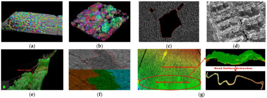
Figure 1. Demonstration of modelling for LiDAR data analysis of forest resources. (a) Individual tree segmentation, (b) tree species identification, (c) water source identification, (d) building identification, (e) powerline hazard point identification, (f) separation zone identification, (g) understory road identification.

2.2. Tri-14 CA Space Model for Crowd Evacuation Simulation

Cellular automata are dynamical systems defined on a cellular space composed of cells with discrete, finite states, evolving over discrete time dimensions according to certain local rules. They possess the capability to simulate the spatiotemporal evolution of complex systems [38]. In fact, studies on forest fire spread simulation based on cellular automata have been very common in recent years [39,40,41,42,43,44].

The traditional spatial division methods of two-dimensional cellular automata typically include three types: triangular, quadrilateral, and hexagonal meshes, usually corresponding to regular polygons, with specific arrangements depicted in Figure 2. Each has its advantages and disadvantages in terms of the number of neighbors, computer representation and display, and the simulation of isotropic phenomena, as shown in Table 1 [45]. Taking the widely adopted two-dimensional square grid as an example, the neighbor configuration of cellular automata can mainly be classified into three types: Von Neumann type, Moore type, and extended Moore type, as shown in Figure 3, where the blue grids represent the object cells and the red grids represent their corresponding neighbors. For the non-expanding CA models of regular triangular, square and hexagonal grids, the number of Von Neumann-type neighbors for the cells is 3, 4 and 6, respectively, while the Moore-type neighbor numbers are 12, 8 and 6, respectively. When using cellular automata for simulation, the Moore-type neighborhood is more commonly adopted because it has a larger number of neighbors.

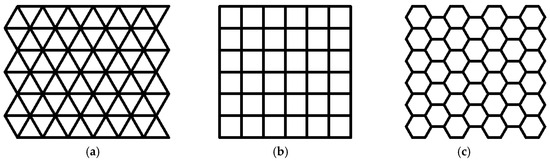
Figure 2. Traditional 2D cellular spatial meshing. (a) Equilateral triangle, (b) regular quadrangle, (c) regular hexagon.

Table 1. Advantages and disadvantages of different types of mesh in cellular automata.

Grid Type	Advantage	Disadvantages
Equilateral triangle	It has fewer neighbors and is very useful at certain times.	It is not convenient for computer expression and display.
Regular quadrangle	It is intuitive and simple, and is very suitable for computer expression and display.	It cannot simulate the isotropic phenomenon well.
Regular hexagon	It can simulate the isotropic phenomenon quite well.	It is difficult and complex in computer expression and display.

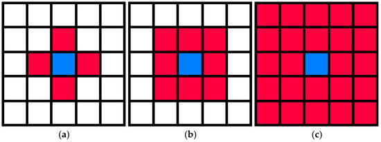
Figure 3. Common neighbor types of two-dimensional cellular automata model. (a) Von Neumann type (r = 1), (b) Moore type (r = 1), (c) Extended Moore type (r = 2).

Tri-14 is also a typical CA model used for simulating crowd evacuation [46,47]. However, its spatial division method differs from those of traditional two-dimensional cellular automata. It divides a square into several interconnected isosceles right triangles using a method reminiscent of the Chinese character “米,” resulting in four types of configurations. Figure 4 shows the spatial mesh division method and the Moore-type neighbors in the Tri-14 model, where blue and red triangular blocks represent the object cells in four different occupancy situations and their 14 neighboring cells, respectively. The most significant advantage and feature of the Tri-14 evacuation model is that it increases the evacuation directions of a single person in the barrier-free state to 14, while in the traditional square-cell automata, the value is 8 when using Moore-type neighbors. This significantly enhances the freedom of crowd evacuation and enables more accurate and realistic representation of the behavior characteristics of crowd evacuation direction selection. In addition, compared with the traditional triangular CA model using the Moore neighborhood, one advantage of the Tri-14 model lies in the fact that its neighborhood number is 14, which is greater than the 12 neighborhoods of the traditional triangular CA model. More importantly, the traditional triangular CA model is not convenient for computer expression, while the Tri-14 model can be easily expressed in a plane by using a three-dimensional array. Therefore, the spatial cellular automata grid division method for forest fire spread in this study draws on the Tri-14 model, which can greatly expand the number of possible directions for forest fire spread, making the calculation of surface fire spread more accurate and the visualization effect closer to reality.

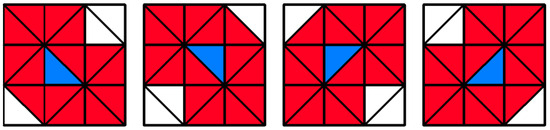
Figure 4. Neighbors of triangular mesh cellular automata in the Tri-14 model in four different positioning scenarios.

2.3. Wang Zhengfei Model of Surface Fire Spread Speed and Its Improvement

The Wang Zhengfei model selects fuel type, wind speed, and slope as the primary influencing factors to predict surface fire spread [13]. Based on extensive experimental data, this model is statistical in nature. The basic equation for surface fire spread speed in the Wang Zhengfei model is as follows:

R = R₀K_wK_s/cosα,

(1)

where R represents the estimated fire spread speed (m/min); R₀ denotes the initial spread speed (m/min); K_w is the wind speed correction factor; K_s is the fuel arrangement correction factor; cosα is the average ground slope correction factor; and α indicates the slope.

Referencing international work by Lawson, Mao Xianmin introduced the Spread Factor (SF), combined with the Canadian National Fire Prediction System experiment, the term 1/cosα in the above equation was rewritten as K_φ, named the terrain influence factor [28]. The equation is thus modified to:

R = R₀K_sK_wK_φ,

(2)

(1) Initial spread speed R₀

R₀ is data obtained from indoor combustion (or no wind) conditions, calculated as R₀ = L/t, where L is the maximum distance from the ignition point to the fire front (m), and t is the time (min). Based on collected meteorological data, forest fire data, and microclimate observation raw data, Zhang Xiaoting and Liu Peishun considered only the impact of fuel moisture, using an exponential function as the empirical regression equation type [29]. The relationship between fuel moisture m and initial spread speed R₀ is obtained through simple linear regression, improving prediction efficiency:

R₀ = 1.0372e^−0.057m,

(3)

(2) Fuel arrangement correction factor K_s

The fuel arrangement correction factor K_s represents the flammability (chemical properties) and the burning-favorable arrangement (physical properties) of the fuel, which can be assumed constant for a given time and place. The value of K_s can be determined from Table 2.

Table 2. Value of fuel arrangement correction factor K_s [36].

Fuel type	Flat Coniferous Forest	Korean Pine China Armand Pine	Deadwood Shatter	Couch Grass and Ruderal	Earth Almona Betula Japonica	Grassland
Ks	0.8	1.0	1.2	1.6	1.8	2.0

(3) Wind speed correction factor K_w

Generally, the direction of the wind aligns with the spread direction of the fire front, directly affecting the surface fire spread speed. Based on Wang Zhengfei’s experimental records on surface fire spread, an exponential function is used as the empirical regression equation type. Mao Xianmin (The role of wind and terrain on the rate of spread of surface fire) obtained an empirical formula for the relationship between wind speed and fire speed using simple linear regression:

K_w = e^0.1783v,

(4)

(4) Terrain influence factor K_φ

Slope and aspect in the terrain are also major factors influencing surface fire spread speed. Considering the combination of wind direction and terrain, Mao Xianmin and others further refined the slope influence factor K_φ, deriving equations for uphill, downhill, left-level slope, right-level slope, and wind direction, making the model more applicable to reality. This model is widely used in current surface fire spread scenarios. Subsequently, based on the studies of the aforementioned scholars, Ma Fei et al. established a mathematical model for forest fire spread based on the octree theory, and the calculated modes of terrain influence factor K_φ in the model are shown in Table 3, where φ is the angle of terrain slop [30].

Table 3. Terrain influence factor related to eight different spreading directions.

Directional Terrain Type	Terrain Influence Factor Kφ
Uphill	exp[3.533(tanφ)1.2]
Right uphill	exp{3.533[tan(φ × cos45°)]1.2}
Right-flat slope	1
Right downhill	exp{−3.533[tan(φ × cos45°)]1.2}
Downhill	exp[−3.533(tanφ)1.2]
Left downhill	exp{−3.533[tan(φ × cos(−45°))]1.2}
Left-flat slope	1
Left uphill	exp{3.533[tan(φ × cos(−45°))]1.2}

Furthermore, by simple linear regression, Zhang Xiaoting and others [29] obtained the linear regression model formula for slope and the influence factor K_φ as:

K_φ = 0.0249w + 1 = 0.0249tanφ + 1 (w ≤ 0),

(5)

K_φ = 0.6172e^0.00805w = 0.6172e^0.00805tanφ (w ≤ 0),

(6)

where w is the slope, and φ is the angle of terrain slop.

3. Basic Techniques and Models

3.1. Surface Fire Spread Speed Model

Generally, a hillside forest landscape is as depicted in the figure. “O” represents the ignition point, “U” the peak, “$\overrightarrow{OU}$, $\overrightarrow{OD}$, $\overrightarrow{OL}$, $\overrightarrow{OR}$” the directions of uphill, downhill, left-flat slope, and right-flat slope, with the wind blowing in any direction. The figure illustrates wind directions in the four quadrants. Rotate “$OU$” clockwise, when it aligns with the wind direction v, let the angle of rotation be equal to θ, as shown in Figure 5.

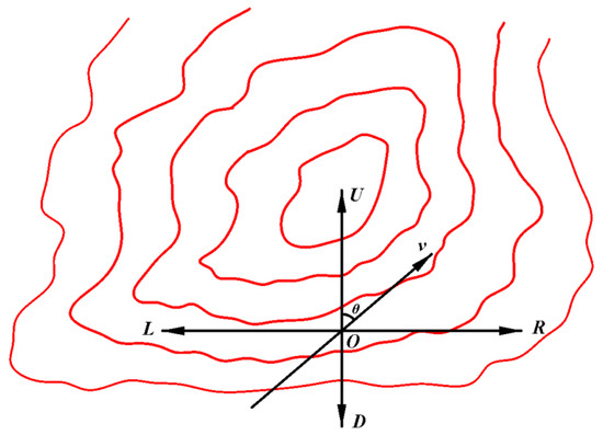
Figure 5. Wind direction and terrain schematic diagram (the red curve represents contour lines) [28].

Herein, integrating the research findings on fire spread speed mathematical models by Wang Zhengfei, Mao Xianmin, Zhang Xiaoting, Ma Fei et al., along with the Tri-14 isosceles triangle mesh division method and Moore-type neighbor model [13,28,29,30], based on the first object cell from the left in Figure 4, with specific directions for uphill, downhill, and left and right level slopes as shown in Figure 5, the following wind speed correction factors and terrain influence factors for fire spread from the object cell to its surrounding neighbors are proposed by utilize interpolation method, as shown in Table 4. The direction codes in the first column of Table 4 are consistent with the 14 red neighboring cells of the blue object cells marked in Figure 6. The Table 4 also lists the spread distances for each direction, which are the length of the line connecting the centroid of the object cell triangle and the centroid of the corresponding neighboring cell triangles (L represents the length of the two equal sides of an individual isosceles right triangle cell mesh, as indicated in Figure 6, here referred to as “mesh metric edge length”). The meanings of the parameters and variables in Table 4 and the equations are as discussed in the previous section. The basic equation for forest fire spread speed, combining wind and terrain, follows Mao Xianmin’s Formula (2). The basic equations for fire spread speed in 14 different directions under other three forms of cells and different uphill direction conditions can be similarly derived.

Table 4. Calculation parameters related to different spreading directions.

Direction Code	Directional Terrain Type	Wind Speed Correction Factor Kw	Terrain Influence Factor Kφ	Spread Distance
1	Uphill	exp(0.1783vcosθ)	exp[3.533(tanφ)1.2]	4L/3
2	Right uphill	exp[0.1783vcos(θ − 18°)]	exp{3.533[tan(φ × cos18°)]1.2}	$\sqrt{10}$L/3
3	Right uphill	exp[0.1783vcos(θ − 45°)]	exp{3.533[tan(φ × cos45°)]1.2}	$\sqrt{2}$L/3
4	Right uphill	exp[0.1783vcos(θ − 72°)]	exp{3.533[tan(φ × cos72°)]1.2}	$\sqrt{10}$L/3
5	Right-flat slope	exp[0.1783vcos(θ − 90°)]	1	4L/3
6	Right downhill	exp[0.1783vcos(θ − 117°)]	exp{−3.533[tan(φ × cos63°)]1.2}	$2\sqrt{5}$L/3
7	Right downhill	exp[0.1783vcos(θ − 135°)]	exp{−3.533[tan(φ × cos45°)]1.2}	$\sqrt{2}$L
8	Right downhill	exp[0.1783vcos(θ − 162°)]	exp{−3.533[tan(φ × cos18°)]1.2}	$\sqrt{10}$L/3
9	Downhill	exp[0.1783vcos(θ − 180°)]	exp[−3.533(tanφ)1.2]	2L/3
10	Left downhill	exp[0.1783vcos(θ − 225°)]	exp{−3.533[tan(φ × cos45°)]1.2}	$2\sqrt{2}$L/3
11	Left-flat slope	exp[0.1783vcos(θ − 270°)]	1	2L/3
12	Left uphill	exp[0.1783vcos(θ − 288°)]	exp{3.533[tan(φ × cos72°)]1.2}	$\sqrt{10}$L/3
13	Left uphill	exp[0.1783vcos(θ − 315°)]	exp{3.533[tan(φ × cos45°)]1.2}	$\sqrt{2}$L
14	Left uphill	exp[0.1783vcos(θ − 333°)]	exp{3.533[tan(φ × cos27°)]1.2}	$2\sqrt{5}$L/3

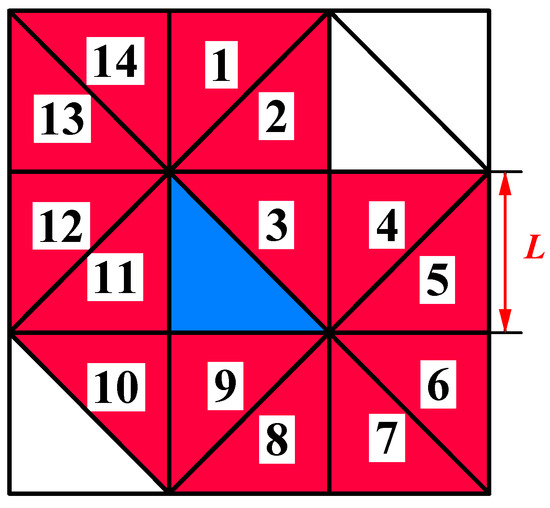
Figure 6. Annotated sequence numbers of surface fire spread direction in cellular space.

3.2. Algorithm and Function of Surface Fire Spread and Diffusion

The flowchart of surface fire spread and diffusion algorithm used in this paper is shown in Figure 7, and the interface of model software is shown in Figure 8.

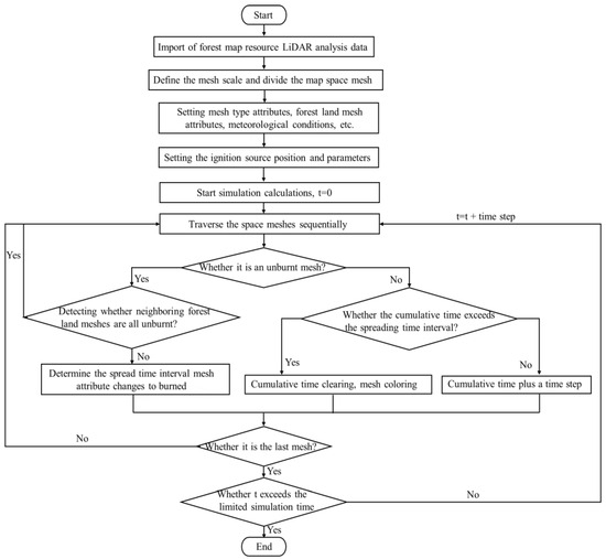
Figure 7. Flowchart of surface fire spread and diffusion algorithm.

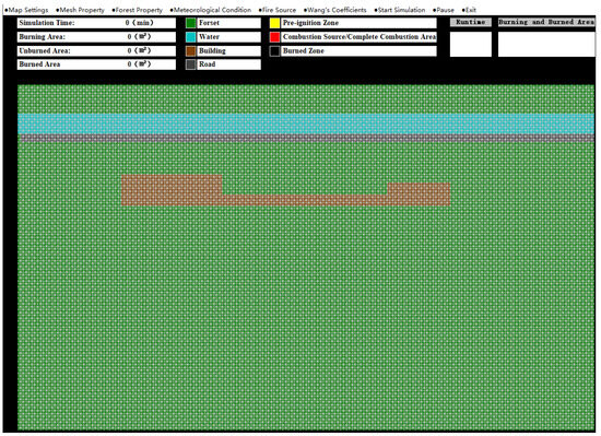
Figure 8. Model software interface.

The mountain data parameters required in the spread software model can be acquired through the map preprocessing technologies described in Section 2.1 or set and adjusted in a customized manner. The cell mesh scale can be determined comprehensively based on the map scale and simulation accuracy requirements, with a default time step of 1 min, which can be modified according to practical needs. The mesh type attributes in this software model are categorized into four types: forest land, water bodies, roads, and buildings, which are filled and displayed in green, blue, gray, and brown, respectively, on the display interface and can be set through areal or clicking methods. Forest land attribute settings mainly include stand structure, vegetation type, and plant moisture content. Meteorological condition parameters mainly encompass temperature, air humidity, wind direction, and wind speed. Ignition sources (including point and area sources) can be set according to their types. During the simulation process, the software interface can display in real time parameters such as simulation time, burned area, actively burning area, and unburned area, and it is possible to export related data after the simulation ends. The burning status of the mesh is defined as pre-burn, fully burned, and extinguished, represented by yellow, red, and black filling of the corresponding cell mesh, respectively, enabling real-time observation of images such as ignition areas, fire front, and fire line. The extinguishing time can be input based on experimental or actual measurement data. The initial spread speed can be estimated based on experimental values or using Formula (3). The terrain influence factor can be selected using the Mao Xianmin or Zhang Xiaoting model. Simulation modes include both time-limited and unlimited time modes. Additionally, it should be noted that in the algorithm model, the mesh cumulative time, calculated from different spread direction paths, needs to be determined and the shortest cumulative time among them is used as the cumulative time item in the algorithm.

4. Discussion

4.1. Basic Condition and Parameter Setting of Examples

Several demonstration examples using this model software are conducted, with the relevant key parameter configurations provided in Table 5. For these examples, the uphill direction, forest land size, mesh metric edge length, simulation time step, simulation time limit, initial spread speed, and the fuel arrangement correction factor K_s are all assigned the same values. The terrain influence factor is determined based on the Mao Xianmin calculation model, and it is calculated by converting according to the terrain slope angle specified in the corresponding examples.

Table 5. Basic condition and parameter setting of examples.

Uphill Direction	Forest Land Size	Mesh Metric Edge Length L	Simulation Time Step
East	100 hm × 100 hm	100 m	1.5 min
Simulation time limit	Initial spread speed R0	Fuel arrangement correction factor Ks	Terrain influence factor Kφ
12 h/720 min	1 m/min (Experimental value)	1.0 (Korean Pine)	Mao Xianmin calculation model
Series numbers	Wind speed v	Angle of rotation of wind direction θ	Terrain slope angle φ
1	0	0°	0°
2	2 m/s	0°	0°
3	4 m/s	0°	0°
4	0	0°	10°
5	0	0°	20°
6	2 m/s	45°	20°
7	2 m/s	90°	20°
8	2 m/s	180°	20°
9	4 m/s	0°	20°

4.2. Example Run Visual Effect Demonstration

According to the series numbers shown in Table 5, the visualization of the running effects for each example is provided in Table 6. The row corresponding to series number 0 shows the initial running state, including the location of the ignition point and relevant descriptions.

Table 6. Example run visual effect demonstration.

Series Numbers	Data and Images
0		t = 0 Uniform initial fire source overfire area S = 4 hm2 The intersection of the blue lines indicates the centre of the ignition point. The red colour indicates the combustion source or complete combustion area. The yellow colour indicates the pre-ignition zone, which can be interpreted as the line of fire.
1
	t = 120 min, overfire area S = 12 hm2	t = 240 min, overfire area S = 28 hm2	t = 360 min, overfire area S = 60 hm2
	t = 480 min, overfire area S = 100 hm2	t = 600 min, overfire area S = 156 hm2	t = 720 min, overfire area S = 228 hm2
2
	t = 120 min, overfire area S = 15 hm2	t = 240 min, overfire area S = 38 hm2	t = 360 min, overfire area S = 78 hm2
	t = 480 min, overfire area S = 132 hm2	t = 600 min, overfire area S = 203 hm2	t = 720 min, overfire area S = 288 hm2
3
	t = 120 min, overfire area S = 14 hm2	t = 240 min, overfire area S = 49 hm2	t = 360 min, overfire area S = 106 hm2
	t = 480 min, overfire area S = 186 hm2	t = 600 min, overfire area S = 289 hm2	t = 720 min, overfire area S = 419 hm2
4
	t = 120 min, overfire area S = 14 hm2	t = 240 min, overfire area S = 43 hm2	t = 360 min, overfire area S = 80 hm2
	t = 480 min, overfire area S = 143 hm2	t = 600 min, overfire area S = 226 hm2	t = 720 min, overfire area S = 324 hm2
5
	t = 120 min, overfire area S = 23 hm2	t = 240 min, overfire area S = 77 hm2	t = 360 min, overfire area S = 160 hm2
	t = 480 min, overfire area S = 279 hm2	t = 600 min, overfire area S = 433 hm2	t = 720 min, overfire area S = 602 hm2
6
	t = 120 min, overfire area S = 33 hm2	t = 240 min, overfire area S = 114 hm2	t = 360 min, overfire area S = 230.5 hm2
	t = 480 min, overfire area S = 415 hm2	t = 600 min, overfire area S = 644 hm2	t = 720 min, overfire area S = 894.5 hm2
7
	t = 120 min, overfire area S = 22.5 hm2	t = 240 min, overfire area S = 79.5 hm2	t = 360 min, overfire area S = 174.5 hm2
	t = 480 min, overfire area S = 306.5 hm2	t = 600 min, overfire area S = 459 hm2	t = 720 min, overfire area S = 661 hm2
8
	t = 120 min, overfire area S = 14 hm2	t = 240 min, overfire area S = 47 hm2	t = 360 min, overfire area S = 95 hm2
	t = 480 min, overfire area S = 161 hm2	t = 600 min, overfire area S = 246 hm2	t = 720 min, overfire area S = 344 hm2
9
	t = 120 min, overfire area S = 53 hm2	t = 240 min, overfire area S = 200 hm2	t = 360 min, overfire area S = 428 hm2
	t = 480 min, overfire area S = 743 hm2	t = 600 min, overfire area S = 1131 hm2	t = 720 min, overfire area S = 1638 hm2

4.3. Model Error Analysis

To investigate the error of this model, the initial parameters for series number 1 in Table 5 were used to run the model for 960 min. The results obtained from this model, the Von Neumann and Moore type cellular automata models, and the continuous model theoretical values for the overfire area (results are rounded to one decimal place) were compared. It should be noted that in this example, the continuous model refers to an expansion model where the overfire area is formed by taking the fire source point as the center and with the defined spread speed and simulation time as the radius for the spread. The runtime was set to 960 min, and the related results are presented in Table 7 and Figure 9.

Table 7. Model error analysis.

Time (min)	Overfire Area in Continuous Model (hm2)	Overfire Area in Tri-14 Model	Absolute Value of Relative Error	Overfire Area in Von Neumann Model	Absolute Value of Relative Error	Overfire Area in Moore Model	Absolute Value of Relative Error
0	4.0	4	—	4	—	4	—
120	17.0	12	29.54%	12	29.54%	12	29.54%
240	39.1	28	28.41%	24	38.64%	24	38.64%
360	70.2	60	14.58%	40	43.05%	52	25.97%
480	110.4	100	9.43%	60	45.66%	80	27.55%
600	159.6	156	2.28%	112	29.84%	132	17.31%
720	217.9	228	4.63%	144	33.92%	176	19.23%
840	285.2	288	0.97%	180	36.89%	232	18.66%
960	361.6	380	5.09%	220	39.16%	300	17.03%

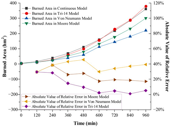
Figure 9. Comparison chart of changes in overfire area and related errors of different models.

From the data in Table 5 and Figure 8, and its variation over time, it can be observed that under the condition that the ignition states are identical and the wind speed and terrain slope angle are 0, compared with the calculated values of over fire area in the continuous surface fire spread theoretical model, the model proposed in this paper, which is based on the Tri-14 cellular automata spatial mesh division method, demonstrates the best consistency between the time-varying curve of the burned area and the theoretical calculation curve over time, followed by the Moore type model, with the Von Neumann type model showing the least consistency.

Looking from the perspective of the absolute value of the relative error, in the early stages of the run time, the related errors of all three CA models are at a higher level. As the run time progresses, the relative error values decrease, eventually fluctuating within a very small range or slightly decreasing or increasing around a certain level. This can be interpreted as a “relative error stable segment,” which, in this case, can be considered to occur after 600 s. Within this “relative error stable segment,” the smallest relative error value belongs to the model proposed in this paper, with the absolute value of relative error fluctuating around 3%. The Moore type CA model has the next smallest relative error, while the Von Neumann type model has the largest average relative error, exceeding 30% and showing a gradual slight increase over time. Therefore, from the perspectives of the time-varying curve of the burned area and relative error, the model constructed in this paper demonstrates significantly higher calculation accuracy than the traditional Moore and Von Neumann type surface fire spread models. Moreover, as the limited simulation duration increases, the accuracy of this model becomes more pronounced.

5. Conclusions

(1) This study applies the Tri-14 crowd evacuation model’s cellular automata triangle mesh division method and its neighbor arrangement to the surface fire spread cellular automata model, expanding the traditional surface fire spread CA model’s directions from 4 or 8 to 14. This enhancement improves the visualization of the surface fire spread process.

(2) Based on Wang Zhengfei’s and related improved mathematical statistical speed models for surface fire spread, this research constructs wind speed correction factors and terrain influence factors suitable for 14 directions under different occupancy configurations, combined with a spatial model.

(3) On the foundation of the spatial and statistical speed models, this study has developed a visual simulation software through computer programming. It can utilize relevant forest resources map preprocessing technologies for acquiring and embedding mountain-related parameters. The software features good dynamic display, low dependency on parameters, and high computational efficiency.

(4) The output results from related fundamental examples indicate that the model constructed in this research significantly surpasses traditional CA surface fire spread models in calculation accuracy. Moreover, as the limited simulation duration increases, its precision becomes even more pronounced.

(5) In addition, in order that the model and methodology presented in this paper can be transferred into practice, a lot of work is needed in future research including the collection and processing of forest map resource data, as well as the correction of relevant parameters through comparative analysis with actual fire cases and existing software.

References

- Global Forest Resources Assessment 2020. Available online: https://www.fao.org/forest-resources-assessment/past-assessments/fra-2020 (accessed on 20 March 2023).
- Tencent. Available online: https://new.qq.com/rain/a/20230321A05K5A00 (accessed on 21 March 2023).
- Yan, Z.C. Forest and Grass Fire Detection Based on UAV Vision. Ph.D. Thesis, Northeast Forestry University, Harbin, China, 2023. [Google Scholar] [CrossRef]
- Long, T.T.; Yin, J.Y.; Ou, Z.R.; Yang, Q.; Li, Y.; Wang, Q.H. Comprehensive Assessment and Spatial Pattern Study on Forest Fire Risk in Yunnan Province. China Saf. Sci. J. 2021, 31, 167–173. [Google Scholar] [CrossRef]
- Ghali, R.; Akhloufi, M.A.; Jmal, M.; Mseddi, W.S.; Attia, R. Forest Fires Segmentation using Deep Convolutional Neural Networks. In Proceedings of the 2021 IEEE International Conference on Systems, Man, and Cybernetics (SMC), Melbourne, Australia, 17–20 October 2021; pp. 2109–2114. [Google Scholar] [CrossRef]
- Popular Science—A Forest Fire Prevention Guide. Available online: https://www.thepaper.cn/newsDetail_forward_22310147 (accessed on 2 August 2025).
- China’s Forest Fires: A Decade of Progress in Prevention and Control. Available online: https://www.thepaper.cn/newsDetail_forward_13665038 (accessed on 21 July 2021).
- Wang, Y.H.; Yang, X.D.; Ren, L.W.; Yuan, X.Y.; Liang, L.; Zhao, L.Q. Research progress of wildfire spread model and its applicability. Sci. Technol. Rev. 2023, 41, 49–57. [Google Scholar] [CrossRef]
- Sun, J.; Qi, W.; Huang, Y.; Xu, C.; Yang, W. Facing the Wildfire Spread Risk Challenge: Where Are We Now and Where Are We Going? Fire 2023, 6, 228. [Google Scholar] [CrossRef]
- Burgan, R.E. BEHAVE: Fire Behavior Prediction and Fuel Modeling System, Fuel Subsystem; U.S. Department of Agriculture, Forest Service, Intermountain Forest and Range Experiment Station: Ogden, UT, USA, 1984; Part 1. [Google Scholar]
- Linn, R.R. A Transport Model for Prediction of Wildfire Behaviour. Ph.D. Thesis, New Mexico State University, Las Cruces, NM, USA, 2018. [Google Scholar]
- Mell, W.; Jenkins, M.A.; Gould, J.; Cheney, P. A physics-based approach to modelling grassland fires. Int. J. Wildland Fire 2007, 16, 1–22. [Google Scholar] [CrossRef]
- Wang, Z.F. The measurement method of the wildfire initial spread rate. Mt. Res. 1983, 2, 42–51. [Google Scholar] [CrossRef]
- Clark, T.L.; Jenkins, M.A.; Coen, J.; Latham, D. A coupled atmosphere-fire model: Convective feedback on fire-line dynamics. J. Appl. Meteorol. Climatol. 1996, 35, 875–901. [Google Scholar] [CrossRef]
- Clark, T.L.; Coen, J.; Latham, D. Description of a coupled atmosphere-fire model. Int. J. Wildland Fire 2004, 13, 49–64. [Google Scholar] [CrossRef]
- Mesoscale and Microscale Meteorology Laboratory of NCAR. Weather Research & Forecasting Model (WRF). Available online: https://www.mmm.ucar.edu/wrf-model-general (accessed on 10 August 2024).
- Hu, X.; Sun, Y.; Ntaimo, L. DEVS-FIRE: Design and Application of Formal Discrete Event Wildfire Spread and Suppression Models. Simulation 2012, 88, 259–279. [Google Scholar] [CrossRef]
- Ntaimo, L.; Zeigler, B.P.; Vasconcelos, M.J.; Khargharia, B. Forest Fire Spread and Suppression in DEVS. Simulation 2004, 80, 479–500. [Google Scholar] [CrossRef]
- Filippi, J.B.; Mallet, V.; Nader, B. Evaluation of Forest Fire Models on a Large Observation Database. Nat. Hazards Earth Syst. Sci. 2014, 14, 3077–3091. [Google Scholar] [CrossRef]
- Lafore, J.P.; Stein, J.; Asencio, N.; Bougeault, P.; Ducrocq, V.; Duron, J.; Fischer, C.; Héreil, P.; Mascart, P.; Masson, V.; et al. The Meso-NH Atmospheric Simulation System. Part I: Adiabatic Formulation and Control Simulations. In Annales Geophysicae; Springer: Göttingen, Germany, 1998; Volume 16, pp. 90–109. [Google Scholar] [CrossRef]
- Pastor, E.; Zarate, L.; Planas, E.; Arnaldos, J. Mathematical models and calculation systems for the study of wildland fire behaviour. Prog. Energy Combust. Sci. 2003, 29, 139–153. [Google Scholar] [CrossRef]
- Or, D.; Furtak-Cole, E.; Berli, M.; Shillito, R.; Ebrahimian, H.; Vahdat-Aboueshagh, H.; McKenna, S.A. Review of wildfire modeling considering effects on land surfaces. Earth-Sci. Rev. 2023, 245, 104569. [Google Scholar] [CrossRef]
- Bakhshaii, A.; Johnson, E.A. A review of a new generation of wildfire–atmosphere modeling. Can. J. For. Res. 2019, 49, 565–574. [Google Scholar] [CrossRef]
- Fons, W.L. Analysis of fire spread in light forest fuels. J. Agric. Res. 1946, 72, 93–121. [Google Scholar]
- Albini, F.A. Wildland fire spread by radiation: A model including fuel cooling by natural convection. Combust. Sci. Technol. 1986, 45, 101–113. [Google Scholar] [CrossRef]
- De Mestre, N.J.; Catchpole, E.A.; Anderson, D.H.; Rothermel, R.C. Uniform propagation of a planar fire front without wind. Combust. Sci. Technol. 1989, 65, 231–244. [Google Scholar] [CrossRef]
- McArthur, A.G. Weather and Grassland Fire Behavior; Forestry and Timber Bureau, Department of National Development, Commonwealth of Australia: Canberra, Australia, 1966. [Google Scholar]
- Mao, X.M. The influence of wind and relief on the speed of the forest fire spreading. Q. J. Appl. Meteorol. 1993, 4, 100–104. [Google Scholar]
- Zhang, X.T.; Liu, P.S.; Wang, X.F. Research on Improvement of Wang Zhengfei’s Forest Fire Spread Model. Shandong For. Sci. Technol. 2020, 50, 1–6+40. [Google Scholar]
- Ma, T.; Zheng, J.; Wang, Z.C. Informatization Research on Forest Fire Spread Model of Forest Sub-compartment. For. Inventory Plan. 2013, 38, 55–59+64. [Google Scholar] [CrossRef]
- Rothermel, R.C. A Mathematical Model for Predicting Fire Spread in Wildland Fuels; Research Paper INT-115; Intermountain Forest & Range Experiment Station, Forest Service, US Department of Agriculture: Washington, DC, USA, 1972; Volume 40, p. 1972. [Google Scholar]
- Ascoli, D.; Vacchiano, G.; Motta, R.; Bovio, G. Building Rothermel fire behaviour fuel models by genetic algorithm optimisation. Int. J. Wildland Fire 2015, 24, 317–328. [Google Scholar] [CrossRef]
- Finney, M.A. FARSITE: Fire Area Simulator-Model Development and Evaluation; U.S. Department of Agriculture, Forest Service, Rocky Mountain Research Station: Fort Collins, CO, USA, 1998. [Google Scholar]
- Ramirez, J.; Monedero, S.; Buckley, D. New approaches in fire simulations analysis with Wildfire Analyst. In Proceedings of the the 5th International Wildland Fire Conference, Sun City, South Africa, 9–13 May 2011. [Google Scholar]
- Monedero, S.; Ramirez, J.; Cardil, A. Predicting fire spread and behaviour on the fireline. Wildfire analyst pocket: A mobile app for wildland fire prediction. Ecol. Model. 2019, 392, 103–107. [Google Scholar] [CrossRef]
- Tian, Y.P.; Jin, C.Y.; Wang, B.; Li, M.Z. Forest Fire Spread Prediction Based on Improved Wang Zhengfei Model Combined with Cellular Automata. J. Cent. South Univ. For. Technol. 2024, 44, 14–25. [Google Scholar]
- Zhu, L. Comparison of Forest Fire Simulation Based on Wang Zhengfei’s Model and Rothermel Model. Agric. Sci. Technol. Inf. 2019, 3, 85–88. [Google Scholar] [CrossRef]
- Burks, A.W. Von Neumann’s Self-Reproducing Automata; University of Illinois Press: Urbana, IL, USA, 1970; pp. 3–64. [Google Scholar]
- Mastorakos, E.; Gkantonas, S.; Efstathiou, G.; Giusti, A. A hybrid stochastic Lagrangian-cellular automata framework for modelling fire propagation in inhomogeneous terrains. Proc. Combust. Inst. 2023, 39, 3853–3862. [Google Scholar] [CrossRef]
- Byari, M.; Bernoussi, A.; Jellouli, O.; Ouardouz, M.; Amharref, M. Multi-scale 3D cellular automata modeling: Application to wildland fire spread. Chaos Solitons Fractals 2022, 164, 112653. [Google Scholar] [CrossRef]
- Gharakhanlou, N.M.; Hooshangi, N. Dynamic simulation of fire propagation in forests and rangelands using a GIS-based cellular automata model. Int. J. Wildland Fire 2021, 30, 652–663. [Google Scholar] [CrossRef]
- Trucchia, A.; D’Andrea, M.; Baghino, F.; Fiorucci, P.; Ferraris, L.; Negro, D.; Gollini, A.; Severino, M. PROPAGATOR: An Operational Cellular-Automata Based Wildfire Simulator. Fire 2020, 3, 26. [Google Scholar] [CrossRef]
- Zhang, S.Y.; Liu, J.Q.; Gao, H.W.; Chen, X.D.; Li, X.D.; Hua, J. Study on Forest Fire spread Model of Multi-dimensional Cellular Automata based on Rothermel Speed Formula. Cerne 2021, 27, e-102932. [Google Scholar] [CrossRef]
- Meng, Q.K.; Huai, Y.J.; You, J.W.; Nie, X.Y. Visualization of 3D forest fire spread based on the coupling of multiple weather factors. Comput. Graph. UK 2023, 110, 58–68. [Google Scholar] [CrossRef]
- Lu, L.G. A Research on the Influence Mechanism of Narrow and Long Panel-like Obstacles on Pedestrian Evacuation Characteristics Under Different Initial Crowd Density Conditions. Ph.D. Thesis, China University of Mining and Technology, Xuzhou, China, 2024. [Google Scholar]
- Ji, J.W.; Lu, L.G.; Jin, Z.H.; Wei, S.P.; Ni, L. A cellular automata model for high-density crowd evacuation using triangle grids. Phys. A Stat. Mech. Its Appl. 2018, 509, 1034–1045. [Google Scholar] [CrossRef]
- Lu, L.G.; Ji, J.; Zhai, C.; Wang, S.C.; Zhang, Z.; Yang, T.T. Research on the Influence of Narrow and Long Obstacles with Regular Configuration on Crowd Evacuation Efficiency Based on Tri-14 Model with an Example of Supermarket. Fire 2022, 5, 164. [Google Scholar] [CrossRef]
Disclaimer/Publisher’s Note: The statements, opinions and data contained in all publications are solely those of the individual author(s) and contributor(s) and not of MDPI and/or the editor(s). MDPI and/or the editor(s) disclaim responsibility for any injury to people or property resulting from any ideas, methods, instructions or products referred to in the content. |
© 2025 by the authors. Licensee MDPI, Basel, Switzerland. This article is an open access article distributed under the terms and conditions of the Creative Commons Attribution (CC BY) license (https://creativecommons.org/licenses/by/4.0/).