Article

Evaluation of Topographic Effect Parameterizations in Weather Research and Forecasting Model over Complex Mountainous Terrain in Wildfire-Prone Regions

1
Department of Earth, Environmental & Space Sciences, Chungnam National University, Daejeon 34134, Republic of Korea
2
Institute for Earth, Computing, Human and Observing, Chapman University, Orange, CA 92866, USA
3
New and Renewable Energy Resource Map Laboratory, Korea Institute of Energy Research, Daejeon 34129, Republic of Korea
4
Ecosystem-Atmosphere Process Lab, Department of Atmospheric Sciences, Yonsei University, Seoul 03722, Republic of Korea
5
Max Planck Institute for Meteorology, 20146 Hamburg, Germany
6
Landslide Division, National Institute of Forest Science, Seoul 02455, Republic of Korea
*
Authors to whom correspondence should be addressed.
Fire 2025, 8(5), 196; https://doi.org/10.3390/fire8050196
Submission received: 20 March 2025 / Revised: 29 April 2025 / Accepted: 9 May 2025 / Published: 14 May 2025
(This article belongs to the Special Issue Dynamics of Wind-Fire Interaction: Fundamentals and Applications)

Abstract

:
Recent trends of intense forest fires in the Korean Peninsula have increased concerns about more extreme burning in the future under a warming climate. Accurate and reliable fire weather information has become more critical to reduce the risk of forest-related disasters over complex terrain. In this study, two parameterizations reflecting complex topographic effects were implemented in the Weather Research and Forecasting (WRF) model. The model performance was evaluated over the mountainous region in Gangwon-do, South Korea’s most significant forest area. The simulation results of the wildfire case in 2019 show that subgrid-scale orographic parameterization considerably improves model performance regarding wind speed, with a lower root mean square error (RMSE) and bias by 53% and 57%, respectively. Another parameterization, reflecting slope and shading, effectively reflected sunrise and sunset effects. The second parametrization produced little effect on the daily averages of meteorological elements. However, thermodynamic components such as temperature and heat flux show more realistic values during sunset or sunrise when the solar altitude angle is low. The results imply that applying topographic parameterizations is required in numerical simulations, especially for hazardous weather conditions over complex terrain in mountainous regions.

1. Introduction

South Korea has the fourth largest forest area ratio in the world, at 62.7%. Gangwon-do includes 21.6% of the total forest area, 6,298,134 ha, accounting for 81.2% of the total provincial area [1]. Gangwon-do, which is the largest forest in South Korea, is divided into the Yeongdong and Yeongseo regions based on the Taebaek Mountains, and these two regions have distinct climates. Due to its location on the leeward side of the Taebaek Mountains, the Yeongdong region frequently has strong and dry downslope winds in spring and autumn [2]. In spring, continental westerly winds bring dry conditions to the mountainous region in Korea. Due to the Korean Peninsula’s geographic location, high pressure to the south and low pressure in the north combine with the regional effect of the Taebaek Mountains, producing a Foehn effect that generates strong, dry winds. This wind generates conditions conducive to wildfires, and when they do occur, they spread rapidly and inflict major damage [3]. Meteorological phenomena in forested areas are regional and irregular, with more complex topography than on flat ground [4,5]. Furthermore, because the spatial density of surface weather stations is low in comparison to that of flatlands, such as a city with a large population [6], determining the exact spatial distribution of meteorological elements is challenging [7,8,9].
According to the Intergovernmental Panel on Climate Change (IPCC), global temperatures and sea levels are rising, and permafrost and glaciers are receding. In addition, the temperature increase rate is accelerating [10,11,12]. The effects of climate change caused by global warming are causing abnormal climates and weather conditions to occur more frequently around the world, and the damage caused by weather disasters is increasing. Extreme weather events such as heat waves, typhoons, and heavy rainfall will occur more often, increasing the likelihood of forest disasters such as wildfires and landslides. Piñol et al. [13] predicted that global warming will increase the frequency and intensity of wildfires. Weather conditions are closely related to the likelihood of wildfires [14,15]. Heatwaves and long-term droughts are particularly strong contributors to increased wildfire risk [16,17]. For example, in 2010, a heatwave in Central Russia caused wildfires near Moscow to burn more than 810,000 ha, and in 2019, wildfires in northern Siberia burned more than 3 million ha. Similarly, in Australia, wildfires that started in September 2019 due to prolonged drought continued for about 6 months, burning 19 million ha by February 2020. California, USA, is another region highly susceptible to wildfires due to its geographic characteristics, including warm and dry autumn air, delayed precipitation, and strong winds [18,19,20]. In California, approximately 400,000 ha were burned in 2017, approximately 800,000 ha in 2018, approximately 100,000 ha in 2019, and approximately 1.76 million ha in 2020.
In addition to climate and weather factors, topography is another critical element regulating wildfire dynamics. Topographic influences are particularly pronounced in complex terrains, where they significantly affect fire behavior [21]. Even under warming climate conditions and increasing fuel aridity, topography remains a major factor influencing the occurrence of large, severe wildfires [22,23]. This highlights the importance of extreme wind events, which are a major driver of large wildfires, and their role in altering near-surface wind patterns over complex terrain. Without accurate wind simulations, it becomes difficult to reliably estimate wildfire behavior, especially in regions with rugged topography.
Every year, many forest disasters occur in South Korea. According to data from the National Institute of Forest Science (NIFS), 4737 wildfires occurred from 2011 to 2020, and 11,195 ha of forest were burned. Of these, 2853 wildfires occurred from 2016 to 2020, with a burned area of 8927 ha. In the last 10 years, the latter part of the decade saw 60.2% of wildfires and 79.7% of burned forest areas. Notably, a total of 3254 ha were burned in 2019, of which 2832 ha were burned by large wildfires that lasted for two days beginning on April 4 in Gangwon-do. In 2021, a total of 327 wildfires occurred, burning 747 ha of forest. Furthermore, landslide damage of more than 50 ha has occurred every year since 2010, except in 2015. Landslide damage occurred across 814 ha in 2011 and 1343 ha in 2020. The main causes of forest fires are human activities, such as the burning of agricultural byproducts and waste, and carelessness by mountaineers. These activities can lead to large-scale forest fires, especially when combined with the weather and topographical conditions described above. As a result of this limitation in understanding the spatial distribution of meteorological factors, the implementation of a numerical weather prediction (NWP) model in forest areas is necessary to prevent forest disasters. Furthermore, the performance of the NWP model is becoming increasingly crucial in preparing for increasing forest disasters. However, due to the effect of complex terrain, it is difficult to predict meteorological factors in forest areas.
To address this issue, several studies on the parameterization of the effect of topography in the WRF model have been conducted [24,25,26,27,28,29]. The WRF model revealed a surface wind speed bias over flat regions and slopes [30,31,32,33,34]. Seo et al. [32] demonstrated that when simulating surface winds over Gangwon-do in Korea using the WRF model, the model tended to underestimate observed wind speeds under weak wind conditions and overestimate them under strong wind conditions. Similarly, Tsai et al. [33] conducted sensitivity tests of surface wind speed using three different PBL parameterizations in the WRF model and found that all schemes exhibited a positive bias.
Mass and Ovens [34] and Jiménez and Dudhia [26] developed a subgrid-scale topographic parameterization that corrected the wind speed bias induced by differently expressing the real terrain heights in the model. These studies introduced a sink term for surface drag into the momentum equation. Lee et al. [27] used the WRF model to apply the parameterization proposed by Jiménez and Dudhia [26] in studies of South Korea using a maximum horizontal resolution of 3 km; they demonstrated that improving surface wind expression also improves precipitation simulation performance in forest areas. Lim et al. [29] compared wind simulation performance over the midwestern region of South Korea using two parameterizations. As a result, both parameterizations improved the 10 m wind speed simulation performance, with the parameterization of Jimenez and Dudhia [26] outperforming the others. However, these studies focused on the summer and fall seasons, which are not active wildfire periods in Korea [27,29]. Additionally, the target regions in those studies were either the entire Korean Peninsula using coarse resolution or high-resolution domains applied to flat terrain. As such, they do not adequately capture the effects of parameterizations over complex terrain during the active fire season.
Furthermore, this study was conducted to examine the variations in solar radiation over slopes and valleys based on the solar zenith angle and the influence of topographic shadows in complex terrains [35,36,37]. Colette et al. [38] included changes in surface solar radiation based on the topographic shadow and solar zenith angle in the advanced regional prediction system (ARPS) model. Slope and shading parameterizations were also included in the fifth-generation Pennsylvania State University National Center for Atmospheric Research Mesoscale Model (MM5) and the WRF model. Arthur et al. [28] generated a more accurate simulation of the surface heat flux by applying these parameterizations to WRF-IBM.
Although numerous studies on the effects of complex topography have been conducted and numerical model parameterizations incorporating topographic effects have been developed, few studies have applied these parameterizations to South Korea. This study represents the very first attempt to apply both novel shading and slope parameterizations to mountainous regions in Korea during the fire season. In this study, the performance of the WRF model was evaluated by applying parameterizations reflecting topographic effects in Gangwon-do, South Korea’s largest forest area, to prepare for increasing forest disasters by improving the accuracy of numerical simulations over complex mountain terrain. In this study, the WRF model was selected since it is one of the most widely used numerical weather prediction models, serving both research and operational needs. Supported by a global user community, the WRF model continues to advance atmospheric science through innovations in model physics, computing technologies, and a wide range of applications.
The subgrid-scale topographic parameterization and the slope and shading parameterization were employed in this study. We conducted numerical experiments for one month (April 2019), investigated the differences caused by the parameterizations, and compared the simulation results with surface weather station observations. These procedures are described in detail in the Materials and Methods Section (Section 2). The Results Section (Section 3) presents the characteristics and performance of each parameterization, while the Concluding Remarks and Discussion Section (Section 4) offers a scientific review of the findings, discusses the study’s limitations, and outlines directions for future research.

2. Materials and Methods

2.1. Parameterizations for Terrain Effect

Jiménez and Dudhia [26] developed a subgrid-scale topographic parameterization that corrects the surface wind speed by reducing the positive bias over flatlands and slopes and the negative bias over mountain tops and hills using high-quality wind observations from the Comunidad Foral de Navarra, a complex terrain region in northeastern Iberia. The diverse distribution of observation stations across valleys, plains, and mountains made this region an ideal setting for the development and validation of the scheme. When the topography is discretized in the numerical simulation process, the topography of the model is expressed more smoothly and is different from reality. To include the effect of real terrain, they introduced a sink term, c t , determined by two indices (a non-dimensional Laplacian operator and a standard deviation of the terrain) in the momentum conservation equation:
2 h i , j = 0.25 ( h i + 1 , j + h i , j + 1 + h i 1 , j + h i , j 1 4 h i , j )
u t = c t u * 2 z u V
c t = 1 l n σ s s o α l n σ s s o + 1 α 2 h + 30 10 0 i f 2 h > 20   a n d   σ s s o < e i f 2 h > 10   a n d   σ s s o > e i f 10 > 2 h > 20   a n d   σ s s o > e i f 20 > 2 h > 30 i f 30 > 2 h
In Equation (1), h denotes the terrain elevation of the non-dimensional Laplacian operator. Compared with the surrounding grid, when 2 h i , j is positive, it indicates the presence of a valley that is lower than the surrounding grid, and if it is negative, it indicates the presence of a hill or mountain that is higher than the surrounding grid. The closer it is to 0, the more similar the grid elevation is to the surrounding grid. In Equation (2), u denotes the zonal wind component of the first model layer, V denotes the wind speed of the first model layer, u * denotes the friction speed, and z denotes the thickness of the first model layer. The added term c t is expressed as a function of the Laplacian operator 2 h and the standard deviation of the terrain σ s s o , as in Equation (3), where α is 2 h + 20 / 10 and e is the base of the natural logarithm. According to the above equations, c t reduces the wind speed in flat lands and increases it in mountains and hills.
The parameterization accounts for the effects of unresolved terrain by applying a correction for topography, which modulates the surface drag in the momentum conservation equation (e.g., Equation (2)). The additional drag component is determined by the c t factor (e.g., Equation (3)), which physically represents the modifications that orography imposes on the friction velocity compared to calculations that assume homogeneous terrain. A c t value equal to 1 indicates the use of the default WRF model configuration.
In the WRF model, the downward solar radiation fluxes (denoted by S W 0 ) of the direct and diffuse components of the grid points were assumed to be incident on a flat topography and were calculated for each horizontal grid. Applying slope and shading parameterizations following the method of [39,40], S W 0 was modified based on slope and shadow caused by the surrounding terrain:
S W a d j = D + ( 1 D ) c o s ( Z a d j ) c o s ( Z 0 ) S W 0
where S W a d j is the solar radiation corrected by the terrain effect, Z a d j represents the solar zenith angle with respect to the normal vector of the terrain, Z 0 denotes the solar zenith angle assuming flat terrain, and D is the diffuse ratio of S W 0 . When slope parameterization is applied, solar radiation is corrected based on the solar zenith angle in the grid, and solar radiation increases with increasing perpendicularity to the sun (the direction the ground faces the sun). If the line between the sun and grid points intersects with other terrains within the set shadow length when shading parameterization is applied, the shadow mask is set to 1, and c o s ( Z a d j ) becomes 0; thus, only diffusion is taken into account.

2.2. Model Description and Experimental Design

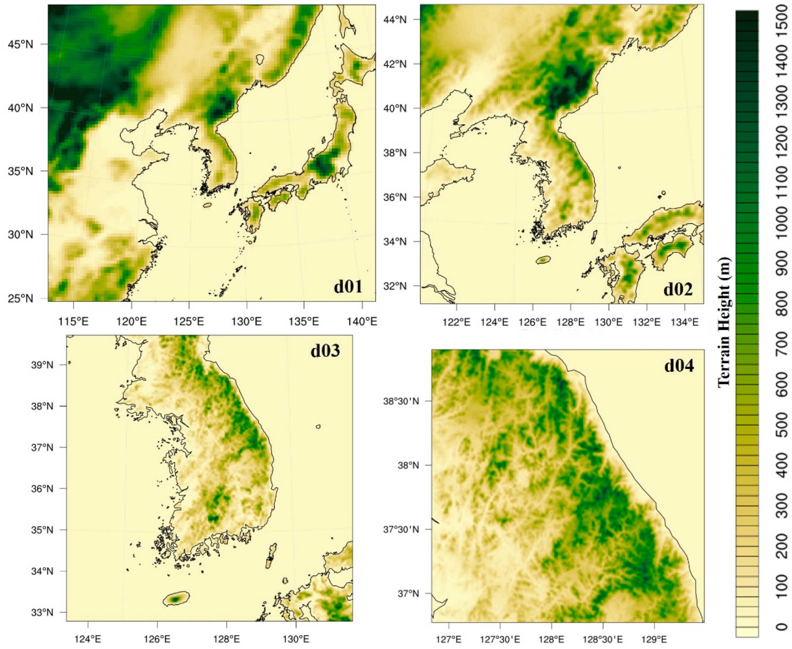
The WRF model version 3.7.1 was used to evaluate the subgrid-scale topographic parameterization and slope and shading parameterizations. The period from 31 March to 1 May 2019 was simulated, and all simulations lasted two days, including spin-up time. The initial and boundary datasets were derived from GDAS FNL with a horizontal resolution of 1° × 1° from the National Centers for Environmental Prediction/National Centers for Atmospheric Research (NCEP/NCAR) and were used at 6 h intervals. There are four domains that are one-way nested. The horizontal resolutions for domains 1 (d01), 2 (d02), 3 (d03), and 4 (d04) were 27 km, 9 km, 3 km, and 1 km, respectively. Figure 1 depicts the domain configurations, and Figure 2 shows the topographical elevation of each domain in the model.
The configuration of the WRF model is listed in Table 1. The physical parameterization employed the WRF Single-Moment 6-class microphysics scheme [41], the rapid radiative transfer model for general circulation models (RRTMG) scheme [42] for shortwave and longwave radiation, the Yonsei university (YSU) scheme [43] for planetary boundary layers, the MM5 Monin–Obukhov [44] for surface layers, and the unified Noah land surface model [45] for the land surface model. The Kain–Fritsch scheme [46] was used for cumulus parameterization and was applied only to d01 and d02 with a horizontal grid resolution of 5 km or more. Table 2 shows the results of three numerical experiments: the control run without topographic effect parameterization (CTL), the experiment with subgrid-scale topographic parameterization (TOP), and the experiment with parameterization reflecting the slope and shading effect (SSE).

2.3. Observation Data and Analysis Method

Only the results for 24 h from daily 48 h forecasts beginning at 0000 UTC were used in the numerical simulation analysis. A 15 h simulation was used for the spin-up. The analysis period was 30 days in 2019, beginning at 1500 UTC on 31 March, and ending at 1400 UTC on 30 April (1 April, 0000 LST, to 30 April, 2300 LST, 2019). To examine the parameterization reflecting the topographic effect, the horizontal distribution of simulated 2 m temperature (°C), 2 m relative humidity (%), and 10 m wind speed (m s−1), vertical distribution of simulated atmospheric temperature (°C), water vapor mixing ratio (g kg−1), and wind speed (m s−1) in each experiment were compared with the CTL experiment before comparing the results with observations (OBS). The latitude of the vertical cross-section is 37.5° N, and its longitude is 126.9–129.4° E, which encompasses Seoul, Gyeonggi-do (Hanam, Yangpyeong), Gangwon-do (Hwangseong, Pyeongchang, Gangneung), and the East Sea. Additionally, to verify the effect of the solar zenith angle on the SSE, the horizontal distribution of 2 m temperature and the vertical distribution of atmospheric temperature according to time were compared with those of the CTL experiment. Only the simulation results for d04 were analyzed.
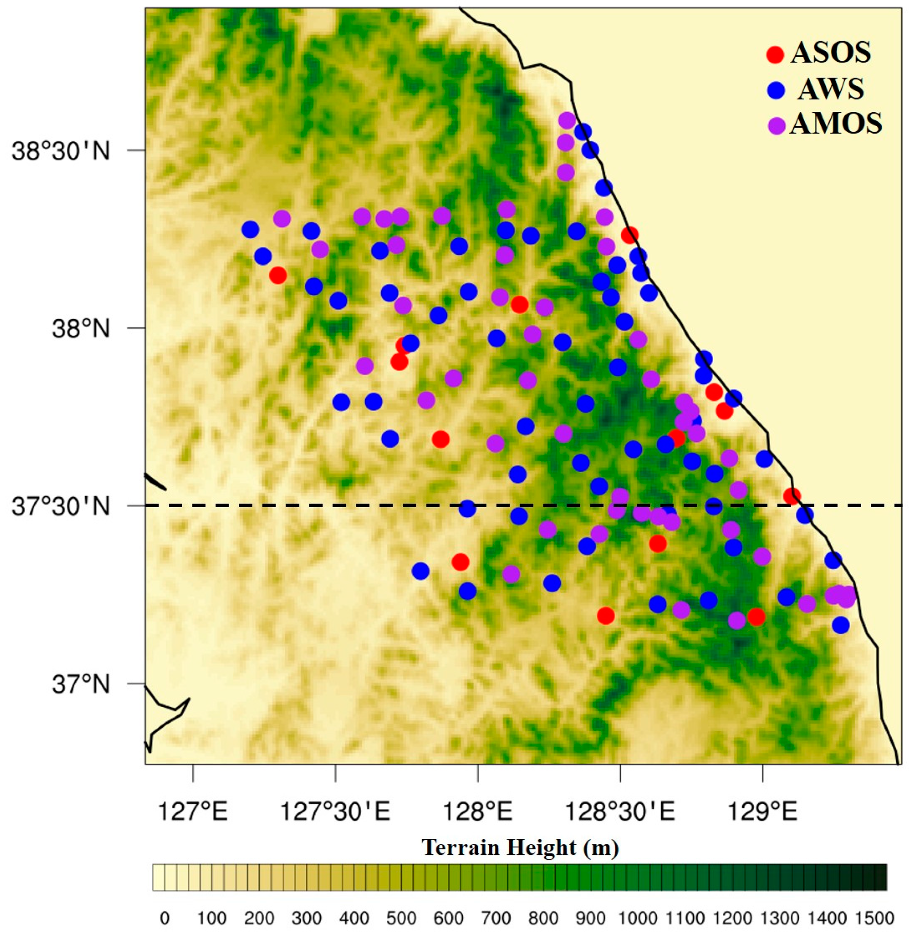
To validate the simulation results of each experiment, observational data from 122 stations in Gangwon-do were used. The Korea Meteorological Administration (KMA) has 14 Automated Synoptic Observing System (ASOS) stations, 59 Automated Weather Stations (AWSs), and the National Institute of Forest Science (NIFoS) has 49 Automatic Mountain Meteorology Observing System (AMOS) stations. Figure 3 shows the distribution of surface stations in d04. The meteorological factors used were temperature (°C) at 2 m, relative humidity (%) at 2 m, wind speed (m s−1) at 10 m, and accumulated precipitation (mm). The observed and simulated values were compared to the mean observation of all stations and simulations of all grids in which the station was located. TOP contrasts the 30-day period with CTL, whereas the SSE contrasts the average diurnal variation with CTL. Furthermore, the SSE results were examined by categorizing the observatories as eastern or western.
The RMSE and bias of each meteorological element were calculated and compared for the statistical analysis. The RMSE represents the average difference between the simulated and observed values. A positive value for bias indicates overestimation, whereas a negative value indicates underestimation. The RMSE and bias were computed as follows:
R M S E = 1 N i = 1 N ( M i O i ) 2
B i a s = 1 N i = 1 N M i O i
where N is the number of observations and simulations, O is the observed value, and M is the simulated value. The bias and RMSE were calculated as the averages of all stations and grids in which the stations were located, respectively.

3. Results

3.1. Subgrid-Scale Topographic Parameterization

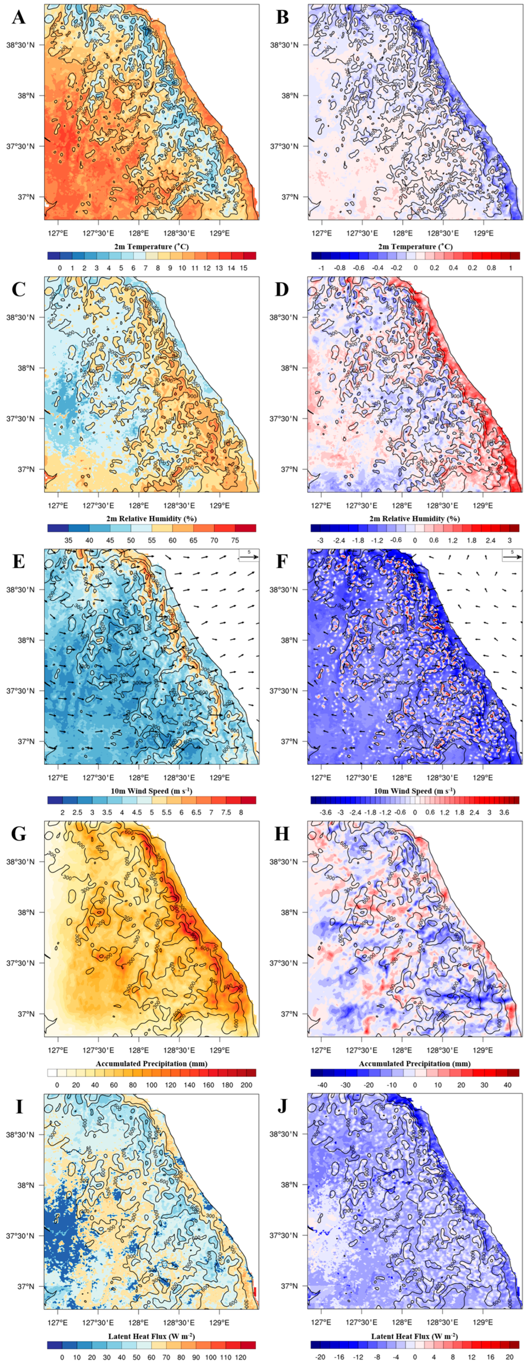
Figure 4 depicts the difference between the CTL and TOP experiments in terms of the monthly averaged horizontal distributions of simulated meteorological elements. The results of the 10 m wind speed simulation show a substantial difference between the two experiments. The simulated wind speed decreases over flat terrain and slopes and increases over hills and mountain tops (Figure 4F). The wind speed ranged from −3.63 to +3.44 m s−1, and a greater decline was simulated throughout the eastern Taebaek mountain range, where the slope is steeper than in other regions. When compared to the CTL experiment, the 2 m temperature in the TOP experiment showed a difference of between −0.77 °C and +0.19 °C, and the temperature tends to decrease towards the eastern coast and the mountain slope where the wind speed is lower (Figure 4B). Furthermore, the 2 m relative humidity increases when the 2 m temperature decreases, with a distribution ranging from −1.29% to +2.44% (Figure 4D). Monthly cumulative precipitation increased towards the east coast and decreased along the top of the high-altitude mountain area with a range of −35.68 to +28.60 mm (Figure 4H). This is caused by the decrease (increase) in latent heat flux from the surface (Figure 4J) along with 10 m wind speed decreases (increases). In the WRF model, temperature and humidity are influenced by sensible and latent heat flux emitted from the surface. Heat flux is proportional to aerodynamic conductance (AC), which measures how well the surface atmosphere mixes and the temperature and humidity difference between the surface and the atmosphere. AC is a function proportional to the wind; in the TOP experiment, when the surface wind speed was modified, AC decreased throughout the area where the wind speed decreased, and the heat flux reduced, resulting in a temperature drop and a rise in relative humidity in the lower atmosphere. Furthermore, there is a difference in the distribution of cumulative precipitation due to the change in water vapor levels, causing water vapor to converge in areas where the wind speed is low and diverge in areas where the wind speed is high. These results are similar to those of [27].
Figure 5 depicts the monthly averaged vertical distribution of the simulated meteorological elements from the CTL experiment and the contrast with the TOP experiment. The contour lines of meteorological components in mountainous regions are more complex than on flat land. As in the horizontal distribution, the vertical wind speed differential between the TOP and CTL experiments is notable (Figure 5F). The difference between the CTL experiment and the TOP experiment is −2.91 m s−1 to +0.34 m s−1, the wind speed near the surface and the slopes decreases, and the wind speed at the top of the mountain and at high altitude increases. The air temperature has a difference of −0.13 to +0.31 °C, and the temperature decreases in the Yeongdong region where the slope changes rapidly and increases in the Yeongseo region (Figure 5B). This was in good agreement with the results shown in the horizontal distribution. The water vapor mixing ratio increases when wind speed decreases but decreases where wind speed increases (Figure 5D). This is the outcome of water vapor convergence and divergence caused by changes in wind speed, as described above.
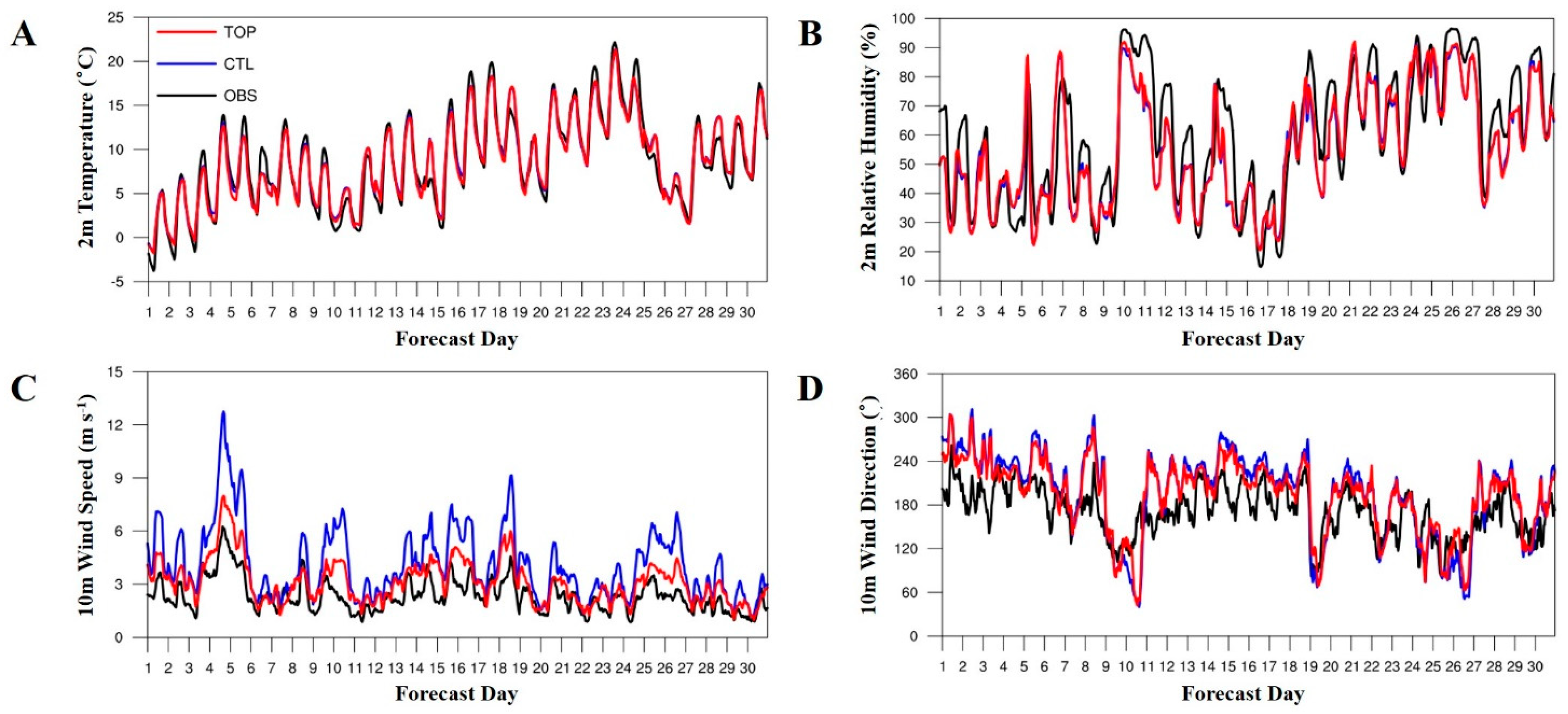
Figure 6 depicts the time series of the observed and simulated values. Table 3 shows the RMSE and bias between the averaged observations of surface stations and the averaged simulated values of grids where stations were located from the CTL and TOP experiments. When comparing the TOP experiment to the CTL experiment, the RMSE dropped by 53% from 2.18 m s−1 to 1.02 m s−1, and the bias decreased by 57% from 1.79 m s−1 to 0.77 m s−1. As a result, the wind speed, which had been overestimated, was greatly reduced in the TOP experiment (Figure 6C). There were also variations in other meteorological elements when the simulation results of the 10 m wind speed varied. At the 2 m temperature in the TOP experiment, the RMSE fell by 0.02 °C, and the bias decreased by 0.07 °C. Both the CTL and TOP experiments underestimated 2 m relative humidity; however, the RMSE and bias decreased by 0.26% and 0.17% in the TOP experiment, respectively. In both experiments, the cumulative precipitation was overestimated. The RMSE decreased by 2.02 mm, and the bias increased by 0.73 mm when compared with the CTL experiment. The simulation performance of the 10 m wind speed was substantially improved, while the other meteorological parameters showed minimal improvement.

3.2. Topographic Shading and Slope Parameterization

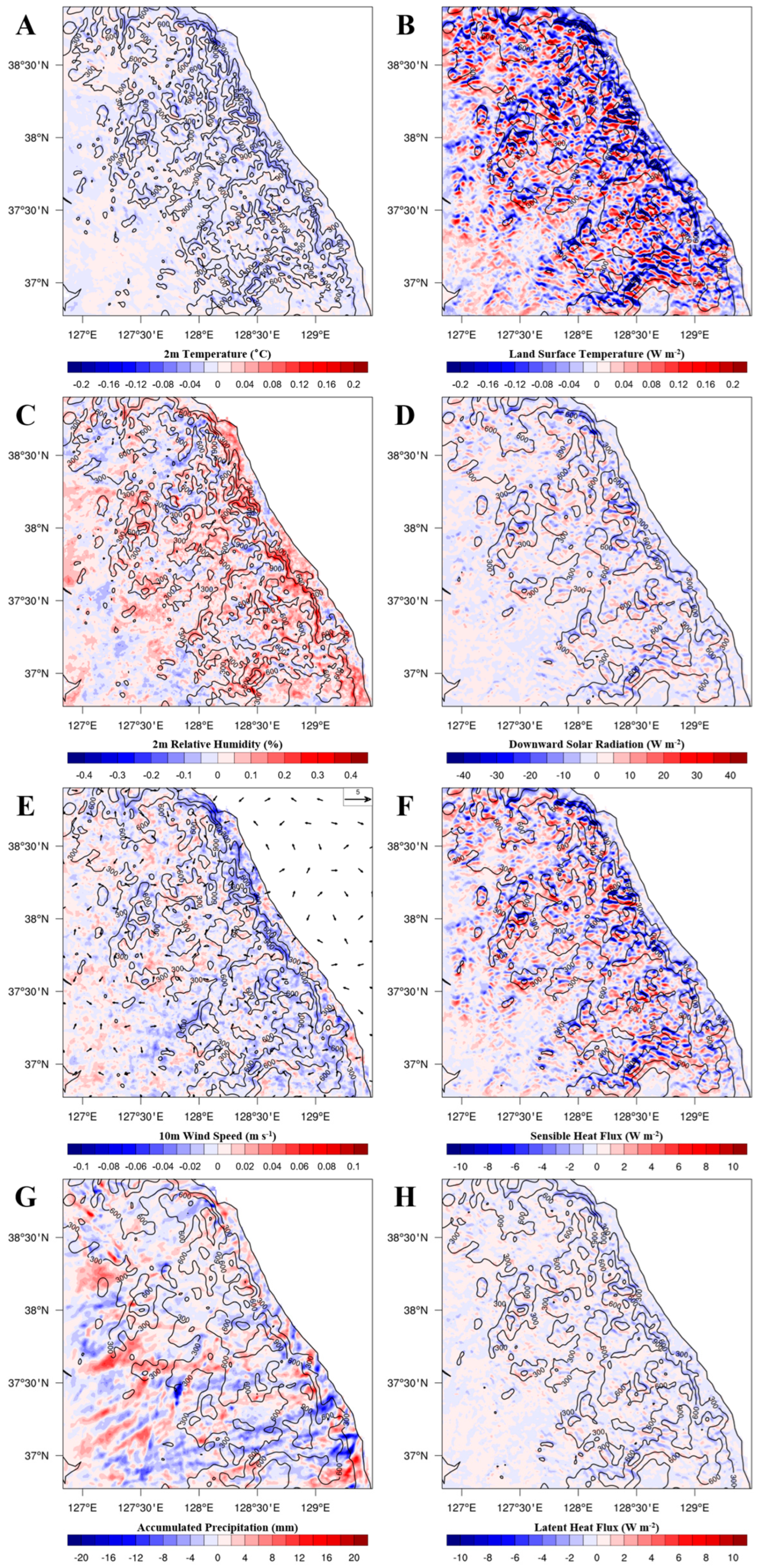
The monthly averaged horizontal difference distributions of meteorological components between the SSE and CTL experiments are depicted in Figure 7. In comparison with the CTL experiment, the 2 m relative humidity increased, and the 10 m wind speed decreased along the area where the 2 m temperature decreased in the SSE experiment. This was the result of correcting downward solar radiation by using slope and shading parameterizations; however, the values are rather close. When downward solar radiation increased (decreased) (Figure 7D), both the 2 m temperature and land surface temperatures increased (decreased) (Figure 7A,B), but the land surface temperature increased (decreased) more than the 2 m temperature, increasing (decreasing) the sensible and latent heat fluxes from the surface (Figure 7F,H). Other meteorological parameters were also affected by these changes. The distribution of increases and decreases was stronger along the mountain slope than along the plain, and the difference was noticeable in the southern and northern sides of the mountain. This is because the shading effect balanced out when the meteorological elements were averaged; and when the sun was in the east and west, it canceled each other; and when parameterizations are applied, the actual solar altitude reflects that tilted to the south.
Table 4 shows the RMSE and bias between the averaged observations and the simulated values from the CTL and SSE experiments. As shown in the horizontal distributions, there was no considerable difference in the simulated value. This is because the influence of the sun’s position was balanced out owing to the overall average; therefore, the effect of the parameterization was not clearly shown. To examine the parameterization effect in detail, we analyzed the time-averaged distributions for the horizontal 2 m temperature and the vertical atmospheric temperature of the SSE experiment. Furthermore, the surface stations were classified as eastern (45° ≤ A ≤ 135°) or western (225° ≤ A ≤ 315°), the diurnal cycle of the meteorological elements was examined, and the RMSE and bias were analyzed based on both real observations and simulated values.
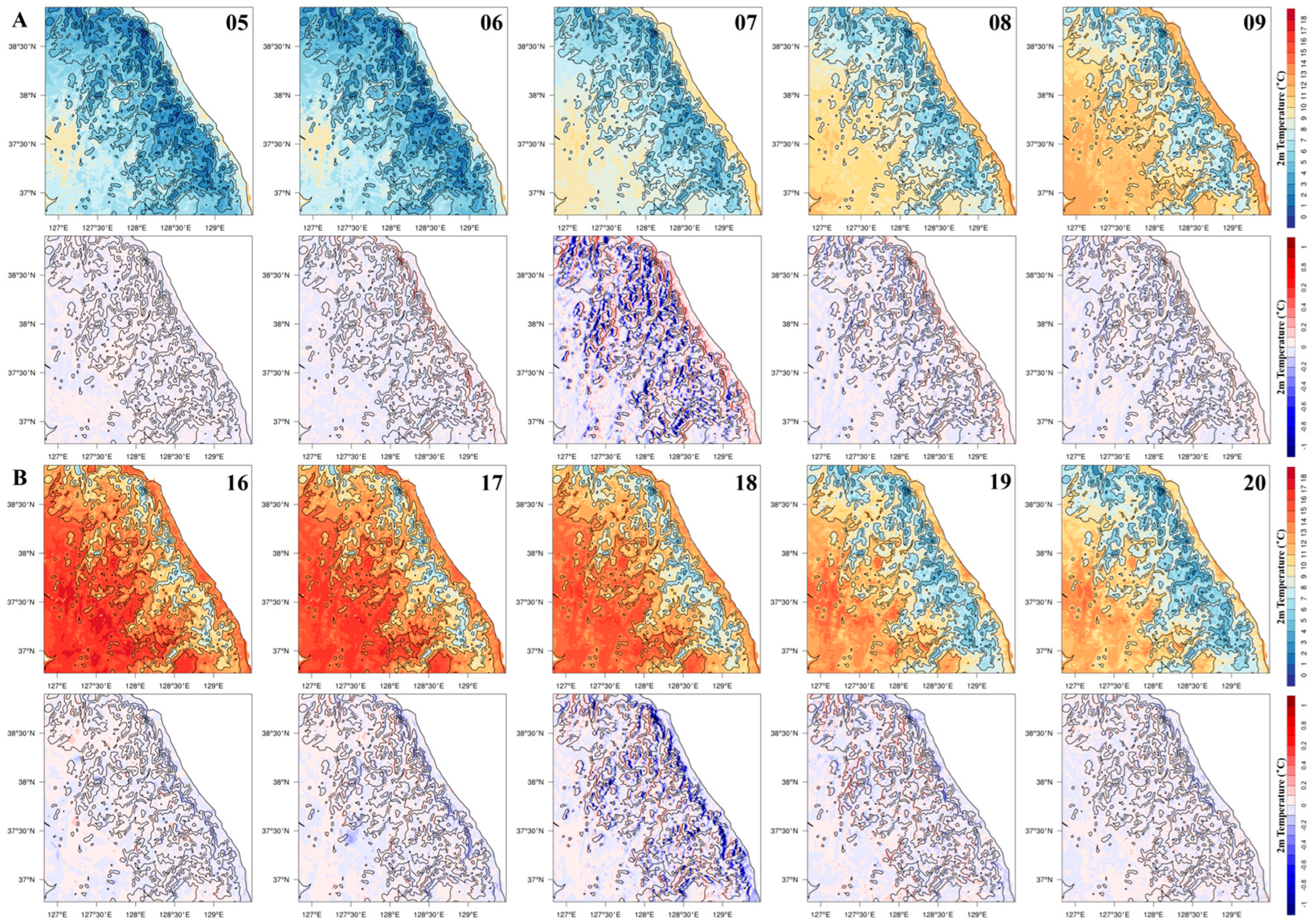
Figure 8 depicts the averaged horizontal distributions of sunrise (0500–0900 LST) and sunset time (1600–2000 LST) for 2 m temperature from the CTL experiment, and the difference with the SSE experiment. The contrast between the SSE CTL experiments was noticeable at sunrise (0700 LST) and sunset time (1800 LST). At sunrise, the temperature distribution ranged from −1.45 °C to +0.62 °C, with the temperature projected to be high on the eastern slope and low on the western slope (Figure 8A). At sunset, the temperature distribution ranged from −1.43 °C to +0.40 °C, and the temperature of the west slope increased while the temperature of the east side decreased, opposite to sunrise (Figure 8B). At other times, the difference was between −0.60 to +0.47 °C, and the east–west temperature differential due to the solar zenith angle remained.
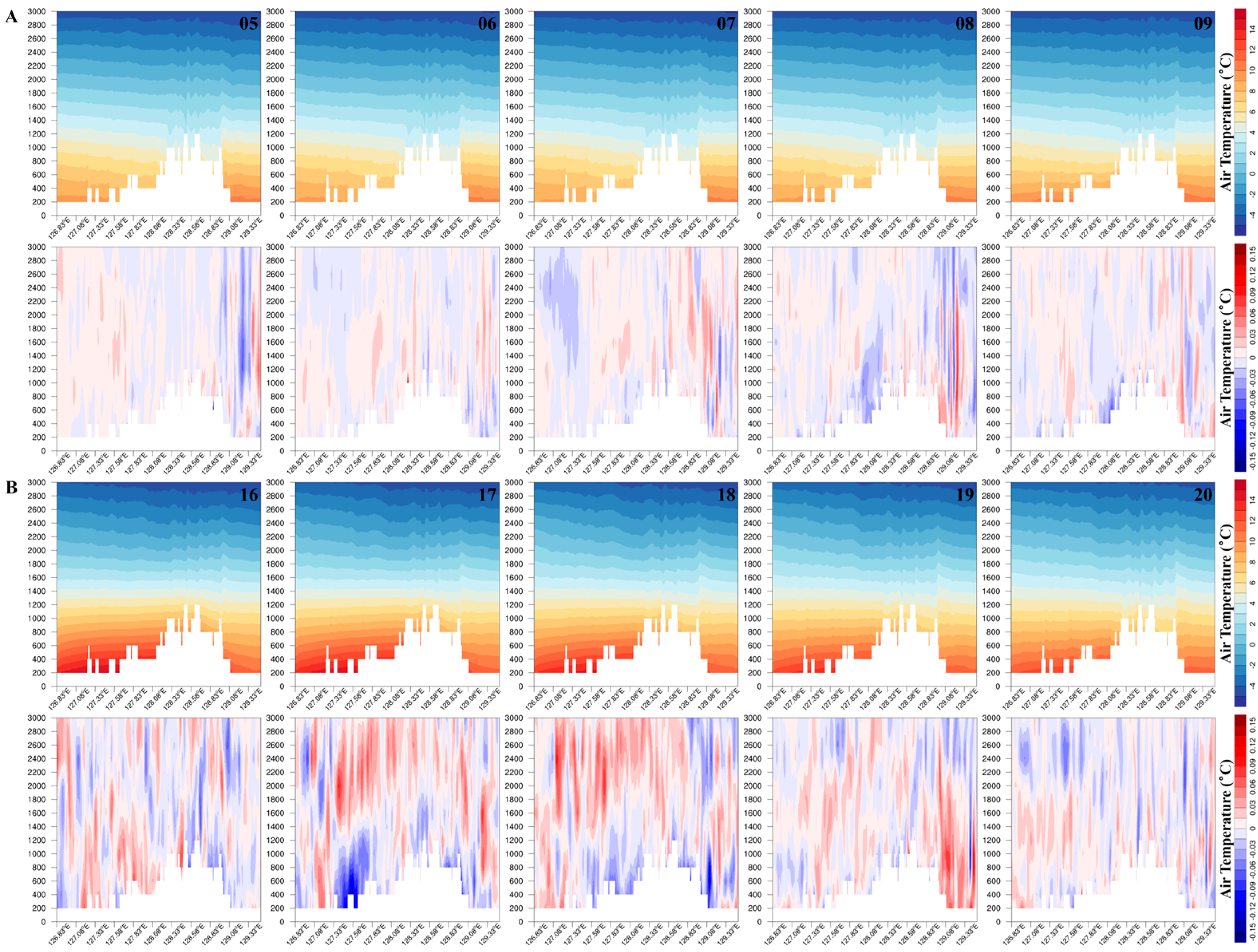
Figure 9 shows averaged vertical distributions of sunrise and sunset for atmospheric temperature from the CTL experiment compared with the SSE experiment. During sunrise, the temperature increased on the eastern slope of mountainous areas, and the temperature decreased on the western slope (Figure 9A). The range was −0.10 °C to 0.09 °C. During sunset, except for 1900 LST, the temperature of the eastern slope decreases. However, the temperature of the western slope increases just 1600 and 2000 LST (Figure 9B). The distribution of values ranges from −0.29 to +0.20 °C. In the vertical distribution of latitude 37.5°, the influence of the solar zenith angle was well reflected at sunrise, but conflicting results were found at sunset. This might be due to the fact that more precipitation was simulated at sunset than at sunrise and a different precipitation area was simulated compared to the CTL experiment.
The RMSE and bias between the averaged observations and simulated values of the diurnal cycle from the CTL and SSE experiments are shown in Table 5. As in the previous results, there was no quantitative improvement compared with the CTL experiment. In Figure 10, which shows the diurnal cycle of meteorological elements, differences are only found at sunrise and sunset times owing to slope and shading parameterizations. According to these results, the effect of parameterization is restricted to mountainous areas at specific times, sunrise and sunset, and the temperature was simulated more realistically than in the CTL experiment according to the solar zenith angle.

4. Concluding Remarks and Discussion

As the incidence and intensity of forest disasters have increased due to climate change [47], the accuracy of mountain weather simulation has become critical for mitigating the damage caused by forest disasters [48,49]. This study assessed the applicability of subgrid-scale topography, slope, and shading parameterizations over Gangwon-do to evaluate the performance of topographical effect parameterizations in the WRF model. Numerical simulations were conducted over a one-month period in April 2019, focusing on the Gangwon-do domain (d04) with a horizontal resolution of 1 km. The evaluation used simulation results from 0000 LST on 1 April 2019 to 2300 LST on 30 April 2019.
The subgrid-scale topographic parameterization simulated lower wind speeds over flat and sloped terrain and higher wind speeds in elevated areas, such as mountain tops and hills, by introducing a sink term that captures the terrain’s influence on the momentum equation. This parameterization significantly improved the simulation of 10 m wind speed, reducing the RMSE by 53% (from 2.18 to 1.02 m s−1) and the bias by 57% (from 1.79 to 0.77 m s−1), compared to the CTL experiment. These improvements are comparable to those reported in previous studies [23,24]. In areas where wind speeds decreased, 2 m temperature tended to decrease while 2 m relative humidity increased. Although the errors in temperature and humidity were reduced, the improvements were not as substantial as those observed for wind speed. Changes in surface wind also led to a redistribution of water vapor, with convergence in regions of reduced wind speed and divergence where wind speed increased. This dynamic altered the spatial distribution of the water vapor mixing ratio and impacted cumulative precipitation patterns.
The slope and shading parameterizations corrected the downward solar radiation by accounting for the influence of terrain slope and shadowing based on the solar zenith angle. These corrections captured the effects of slope heating and shadow-induced cooling, leading to corresponding increases or decreases in 2 m and ground temperatures in areas where downward solar radiation increased or decreased, respectively. Other meteorological variables were also affected by these adjustments. Specifically, the 2 m temperature increased on south-facing slopes and decreased on north-facing slopes, as the solar altitude was tilted southward throughout the analysis period. A time-averaged analysis of the 2 m temperature distribution showed an increase on east-facing slopes at sunrise and a decrease on west-facing slopes, with the opposite pattern observed at sunset. This diurnal trend was most prominent on mountain slopes and during sunrise and sunset hours (0700 and 1800 LST). Although there was no significant quantitative improvement in meteorological variables compared to the CTL experiment, the results were more physically realistic, as they reflected the influence of the solar zenith angle on surface energy balance and temperature distribution.
With improved surface wind speed simulation achieved through subgrid-scale topographic parameterization, and more realistic heat flow and temperature simulations enabled by slope and shading parameterizations, the accuracy of numerical weather simulations in mountainous regions can be significantly enhanced. These parameterizations should be fully considered for application in numerical simulations over complex terrain, particularly under fire weather conditions. Furthermore, additional improvements may be achieved by refining model resolution and selecting appropriate parameterization schemes tailored to the characteristics of the target region.
In this study, the performance and applicability of subgrid-scale topography, slope, and shading parameterizations, which have previously been insufficient for mountainous regions in Korea, were evaluated. The results are expected to serve as foundational data for future numerical simulation studies over complex mountainous terrains. In addition, these findings can provide insight to support forest fire risk forecasting where large-scale forest fires frequently occur in similar geographical regions around the world.
This study focused exclusively on the dry season, when the risk of forest fires is the highest in Korea. Consequently, the findings may not be fully applicable to other seasons, as Korea experiences four distinct seasonal climates. During the humid summer months, influenced by monsoon precipitation, wildfire risk is relatively low—only 9% of forest fires in the past 10 years have occurred in summer. Although fire risk is lower during this period, future research should investigate the influence of complex terrain under humid conditions, which may be particularly relevant for tropical regions characterized by higher moisture levels.
The parameterization employed in this study was based on a previous study conducted in northeastern Iberia, a region that may have different topographic characteristics from our study area. Therefore, future work should focus on developing a region-specific parameterization or calibrating the existing parameters to better suit the Korean landscape. Finally, it is worth noting that evaluating the improved meteorological outputs from the WRF model against actual wildfire events could further emphasize the model’s practical importance in fire management and prevention efforts.

Author Contributions

Y.J., S.K., Y.L. and J.H. planned the outline of the manuscript. Y.J., S.K. and Y.L. wrote the first draft of the manuscript. J.H. and J.L. designed the experiments. C.K. performed data analysis. K.J. contributed to data collection. All authors have read and agreed to the published version of the manuscript.

Funding

This research was supported by the National Institute of Forest Science under the project “Development of High-resolution Forest Micrometeorology Simulation Technology Considering Complex Mountainous Terrain Characteristics” (Grant No. FE0500-2019-01-2022), and by the Korea Meteorological Institute (Grant No. RS-2025-02221093).

Institutional Review Board Statement

Not applicable.

Informed Consent Statement

Not applicable.

Data Availability Statement

The original contributions presented in this study are included in the article. Further inquiries can be directed to the corresponding authors.

Conflicts of Interest

The authors declare no conflicts of interest, and the funders had no role in the design of the study; in the collection, analyses, or interpretation of data; in the writing of the manuscript; or in the decision to publish the results.

Abbreviations

The following abbreviations are used in this manuscript:
WRFWeather Research and Forecasting
RMSERoot Mean Square Error
NWPNumerical Weather Prediction

References

  1. KFS (Korea Forest Service). 2020 Forest Basic Statistics; Korea Forest Service: Daejeon, Republic of Korea, 2021; pp. 21–24. [Google Scholar]
  2. Kim, J.W.; Lee, J.G. A Qualitative Analysis of WRF Simulation Results of Typhoon ‘Rusa’ Case. Atmosphere 2007, 17, 393–405, (In Korean with English Abstract). [Google Scholar]
  3. Han, S.H.; Lee, J.G. A numerical simulation study on the sensitivity of WRF model in the wind field to the steepness of mountain slopes. Atmosphere 2007, 17, 349–364, (In Korean with English Abstract). [Google Scholar]
  4. Yun, H.S.; Um, M.J.; Cho, W.C.; Heo, J.H. Orographic precipitation analysis with regional frequency analysis and multiple linear regression. J. Korea Water Resour. Assoc. 2009, 42, 465–480. [Google Scholar] [CrossRef]
  5. Lee, J.H.; Jun, H.D. A methodology for rain gauge network evaluation considering the altitude of rain gauge. J. Wet. Res. 2014, 16, 113–124, (In Korean with English Abstract). [Google Scholar] [CrossRef]
  6. Yoon, S.; Jang, K.; Won, M. The spatial distribution characteristics of Automatic Weather Stations in the mountainous area over South Korea. Korean J. Agric. For. Meteorol. 2018, 20, 117–126. [Google Scholar]
  7. Vogt, J.V.; Viau, A.A.; Paquet, F. Mapping regional air temperature fields using satellite-derived surface skin temperatures. Int. J. Climatol. 1997, 17, 1559–1579. [Google Scholar] [CrossRef]
  8. Jang, K.; Kang, S.; Kimball, J.S.; Hong, S.Y. Retrieval of all-weather daily air temperature using MODIS and AMSRE data. Remote Sens. 2014, 6, 8387–8404. [Google Scholar] [CrossRef]
  9. Jang, K.; Won, M.; Yoon, S. Evaluation of the satellite-based air temperature for all sky conditions using the automated mountain meteorology station (AMOS) records: Gangwon Province case study. Korean J. Agric. For. Meteorol. 2017, 19, 19–26. [Google Scholar] [CrossRef]
  10. IPCC. Climate Change 2007: Synthesis Report; Core Writing Team, Pachauri, R.K., Reisinger, A., Eds.; Contribution of Working Groups 1, 2, and 3 to the Fourth Assessment Report of the Intergovernmental Panel on Climate Change; IPCC: Geneva, Switzerland, 2007. [Google Scholar]
  11. IPCC. Climate Change 2014: Synthesis Report; Core Writing Team, Pachauri, R.K., Meyer, L.A., Eds.; Contribution of Working Groups I, II, and III to the Fifth Assessment Report of the Intergovernmental Panel on Climate Change; IPCC: Geneva, Switzerland, 2014. [Google Scholar]
  12. IPCC. Climate Change 2021: The Physical Science Basis; Masson-Delmotte, V., Zhai, P., Pirani, A., Connors, S.L., Péan, C., Berger, S., Caud, N., Chen, Y., Goldfarb, L., Gomis, M.I., et al., Eds.; Contribution of Working Group I to the Sixth Assessment Report of the Intergovernmental Panel on Climate Change; IPCC, Cambridge University Press: Cambridge, UK; New York, NY, USA, 2021. [Google Scholar]
  13. Piñol, J.; Terradas, J.; Lloret, F. Climate warming, wildfire hazard, and wildfire occurrence in coastal eastern Spain. Clim. Change 1998, 11, 95–106. [Google Scholar]
  14. Flannigan, M.D.; Stocks, B.J.; Wotton, B.M. Climate change and forest fires. Sci. Total Environ. 2000, 262, 221–229. [Google Scholar] [CrossRef]
  15. Hély, C.; Flannigan, M.; Bergeron, Y.; McRae, D. Role of vegetation and weather on fire behavior in the Canadian mixedwood boreal forest using two fire behavior prediction systems. Can. J. For. Res. 2001, 31, 430–441. [Google Scholar] [CrossRef]
  16. Balshi, M.S.; McGUIRE, A.D.; Duffy, P.; Flannigan, M.; Walsh, J.; Melillo, J. Assessing the response of area burned to changing climate in western boreal North America using a Multivariate Adaptive Regression Splines (MARS) approach. Glob. Change Biol. 2009, 15, 578–600. [Google Scholar] [CrossRef]
  17. Lima, C.H.; AghaKouchak, A.; Randerson, J.T. Unraveling the role of temperature and rainfall on active fires in the Brazilian Amazon using a nonlinear Poisson model. J. Geophys. Res. Biogeosci. 2018, 123, 117–128. [Google Scholar] [CrossRef]
  18. Lu, W.; Zhong, S.; Charney, J.J.; Bian, X.; Liu, S. WRF simulation over complex terrain during a southern California wildfire event. J. Geophys. Res. Atmos. 2012, 117, D05125. [Google Scholar] [CrossRef]
  19. Goss, M.; Swain, D.L.; Abatzoglou, J.T.; Sarhadi, A.; Kolden, C.A.; Williams, A.P.; Diffenbaugh, N.S. Climate change is increasing the likelihood of extreme autumn wildfire conditions across California. Environ. Res. Lett. 2020, 15, 094016. [Google Scholar] [CrossRef]
  20. Dong, L.; Leung, L.R.; Qian, Y.; Zou, Y.; Song, F.; Chen, X. Meteorological environments associated with California wildfires and their potential roles in wildfire changes during 1984–2017. J. Geophys. Res. Atmos. 2021, 126, e2020JD033180. [Google Scholar] [CrossRef]
  21. Povak, N.A.; Hessburg, P.F.; Salter, R.B. Evidence for scale-dependent topographic controls on wildfire spread. Ecosphere 2018, 9, e02443. [Google Scholar] [CrossRef]
  22. Evers, C.; Holz, A.; Busby, S.; Nielsen-Pincus, M. Extreme Winds Alter Influence of Fuels and Topography on Megafire Burn Severity in Seasonal Temperate Rainforests under Record Fuel Aridity. Fire 2022, 5, 41. [Google Scholar] [CrossRef]
  23. Estes, B.L.; Knapp, E.E.; Skinner, C.N.; Miller, J.D.; Preisler, H.K. Factors influencing fire severity under moderate burning conditions in the Klamath Mountains, northern California, USA. Ecosphere 2017, 8, e01794. [Google Scholar] [CrossRef]
  24. Skamarock, W.C.; Klemp, J.B.; Dudhia, J.; Gill, D.O.; Barker, D.M.; Duda, M.G.; Huang, X.Y.; Wang, W.; Powers, J.G. NCAR TECHNICAL NOTE (NCAR/TN–475+ STR): A Description of the Advanced Research WRF Version 3; National Center for Atmospheric Research: Boulder, CO, USA, 2008. [Google Scholar]
  25. Mass, C.; Ovens, D. Fixing WRF’s high-speed wind bias: A new subgrid scale drag parameterization and the role of detailed verification. In Proceedings of the 24th Conference on Weather and Forecasting and 20th Conference on Numerical Weather Prediction, Preprints, 91st American Meteorological Society Annual Meeting, Seattle, WA, USA, 26 January 2011; Volume 23727, pp. 23–27. [Google Scholar]
  26. Jiménez, P.A.; Dudhia, J. Improving the representation of resolved and unresolved topographic effects on surface wind in the WRF model. J. Appl. Meteorol. Climatol. 2012, 51, 300–316. [Google Scholar] [CrossRef]
  27. Lee, J.; Shin, H.H.; Hong, S.Y.; Jimenez, P.A.; Dudhia, J.; Hong, J. Impacts of subgrid-scale orography parameterization on simulated surface layer wind and monsoonal precipitation in the high-resolution WRF model. J. Geophys. Res. Atmos. 2015, 120, 644–653. [Google Scholar] [CrossRef]
  28. Arthur, R.S.; Lundquist, K.A.; Mirocha, J.D.; Chow, F.K. Topographic Effects on Radiation in the WRF Model with the Immersed Boundary Method: Implementation, validation, and application to complex terrain. Mon. Weather Rev. 2018, 146, 3277–3292. [Google Scholar] [CrossRef]
  29. Lim, K.S.S.; Lim, J.M.; Shin, H.H.; Hong, J.; Ji, Y.Y.; Lee, W. Impacts of subgrid-scale orography parameterization on simulated atmospheric fields over Korea using a high-resolution atmospheric forecast model. Meteorol. Atmos. Phys. 2019, 131, 975–985. [Google Scholar] [CrossRef]
  30. Cheng, W.Y.Y.; Steenburgh, W.J. Evaluation of surface sensible weather forecasts by the WRF and the Eta models over the western United States. Weather Forecast. 2005, 20, 812–821. [Google Scholar] [CrossRef]
  31. Bernardet, L.; Nance, L.; Demirtas, M.; Koch, S.; Szoke, E.; Fowler, T.; Loughe, A.; Mahoney, J.L.; Chuang, H.; Pyle, M.; et al. The developmental testbed center and its winter forecast experiment. Bull. Amer. Meteor. Soc. 2008, 89, 611–627. [Google Scholar] [CrossRef]
  32. Seo, B.K.; Byon, J.Y.; Lim, Y.J.; Choi, B.C. Evaluation of surface wind forecast over the Gangwon province using the mesoscale WRF model. J. Korean Earth Sci. Soc. 2015, 36, 158–170. [Google Scholar] [CrossRef]
  33. Tsai, C.C.; Hong, J.S.; Chang, P.L.; Chen, Y.R.; Su, Y.J.; Li, C.H. Application of bias correction to improve WRF ensemble wind speed forecast. Atmosphere 2021, 12, 1688. [Google Scholar] [CrossRef]
  34. Mass, C.; Ovens, D. WRF model physics: Problems, solutions and a new paradigm for progress. In Proceedings of the 2010 WRF Users’ Workshop, Boulder, CO, USA, 15–21 June 2010. [Google Scholar]
  35. Papadopoulos, K.H.; Helmis, C.G. Evening and morning transition of katabatic flows. Bound.-Layer Meteorol. 1999, 92, 195–227. [Google Scholar] [CrossRef]
  36. Katurji, M.; Zawar-Reza, P.; Zhong, S. Surface layer response to topographic solar shading in Antarctica’s dry valleys. J. Geophys. Res. Atmos. 2013, 118, 12332–12344. [Google Scholar] [CrossRef]
  37. Lehner, M.; Whiteman, C.D.; Hoch, S.W.; Jensen, D.; Pardyjak, E.R.; Leo, L.S.; Di Sabatino, S.; Fernando, H.J.S.; Lehner, M.; Whiteman, C.D.; et al. A case study of the nocturnal boundary layer evolution on a slope at the foot of a desert mountain. J. Appl. Meteorol. Climatol. 2015, 54, 732–751. [Google Scholar] [CrossRef]
  38. Colette, A.; Chow, F.K.; Street, R.L. A numerical study of inversion-layer breakup and the effects of topographic shading in idealized valleys. J. Appl. Meteorol. 2003, 42, 1255–1272. [Google Scholar] [CrossRef]
  39. Garnier, B.J.; Ohmura, A.A. method for calculating direct shortwave radiation income of slopes. J. Appl. Meteorol. 1968, 7, 796–800. [Google Scholar] [CrossRef]
  40. Zängl, G. Formation of extreme cold-air pools in elevated sinkholes: An idealized numerical process study. Mon. Wea. Rev. 2005, 133, 925–941. [Google Scholar] [CrossRef]
  41. Hong, S.Y.; Lim, J.O.J. The WRF single-moment 6-class microphysics scheme (WSM6). J. Korean Meteorol. Soc. 2006, 42, 129–151. [Google Scholar]
  42. Iacono, M.J.; Delamere, J.S.; Mlawer, E.J.; Shephard, M.W.; Clough, S.A.; Collins, W.D. Radiative forcing by long-lived greenhouse gases: Calculations with the AER radiative transfer models. J. Geophys. Res. 2008, 113, D13103. [Google Scholar] [CrossRef]
  43. Hong, S.Y.; Noh, Y.; Dudhia, J. A new vertical diffusion package with an explicit treatment of entrainment processes. Mon. Weather Rev. 2006, 134, 2318–2341. [Google Scholar] [CrossRef]
  44. Jiménez, P.A.; Dudhia, J.; González-Rouco, J.F.; Navarro, J.; Montávez, J.P.; García-Bustamante, E. A revised scheme for the WRF surface layer formulation. Mon. Weather Rev. 2012, 140, 898–918. [Google Scholar] [CrossRef]
  45. Chen, F.; Dudhia, J. Coupling an advanced land surface-hydrology model with the Penn State–NCAR MM5 modeling system. Part I: Model implementation and sensitivity. Mon. Weather Rev. 2001, 129, 569–585. [Google Scholar] [CrossRef]
  46. Kain, J.S. The Kain–Fritsch convective parameterization: An update. J. Appl. Meteorol. 2004, 43, 170–181. [Google Scholar] [CrossRef]
  47. Mansoor, S.; Farooq, I.; Kachroo, M.M.; Mahmoud, A.E.D.; Fawzy, M.; Popescu, S.M.; Alyemeni, M.N.; Sonne, C.; Rinklebe, J.; Ahmad, P. Elevation in wildfire frequencies with respect to the climate change. J. Environ. Manag. 2022, 301, 113769. [Google Scholar] [CrossRef]
  48. Lim, C.H.; Kim, Y.S.; Won, M.; Kim, S.J.; Lee, W.K. Can satellite-based data substitute for surveyed data to predict the spatial probability of forest fire? A geostatistical approach to forest fire in the Republic of Korea. Geomat. Nat. Hazards Risk 2019, 10, 719–739. [Google Scholar] [CrossRef]
  49. Zhang, G.; Wang, M.; Liu, K. Forest fire susceptibility modeling using a convolutional neural network for Yunnan province of China. Int. J. Disaster Risk Sci. 2019, 10, 386–403. [Google Scholar] [CrossRef]
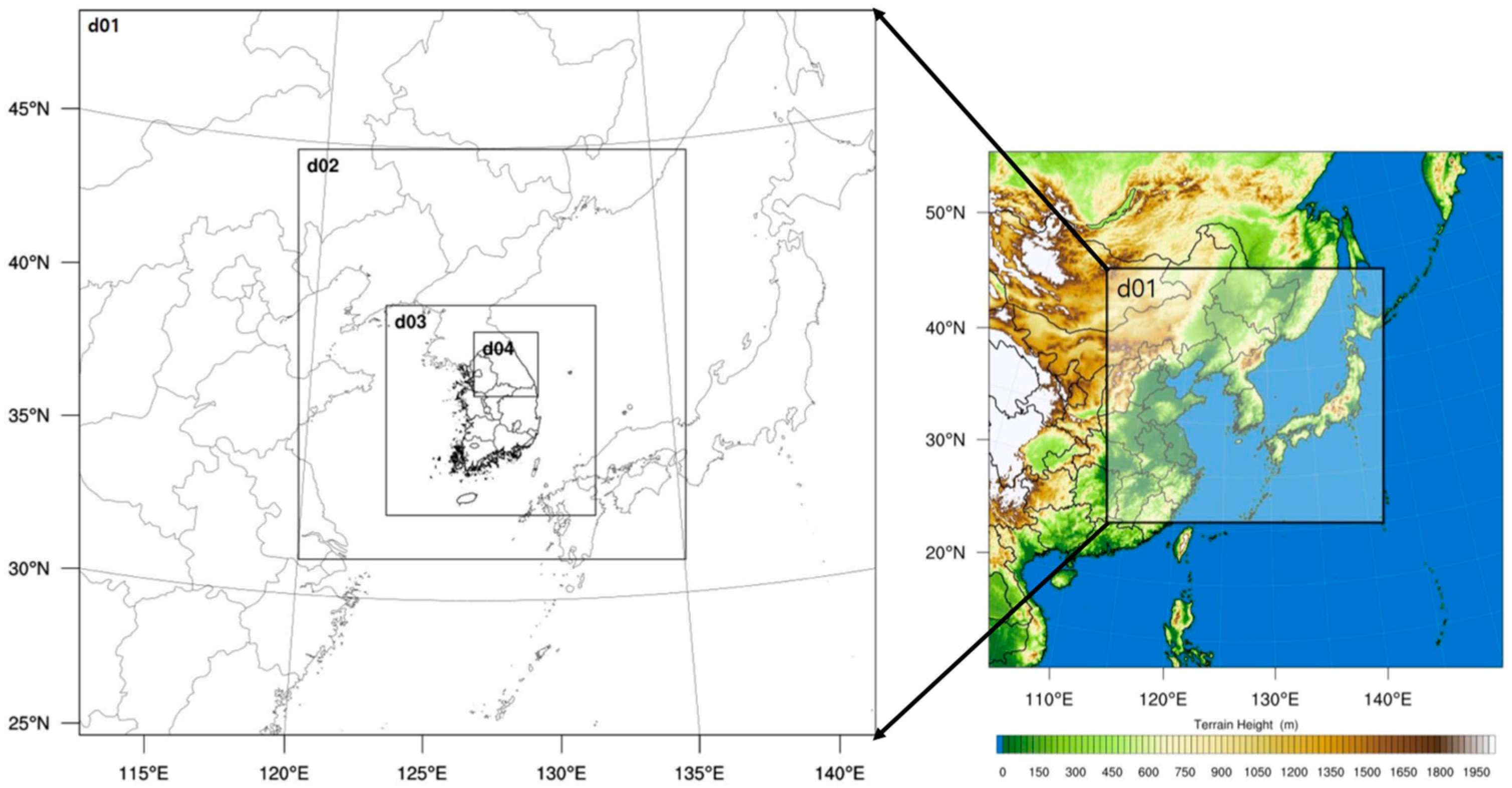
Figure 1. WRF domain configuration showing the range of four nested domains (Left) and simulation domain overlaid on the map (Right).
Fire 08 00196 g001
Figure 2. Terrain height (m) expressed in the model for each of the four nested domains.
Fire 08 00196 g002
Figure 3. Locations of the measurement stations in Gangwon-do. Dashed line represents the cross-section latitude (37.5° N).
Fire 08 00196 g003
Figure 4. Averaged horizontal distribution (CTL, left) and difference (TOP-CTL, right) of (A,B) 2 m temperature (°C), (C,D) 2 m relative humidity (%), (E,F) 10 m wind speed (m s−1) with wind vector, (G,H) accumulated precipitation (mm), and (I,J) surface latent heat flux (W m−2). The black line represents terrain height at 300 m intervals.
Fire 08 00196 g004
Figure 5. Averaged vertical distribution (CTL, left) and difference (TOP-CTL, right) of (A,B) air temperature (°C), (C,D) water vapor mixing ratio (g kg−1), (E,F) wind speed (m s−1), (G,H) zonal wind (m s−1), and (I,J) meridional wind (m s−1). The cross-sections have a latitude of 37.5° N.
Fire 08 00196 g005
Figure 6. Time series for the observed (black), CTL (blue), and TOP (red) observations of (A) 2 m temperature (°C), (B) 2 m relative humidity (%), (C) 10 m wind speed (m s−1), and (D) 10 m wind direction (°).
Fire 08 00196 g006
Figure 7. Averaged horizontal difference distribution (SSE-CTL) of (A) 2 m temperature (°C), (B) land surface temperature (°C), (C) 2 m relative humidity (%), (D) downward short wave flux (W m−2), (E) 10 m wind speed (m s−1) with wind vector, (F) sensible heat flux (W m−2), (G) accumulated precipitation (mm), and (H) latent heat flux (W m−2). The solid line represents terrain height expressed in the model at 300 m intervals.
Fire 08 00196 g007
Figure 8. Averaged 2 m temperature (°C) horizontal distribution of the CTL and averaged horizontal distribution difference (SSE-CTL). (A) 0500–0900 LST. (B) 1600–2000 LST.
Fire 08 00196 g008
Figure 9. Averaged air temperature (°C) vertical distribution of the CTL and averaged air temperature vertical distribution difference (SSE-CTL) (A) from 0500 to 0900 LST at hourly interval (B) from 1600 to 2000 LST at hourly interval.
Fire 08 00196 g009
Figure 10. Diurnal cycle of observed and simulated 2 m temperature (°C), 2 m relative humidity (%), and 10 m wind speed (m s−1). (A) Eastward station (45° ≤ A ≤ 135°) and (B) westward station (225° ≤ A ≤ 315°).
Fire 08 00196 g010
Table 1. WRF model configuration.
Versionv 3.7.1
Grib datasets6-h NCEP GDAS FNL
Simulation period31 March–1 May 2019
Domain
(126.9782° E,
37.5666° N)
d0127 km110 × 100
d029 km160 × 169
d033 km259 × 259
d041 km238 × 238
Vertical levels33
Model top pressure50 hPa
Nesting approachOne way
Model physics
MicrophysicsWRF Single-Moment 6-class
LW radiationRapid Radiative Transfer Model for GCMs
SW radiationRapid Radiative Transfer Model for GCMs
Surface layerRevised MM5 Monin–Obukhov
Land surfaceUnified Noah land surface model
PBLYonsei University
CumulusKain–Fritsch (new Eta) (only d01, d02)
Table 2. Overview of performed experiments.
Experiment
CTLControl run (default)
TOPApplying the subgrid-scale topographic parameterization
(topographic correction for surface winds)
SSEApplying the slope and shading parameterization
(neighboring-grid shadow effects and slope-dependent radiation)
Table 3. Statistics of the CTL and TOP for 2 m temperature (°C), 2 m relative humidity (%), 10 m wind speed (m s−1), and cumulative precipitation (mm).
OBSCTLTOP
AvgAvgRMSEBiasAvgRMSEBias
2 m T8.618.741.340.138.671.320.06
2 m RH60.4355.5611.86−4.8755.7311.60−4.70
10 m WS2.344.142.181.793.121.020.77
PRE62.2077.2228.6515.0276.4926.6314.29
Table 4. Statistics of the CTL and SSE for 2 m temperature (°C), 2 m relative humidity (%), 10 m wind speed (m s−1), and accumulated precipitation (mm).
OBSCTLSSE
AvgAvgRMSEBiasAvgRMSEBias
2 m T8.618.741.340.138.731.340.12
2 m RH60.4355.5611.86−4.8755.5911.89−4.84
10 m W2.344.142.181.794.132.181.79
PRE62.2077.2228.6515.0276.9228.4414.72
Table 5. Statistics of CTL and SSE with aspect direction for 2 m temperature (°C), 2 m relative humidity (%), and 10 m wind speed (m s−1).
OBSCTLSSE
AvgAvgRMSEBiasAvgRMSEBias
East2 m T9.199.330.590.149.320.610.13
2 m RH59.8854.267.01−5.6154.307.04−5.58
10 m W2.234.021.801.794.021.791.78
West2 m T8.228.220.810.008.220.79−0.01
2 m RH62.0356.627.72−5.4156.647.695.39
10 m W2.164.071.921.914.061.921.90
Disclaimer/Publisher’s Note: The statements, opinions and data contained in all publications are solely those of the individual author(s) and contributor(s) and not of MDPI and/or the editor(s). MDPI and/or the editor(s) disclaim responsibility for any injury to people or property resulting from any ideas, methods, instructions or products referred to in the content.